Ie2514631473

SahilGupta / International Journal of Engineering Research and Applications (IJERA) ISSN:
2248-9622 www.ijera.com Vol. 2, Issue 5, September- October 2012, pp.1463-1473
1463 | P a g e
Steady State Analysis of Self-Excited Induction Generator using
THREE Optimization Techniques
SahilGupta*
Student,Microelectronics
Bhai Maha Singh College of Engineering and Technology
ABSTARCT
It is well known that a three-phase
induction machine can be made to work as a self-
excited induction generator. In an isolated
application a three-phase induction generator
operates in the self-excited mode by connecting
three AC capacitors to the stator terminals. In a
grid connected induction generator the magnetic
field is produced by excitation current drawn
from the grid. In this dissertation the steady state
performance of an isolated induction generator
excited by three AC capacitor is analyzed with
the different optimization techniques. The effects
of various system parameters on the steady state
performance have been studied.
Keywords:- Artificial Neural Network, Induction
Generator, Genetic Algorithm
1.1 INTRODUCTION
An induction generator is a type of
electrical generator that is mechanically and
electrically similar to a poly-phase induction motor.
Induction generators produce electrical power when
their shaft is rotated faster than the synchronous
frequency of the equivalent induction motor.
Induction generators are often used in wind turbines
and some micro hydro installations due to their
ability to produce useful power at varying rotor
speeds.
Induction generators are not self-exciting,
meaning they require an external supply to produce
a rotating magnetic flux. The external supply can be
supplied from the electrical grid or from the
generator itself, once it starts producing power. The
rotating magnetic flux from the stator induces
currents in the rotor, which also produces a
magnetic field. If the rotor turns slower than the rate
of the rotating flux, the machine acts like an
induction motor. If the rotor is turned faster, it acts
like a generator, producing power at the
synchronous frequency. In induction generators the
magnetising flux is established by a capacitor bank
connected to the machine in case of stand alone
system and in case of grid connection it draws
magnetising current from the grid. It is mostly
suitable for wind generating stations as in this case
speed is always a variable factor.
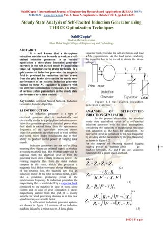
A self-excited induction generator systems
are shown in figure 1.1 consists of an induction
machine driven by a prime mover. A three-phase
capacitor bank provides for self-excitation and load
VARs requirements. As the load varies randomly
the capacitor has to be varied to obtain the desire
voltage.
Figure 1.1 Self-excited induction
generator systems
ANALYSIS OF SELF-EXCITED
INDUCTION GENERATOR
In the present dissertation, the standard
steady state equivalent circuit of a self-excited
induction generator with the usual assumptions,
considering the variation of magnetizing reactance
with saturation as the basis for calculation. The
equivalent circuit is nomalised to the base frequency
by dividing all the parameters by the p.u. frequency
as shown in figure 1.2.
For the purpose of obtaining required lagging
reactive power to maintain desired voltage at
machine terminals, XC and F are only unknown
parameters for a given speed and load.
Where
Z
Z
Z
ZS 3
2
1



(2)
 
F
X
F
R
R
X
Z
C
L
L
C
j
j


 2
1
(3)
X
F
R
Z S
S
j


2
(4)
 
  
X
X
F
j
R
X
F
j
R
jX
Z
R
M
R
R
R
M








 




3
(5)

1464 | P a g e
Since under steady state operation of SEIG IS can
not be equal to zero, therefore:
0

ZS
(6)
This equation after separation into real and
imaginary parts, can be rearranged into two
nonlinear equations which are solved using different
optimization techniques to obtain value of XC and F
after substituting XS= XR= XL.
    0
5
4
3
2
2
3
1
, 




 X
A
F
A
X
A
F
A
F
A
F
X
f C
C
C
(7)
      0
5
4
3
2
2
1
, 




 X
B
F
B
X
B
F
B
X
B
F
X
g C
C
C
C
(8)
Where the constants are defined as,
 
R
X
R
X
X
A L
L
L
M
L
2
1 2 





 A
A 1
2
  
R
R
R
X
X
A R
S
L
L
M




3
R
R
R
A R
L
S

4
   




 R
R
X
X
A S
L
L
M
5
X
X
X
B L
M
L
2
1 2 

  
X
X
R
R
R
B M
L
R
S
L



2



 B
B 1
3
  



 X
X
R
R
B L
M
L
S
4
 
R
R
R
B S
L
R



5
Objective function
2
2
2





 
 g
f
Z (9)
The relation between XM and Vg/F are given by:
K
V
K
X
F
g
M
2
1 








 (10)
Where K1 and K2 are depends on the design of the
machine.







 

Z
Z
Z
V
V T
g
1
2
1
(11)
Thus for a given value of RL and VT, the
value of Vg can be determined. With the known
values of Vg, F, XC, , RL and the generator’s
equivalent circuit parameters, the following
relations can be used for the computation of the
machine performance.
 
 
Z
Z
F
V
I
g
S
2
1

 (12)
 
 
 
jX
F
R
F
V
I
R
R
g
R





(13)
jX
F
R
I
jX
I
C
L
S
C
L



(14)
R
I
V L
L
T

(15)
 
X
F
V
VAR C
T
2

(16)
 




F
F
R
I
P
R
R
in
2
(17)
R
I
P L
L
out
2

(18)
To obtain the performance of self-excited
induction generator for the given value of
capacitance and speed, the unknown parameters are
the XM and F. The two non-linear equations after
substitution XS= XR= XL is given by:
     
    0
8
7
6
5
2
4
3
3
2
1
,









C
X
C
F
C
X
C
F
C
X
C
F
C
X
C
F
X
f
M
M
M
M
M
(19)
      0
5
4
3
2
2
1
, 




 D
F
D
D
D
F
D
X
D
F
X
g M
M
M
(20)
Where
R
X
C L
L
2
1


R
X
C L
L
2
2





 C
C 1
3



 C
C 2
4
 
R
R
R
X
C R
S
L
C



5
  R
R
R
R
R
R
X
X
C R
L
S
R
L
S
L
C




6
  



 R
R
X
C L
S
C
7
  



 R
R
X
X
C L
S
C
L
8
 
R
R
R
X
X
D R
S
L
C
L


 2
1

1465 | P a g e
  X
X
R
R
X
R
D C
L
R
S
L
L
2
2



  



 X
X
R
R
D L
C
L
S 2
3
  



 X
X
R
R
X
D L
C
L
S
L
2
4
 
R
R
R
X
D S
L
R
C



5
Objective function
2
2
2





 
 g
f
Z
(21)
By Finding these unknown parameters
using different optimization techniques and after
that performance of SEIG has been evaluated.
3.0 DIFFERENTOPTIMIZATION
TECHNIQUES FOR STEADY STATE
ANALYSIS OF SEIG GENETIC ALGORITHM
The genetic algorithm is a method for
solving optimization problems that is based on
natural selection, the process that drives biological
evolution. The genetic algorithm repeatedly
modifies a population of individual solutions. At
each step, the genetic algorithm selects individuals
at random from the current population to be parents
and uses them produce the children for the next
generation. Over successive generations, the
population evolves toward an optimal solution. The
GA has several advantages over other optimization
methods. It is robust, able to find global minimum
and does not require accurate initial estimates.
The genetic algorithm uses three main types of rules
at each step to create the next generation from the
current population:
Selection rules select the individuals, called parents
that contribute to the population at the next
generation.
Crossover rules combine two parents to form
children for the next generation.
Mutation rules apply random changes to individual
parents to form children.
3.2 PATTERN SEARCH
Pattern search is a subclass of direct search
algorithms, which involve the direct comparison of
objective function values and do not require the use
of explicit or approximate derivatives. Direct search
is a method for solving optimization problems that
does not require any information about the gradient
of the objective function. As opposed to more
traditional optimization methods that use
information about the gradient or higher derivative
to search for an optimal point, a direct search
algorithm searches a set of points around the current
point, looking for one where the value of the
objective function is lower than the value at the
current point. Direct search can be used to solve
problems for which the objective function is not
differential, or even continuous.
Pattern search over continuous variables is
defined via a finite set of directions used at each
search iteration. The direction set and a step length
parameter define a conceptual mesh centered about
the current iterate. Trial points are selected from the
mesh, evaluated, and compared to the current
iteration in order to select the next iterate. If an
improvement is found among the trial points, the
iteration is declared successful and the mesh is
retained; otherwise, the mesh is refined and a new
set of trial points is constructed. The key to
generating the mesh is the definition of the direction
set. This set must be sufficiently rich to ensure that
at least one of the directions is one of descent.
3.3 QUASI-NEWTON
Quasi-Newton methods, which are
currently the most robust and effective algorithms
for unconstrained optimization, are based on the
following set of ideas.
If Bk (definite matrix) is positive definite, the
direction –Bk-1 ∇f (xk) is always a descent direction
at xk, and we can perhaps get global convergence
(i.e. convergence starting anywhere) by searching in
those directions.
As long as Bk approximates the second
derivative matrix at least asymptotically, the method
is likely to work well locally (i.e. fast convergence).
For a quadratic function, a set of conjugate
directions, when searched sequentially, gives the
optimum solution in at most n iterations.
In terms of numerical computations for the inverse
of a matrix, the following formula is used for a low
rank update to a matrix
[A + uvT]-1 = A-1+(1/1+k) A-1 uvT A-1,
where k = vTA-1u Note that if A-1 is known, this is
much faster than computing [A + uvT]-1 directly.
This is a rank one update (uvT is a rank one matrix)
of the original matrix A. In particular, A + uuT is a
symmetric rank one update.
If Bk is updated by a small rank correction
to get Bk+1 then Bk+1-1 can be computed easily by
the above argument.
Quasi-Newton methods put all these ideas
together to construct approximations Bk to the
Hessian matrix at each stage. Note that some
updates work on Bk and update Bk and then find its
inverse, whereas some work directly on the inverse
of the second derivative approximation (Hk).
3.31 General Quasi-Newton Algorithm for
Minimizing a Function f
Start with x0 and H0 = I (approximation to the
inverse of the Hessian)
At step k,
dk = -Hk ∇f(xk)

1466 | P a g e
Find αk so as to (exactly or approximately)
minimize f(xk + αk dk)
xk+1 = xk + αk dk
Update Hk+1
Continue until a termination condition is satisfied.
EFFECTS OF VARIOUS SYSTEM
PARAMETERS BY PATTERN SEARCH
The performance characteristics of capacitor
excited, 3.7 KW, cage generator (detailed data given
in Appendix A) has been verified [4], [7] using
pattern search.
4.1Effects of Terminal Voltage on VAR
Requirements
The computed results for the given machine are
presented in figures 4.1 - 4.8. From these results, the
following salient features are observed.
Figure 4.1 shows the variations of frequency,
efficiency and stator current with output power at
constant terminal voltage and rated speed.
Figure 4.1
At constant terminal voltage the frequency
variation is negligible. The efficiency is good
throughout the power range and the stator current
increases with output power.
Figure 4.2 shows the variations of reactive power in
terms of reactive VAR and capacitance in terms of
susceptance with output power for various constant
terminal voltages and rated speed.
Figure 4.2
For constant terminal voltage, the
susceptance and VARs increases with output power.
With increase or decrease in the terminal voltage,
the VARs requirements increase or decrease
accordingly.
Figure 4.3 shows the variations of stator
and rotor currents with output power for various
constant terminal voltages and rated speed.
The magnitude of the rotor current is always less
than the stator current. This is because the rotor
current is approximately in quadrature with the
magnetizing current in both the motoring and
generating modes.
Figure 4.3
Figure 4.4 shows the variations of Cmin and
frequency with load resistance at constant terminal
voltage and rated speed.
0 0.1 0.2 0.3 0.4 0.5 0.6 0.7 0.8
0.4
0.5
0.6
0.7
0.8
0.9
1
Performancecharacteristics at Constant Terminal Voltage
Stator
Current,
Efficiency,
Frequency
(p.u.)
Output power(p.u.)
StatorCurrent
Efficiency
Frequency
VT= 1p.u.
0 0.2 0.4 0.6 0.8 1
0
0.5
1
1.5
Variation of Reactive VAR and Susceptance for different Terminal Voltages at rated Speed
Reactive
VAR
and
Susceptance
(p.u.)
Output power (p.u.)
VARS
Susceptance
VT= 1.2 p.u.
VT= 1 p.u.
VT= 0.8 p.u.
0 0.2 0.4 0.6 0.8 1
0
0.5
1
1.5
Variation of Stator and Rotor Current with Output Power
Stator
and
Rotor
Currents
(p.u.)
Output power (p.u.)
Stator Current
Rotor Current
VT= 0.8 p.u.
VT= 1 p.u.
VT= 1.2 p.u.

1467 | P a g e
Figure 4.4
As shown in figure the exciting capacitance
decreases as load resistance increases, whereas the
frequency increases.
Figure 4.5 and 4.6 shows the variations of
VARs with output power for different values of
stator and rotor resistance at constant terminal
Figure 4.5
Figure 4.6
It is seen from figures that a marginal reduction in
VAR requirement when stator and rotor resistance
are decrease.
Figure 4.7 shows the variation of VAR with output
power for different value of leakage reactance at
constant terminal voltage and rated sp
Figure 4.7
From figure the effect of leakage reactance on VAR
requirement at lower and higher loads are reverse,
the crossover taking place around the full load.
Figure 4.8 shows the variations of VAR with output
power for different values of K1 at constant voltage
and rated speed.
As shown in figure a small reduction in K1 there is
significant increase in VAR requirements.
Figure 4.8
4.1.1Effects of Capacitance on Terminal Voltage
presented in figures 4.9 - 4.16. From these results,
the following salient features are observed.
0 2 4 6 8 10 12 14 16 18 20
16
18
20
22
24
26
Variation of Cmin and Frequency with RL, at v = VT = 1 (p.u.)
Minimum
Capacitance
(micro
farad)
0 2 4 6 8 10 12 14 16 18 20
0.95
0.96
0.97
0.98
0.99
1
Frequency
(p.u.)
Load Resistance (p.u.)
Frequency (p.u.)
Minimum Capacitance (micro farad)
VT = 1 p.u.
Speed = 1 p.u.
0 0.1 0.2 0.3 0.4 0.5 0.6 0.7 0.8
0.45
0.5
0.55
0.6
0.65
0.7
0.75
Effect ofStator Resistance on VAR requirement
Reactive
VAR
(p.u.)
Output power (p.u.)
Rs* 0.8
Rs* 1
Rs* 1.2
VT= 1 p.u.
0 0.1 0.2 0.3 0.4 0.5 0.6 0.7 0.8
0.45
0.5
0.55
0.6
0.65
0.7
Effect ofRotor Resistance on VAR requirement
Reactive
VAR
(p.u.)
Output power (p.u.)
Rr* 0.8
Rr* 1
Rr* 1.2
VT= 1 p.u.
0 0.1 0.2 0.3 0.4 0.5 0.6 0.7 0.8
0.45
0.5
0.55
0.6
0.65
0.7
Effect of leakage Reactance on VAR requirement
Reactive
VAR
(p.u.)
Output power (p.u.)
XL* 0.8
XL* 1
XL* 1.2
VT = 1 p.u.
0 0.1 0.2 0.3 0.4 0.5 0.6 0.7 0.8
0.2
0.4
0.6
0.8
1
1.2
1.4
1.6
Effect ofMagnetising Reactance on VARrequirement
Reactive
VAR
(p.u.)
Output power (p.u.)
k1* 0.8
k1* 1
k1* 1.2
VT= 1 p.u.

1468 | P a g e
Figure 4.9 shows the variation of terminal voltage,
frequency and efficiency with output power at fixed
capacitance and constant speed.
Figure 4.9
It can be noted that the terminal voltage
and frequency decreases with output power, and
generator efficiency improves with load.
Figure 4.10 shows the variation of terminal voltage
and frequency with output power for different
values of capacitance and constant speed.
It can be seen that the terminal voltage are almost
parallel, indicating the proportional increase of VT
with capacitance. The frequency drop with output
power was not very much affected by the
capacitance.
Figure 4.10
Figure 4.11 and 4.12 shows the variations
of terminal voltage with output power for different
values of stator and rotor resistance at fixed
Figure 4.11
Figure 4.12
From figure it can be shown that at
increased value of stator and rotor resistance causes
more drooping the characteristics and decrease the
maximum output power.
Figure 4.13 shows the variation of terminal
voltage with output power for different values of
leakage reactance at fixed capacitance and constant
speed.
Figure 4.13
From figure it can be seen that for a given
value of capacitance and speed there is one value of
output power for which VT is independent of
leakage reactance. While lower value of
leaka
0 0.1 0.2 0.3 0.4 0.5 0.6 0.7 0.8
0.5
0.6
0.7
0.8
0.9
1
1.1
1.2
1.3
Performance Characteristics at given Capacitance and Speed
Terminal
Voltage,
Efficiency,
Frequency
(p.u.)
Output power(p.u.)
Terminal Voltage
Frequency
Efficiency
C= 25 micro farad
Speed = 1 p.u.
0 0.1 0.2 0.3 0.4 0.5 0.6 0.7 0.8 0.9 1
0.2
0.4
0.6
0.8
1
1.2
1.4
Variation of Terminal Voltage and Frequency with Output Power at different C
Terminal
voltage
and
Frequency
(p.u.)
Output power (p.u.)
Terminal Voltage
Frequency
C = 30 mf
C = 25 mf
C = 20 mf
0 0.1 0.2 0.3 0.4 0.5 0.6 0.7 0.8
0.6
0.7
0.8
0.9
1
1.1
1.2
1.3
1.4
Effect of Stator Resistance on Terminal voltage
Terminal
Voltage
(p.u.)
Output power (p.u.)
Rs* 0.8
Rs* 1
Rs* 1.2
C = 25 micro farad
Speed = 1 p.u.
0 0.1 0.2 0.3 0.4 0.5 0.6 0.7 0.8
0.6
0.7
0.8
0.9
1
1.1
1.2
1.3
1.4
Effect of Leakage Reactance on Terminal Voltage
Terminal
Voltage
(p.u.)
Output power (p.u.)
XL* 0.8
XL* 1
XL* 1.2
C = 25 micro farad
Speed = 1 p.u.
0 0.2 0.4 0.6 0.8 1 1.2 1.4
0.4
0.6
0.8
1
1.2
1.4
1.6
Effect of Magnetising Reactance on Terminal Voltage
Terminal
Voltage
(p.u.)
Output power (p.u.)
k1* 0.8
k1* 1
k1* 1.2
C = 25 micro farad
Speed = 1 p.u.

1469 | P a g e
ge reactance the terminal voltage improves.
with output power for different values of K1 at fixed
value of capacitance and constant speed.
Figure 4.14
From figure it can be seen that at increase value of
K1 causes increased terminal voltage and maximum
output
power. These changes are quite significant.
Figure 4.15 and 4.16 shows the variation of terminal
voltage and frequency with output power for
different values of speed at fixed capacitance.
Figure 4.15
Figure 4.16
From figure it can be seen that the terminal voltage
and frequency for the same output power increases
with speed. It is shown that both VT and frequency
are almost the same at all speed.
Effects of Various System Parameters by Genetic
Algorithm
The performance characteristics of capacitor
excited, 3.7 KW, cage generator (detailed data given
in Appendix A) has been verified [4], [7] using
genetic algorithm.
Effects of Terminal Voltage on VAR Requirements
presented in figures 4.17 - 4.24.
Figure 4.17 shows the variations of frequency,
efficiency and stator current with output power at
Figure 4.17
0 0.1 0.2 0.3 0.4 0.5 0.6 0.7 0.8
0.6
0.7
0.8
0.9
1
1.1
1.2
1.3
1.4
Effect ofRotorResistanceonTerminal Voltage
Terminal
Voltage
(p.u.)
Output power(p.u.)
Rr* 0.8
Rr* 1
Rr* 1.2
C= 25microfarad
Speed= 1p.u.
0 0.2 0.4 0.6 0.8 1 1.2 1.4 1.6
0.6
0.7
0.8
0.9
1
1.1
1.2
Effect ofSpeed on Frequency
Frequency
(p.u.)
Output power (p.u.)
v* 0.8
v* 1
v* 1.2
C= 25 micro farad
0 0.2 0.4 0.6 0.8 1 1.2 1.4 1.6
0.2
0.4
0.6
0.8
1
1.2
1.4
1.6
1.8
Effect ofSpeed on Terminal Voltage
Terminal
voltage
(p.u.)
Output power (p.u.)
v* 0.8
v* 1
v* 1.2
C = 25 micro farad
0 0.1 0.2 0.3 0.4 0.5 0.6 0.7 0.8
0.4
0.5
0.6
0.7
0.8
0.9
1
Performance characteristics at Constant Terminal Voltage
Stator
Current,
Efficiency
and
Frequency
(p.u.)
Output power (p.u.)
Stator Current
Efficiency
Frequency
VT = 1 p.u.

1470 | P a g e
Figure 4.19 shows the variations of stator and rotor
currents with output power for various constant
terminal voltages and rated speed.
Figure 4.19
Figure 4.20 shows the variations of Cmin and
frequency with load resistance at constant terminal
Figure 4.20
Figure 4.21 and 4.22 shows the variations of VARs
with output power for different values of stator and
rotor resistance at constant voltage and rated speed.
Figure 4.21
Figure 4.22
Figure 4.23 shows the variation of VAR with output
power for different values of leakage reactance at
Figure 4.23
0 0.2 0.4 0.6 0.8 1
0
0.5
1
1.5
VariationofStatorandRotorCurrent withOutput Power
Stator
and
Rotor
Currents
(p.u.)
Output power(p.u.)
StatorCurrent
RotorCurrent
VT= 0.8p.u.
VT= 1p.u.
VT= 1.2p.u.
0 2 4 6 8 10 12 14 16 18 20
16
18
20
22
24
26
Variation ofCmin and Frequency with RL, at v= VT= 1 (p.u.)
Minimum
Capacitance
(micro
farad)
0 2 4 6 8 10 12 14 16 18 20
0.95
0.96
0.97
0.98
0.99
1
Frequency
(p.u.)
Load Resistance (p.u.)
Frequency (p.u.)
Minimum Capacitance (micro farad)
VT= 1 p.u.
Speed = 1 p.u.
0 0.1 0.2 0.3 0.4 0.5 0.6 0.7 0.8
0.45
0.5
0.55
0.6
0.65
0.7
0.75
Effect of Stator Resistance on VAR requirement
Reactive
VAR
(p.u.)
Output power (p.u.)
Rs* 0.8
Rs* 1
Rs* 1.2
VT = 1 p.u.
0 0.1 0.2 0.3 0.4 0.5 0.6 0.7 0.8
0.45
0.5
0.55
0.6
0.65
0.7
0.75
Effect of Rotor Resistance on VAR requirement
Reactive
VAR
(p.u.)
Output power (p.u.)
Rr* 0.8
Rr* 1
Rr* 1.2
VT = 1 p.u.
0 0.1 0.2 0.3 0.4 0.5 0.6 0.7 0.8
0.45
0.5
0.55
0.6
0.65
0.7
Effect of leakage Reactance on VAR requirement
Reactive
VAR
(p.u.)
Output power (p.u.)
XL* 0.8
XL* 1
XL* 1.2
VT= 1 p.u.

1471 | P a g e
Figure 4.24 shows the variations of VAR with
output power for different values of K1 at constant
terminal voltage and rated speed.
Figure 4.24
Observations
There are close relation between the two results. The
genetic algorithm optimization technique gives
almost same results which we getting from the
pattern search optimization technique.
4.2.2 Effects of Capacitance on
Terminal Voltage
presented in figures 4.25 - 4.32.
In this case also the values which are obtained from
genetic algorithm optimization technique are much
closed with the values of the pattern search
optimization technique the figures are shown below.
Figure 4.25 shows the variation of terminal voltage,
frequency and efficiency with output power at fixed
Figure 4.25
and frequency with output power for different
values of capacitance and constant speed.
Figure 4.26
Figure 4.27 and 4.28 shows the variations of
terminal voltage with output power for different
values of stator and rotor resistance at fixed
Figure 4.27
0 0.1 0.2 0.3 0.4 0.5 0.6 0.7 0.8
0.2
0.4
0.6
0.8
1
1.2
1.4
1.6
Effect of Magnetising Reactance on VAR requirement
Reactive
VAR
(p.u.)
Output power (p.u.)
k1* 0.8
k1* 1
k1* 1.2
VT= 1 p.u.
0 0.1 0.2 0.3 0.4 0.5 0.6 0.7 0.8
0.5
0.6
0.7
0.8
0.9
1
1.1
1.2
1.3
Performance Characteristics at given Capacitance and Speed
Terminal
Voltage,
Efficiency
and
Frequency
(p.u.)
Output power (p.u.)
Terminal Voltage
Frequency
Efficiency
C = 25 micro farad
Speed = 1 p.u.
0 0.1 0.2 0.3 0.4 0.5 0.6 0.7 0.8 0.9 1
0.2
0.4
0.6
0.8
1
1.2
1.4
Variation of Terminal Voltage and Frequency with Output Power at different C
Terminal
voltage
and
Frequency
(p.u.)
Output power (p.u.)
Terminal Voltage
Frequency
C = 30 mf
C = 25 mf
C = 20 mf
0 0.1 0.2 0.3 0.4 0.5 0.6 0.7 0.8
0.6
0.7
0.8
0.9
1
1.1
1.2
1.3
1.4
Effect ofStatorResistanceonTerminal voltage
Terminal
Voltage
(p.u.)
Output power(p.u.)
Rs* 0.8
Rs* 1
Rs* 1.2
C= 25microfarad
Speed= 1p.u.

1472 | P a g e
Figure 4.28
with output power for different values of leakage
reactance at fixed capacitance and constant speed.
Figure 4.29
with output power for different values of K1 at fixed
value of capacitance and constant speed.
Figure 4.30
REFERENCES
[1] S.S. Murthy, O.P. Malik & A.K. Tandon,
“Analysis of self-excited induction
generators”, Proc. IEE, Vol. 129, Pt. C.,
No. 6, pp 260-265, Nov. 1982.
[2] S.S Murthy, B.P. Singh, C. Nagamani &
K.V.V. Satyanarayana, “Studies on the use
of conventional induction motor as self-
excited induction generators”, IEEE Trans.
EC, Vol. 3, No. 4, pp 842-848, Dec. 1988.
[3] A.K. Al Jabri & A.L. Alolah, “Capacitance
requirement for isolated self-excited
induction generator”, IEEE proceedings,
Vol. 137, Pt. B, No. 3, pp 154-159, May
1990.
[4] S.P. Singh, Bhim Singh & M.P. Jain,
“Performance characteristics and optimum
utilization of a cage machine as capacitor
excited induction generator”, IEEE Trans.
EC, Vol. 5, No. 4, pp 679-684, Dec. 1990.
[5] Bhim Singh, S.P. Singh & M.P. Jain,
“Design optimization of a capacitor self-
excited cage induction generator”, Electric
power system research, 22, pp 71-76, 1991.
[6] A.Wright, Genetic algorithms for real
parameters optimization, in J.E. Rawlines
(Ed.), Foundations of genetic algorithms
(San Mateo, CA: Morgan Kaufmann,
1991).
[7] L. Shridhar, Bhim Singh & C.S. Jha, “A
step towards improvements in the
characteristics of self excited induction
0 0.1 0.2 0.3 0.4 0.5 0.6 0.7 0.8
0.6
0.7
0.8
0.9
1
1.1
1.2
1.3
1.4
Effect ofRotorResistanceonTerminalVoltage
Terminal
Voltage
(p.u.)
Output power(p.u.)
Rr*0.8
Rr*1
Rr*1.2
C= 25microfarad
Speed= 1p.u.
0 0.1 0.2 0.3 0.4 0.5 0.6 0.7 0.8
0.6
0.7
0.8
0.9
1
1.1
1.2
1.3
1.4
EffectofLeakageReactanceonTerminalVoltage
Terminal
Voltage
(p.u.)
Outputpower(p.u.)
XL*0.8
XL*1
XL*1.2
C=25microfarad
Speed=1p.u.
0 0.2 0.4 0.6 0.8 1 1.2 1.4
0.4
0.6
0.8
1
1.2
1.4
1.6
Effect ofMagnetisingReactanceonTerminalVoltage
Terminal
Voltage
(p.u.)
Output power(p.u.)
k1*0.8
k1*1
k1*1.2
C= 25microfarad
Speed= 1p.u.

1473 | P a g e
generator”, IEEE Trans. EC, Vol. 8, No. 1,
pp 40-46, March 1993.
[8] J. Faiz, A.A. Dadgari, S. Horning & A.K.
Keyhani, “Design of a three-phase self-
excited induction generator”, IEEE Trans.
EC, Vol. 10, No. 3, pp 516-523, Sept.
1995.
[9] A.K. Sawhney, “A course in electrical
machine design”, 5th Edition, 1998,
Dhanpat rai & co. (Pvt.) Ltd.
[10] R. Bansal, T. Bhatti, & D. Kothari,
“Bibliography on the application of
induction generators in non-conventional
energy systems”, IEEE Trans. EC, 18(3),
pp 433-439, 2003.
[11] Y.N. Anagreh & I.S. Al-Kofahi, “Genetic
algorithm-based performance analysis of
self-excited induction generator”,
International Journal of Modeling and
Simulation, Vol. 26, No. 2, pp 175-179,
2006.
[12] M. Cunkas & R. Akkaya, “Design
optimization of induction motor by genetic
algorithm and comparison with existing
motor”, Mathematical and Computational
Applications, Vol. 11, No. 3, pp 193-206,
2006.
[13] Pattern Search Manual.
[14] Genetic Algorithm Manual.

Ie2514631473

Recommended

Recommended

More Related Content

What's hot

What's hot (19)

Viewers also liked

Viewers also liked (20)

Similar to Ie2514631473

Similar to Ie2514631473 (20)

Ie2514631473