1. Tutorial for Autodock and Autodock Tools
I. Establishing Access to the Programs
A. Autodock is in /usr/local/Autodock. The executables are autodock4
and autogrid4. Set up aliases in your .bashrc file:
alias autodock3=”/usr/local/Autodock/autodock4”
alias autogrid3=”/usr/local/Autodock/autogrid4”
B. Autodock tools are in /usr/local/MGLTools-1.5.4. Add to your .bashrc::
alias pmv=’/usr/local/MGLTools-1.5.4/bin/pmv’
alias adt=’/usr/local/MGLTools-1.5.4/bin/adt’
source /usr/local/MGLTools-1.5.4/bin/mglenv.sh
The aliases access the main parts of the tools; the last line sets up the
Python environment for the tools.
II. Preparing the Files
A. Two files in Protein DataBank (pdb) format are required for a docking
experiment: a structure for the protein and a structure for the ligand.
B. In general, the protein structure will be downloaded from the Protein
DataBank (www.rcsb.org), and the ligand structure will be created with
one of our modeling applications. You should inspect both files using less
or a text editor.
In the file from the PDB you want to identify any non-protein species that
will be removed later. This includes water (HOH) or other solvents,
sugars, and so on. Make a list of the types and their abbreviations.
Make sure you have a single copy of the protein in the file. Many
proteins crystallize as dimers or trimers, with each copy of the protein
containing a catalytic site. You must delete all extra chains. There are a
few proteins – the HIV protease is one – in which the catalytic site is
formed by the interaction of the chains. In this case, keep both chains.
In the ligand file, check the column that lists the residue or other structure
of which each atom is a part, and make sure that you have the three-letter
code for the amino acids (if the ligand is a peptide), or a code of your
choice for other ligands. PCModel puts UNK in this column when writing a
pdb file. Change this to a three-letter acronym for your ligand so that the
ligand can be selected properly for display in a program like JMol.

2. These files should be in the directory in which you choose to start.
C. If you are working with the tutorial from the AutoDock web site, “Using
AutoDock with AutoDock Tools”, the file as downloaded is both tarred and
gzipped (extensions .tar.gz). this means that multiple files have been
combined into one (tar) and compressed (gz). You must extract these by
typing in a shell window “tar –zxvf filename.tar.gz” (without the quotes, of
course). This will create your two pdb files and a subdirectory containing
the results from the docking for analysis.
III. Editing the Protein PDB File with AutoDock Tools (ADT)
We are going to fix any problems with the PDB files, such as missing bonds or
atoms, and remove extraneous structures such as water molecules. Before
beginning this section, inspect the PDB file to learn what such structures may be
present. We want to keep only the protein and such cofactors as may be bound
to it naturally.
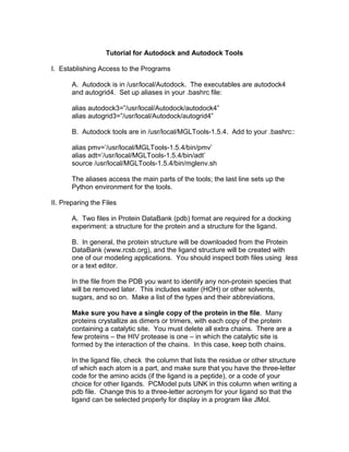
A. Start the ADT by typing ‘adt’ in a shell window in the directory where
you have placed your PDB files. Figure 1 showsthe ADT interface.
The ADT window has several parts:
(1) At the top are menus that access the functionality of PMV, the Python
molecular viewer, including reading and writing coordinates, creating
images, and modifying coordinates
(2) A row of buttons for quick access the PMV functions
(3) Menus to access AutoDock Tools functions.
(4) The molecule viewer window
(5) The Dashboard, for manipulating the molecule display.
B. Load the protein
From the File menu, choose Read Molecule, highlight the PDB file for your
protein, and click Open. Or, right click on PMV Molecules at the bottom of
the window and choose the protein pdb file.
For the tutorial, select hsg1.pdb
(1). As displayed, the protein appears white. You can color it according to
any of several schemes by selecting Color from the main menu bar, and

3. choosing any of the schemes listed there. In the widget that pops up, click
on All Geometries, and then on OK. You now have a pretty picture.
Alternatively, click on the diamond under “atom” on the dashboard to color
by atom type. (Figure 2)
Figure 1 The AutoDock Tools Window
C. Next, we remove the waters (those little red dots all over the display).
On the main menu bar, choose Select, Select From String. A widget pops
up (Figure 3):
In the Residue entry box, type HOH*. The asterisk is a “wild card”,
used in case the waters are numbered. It means accept any characters at

4. all following the H. Then type * in the Atom entry box; again the * is a wild
card, this time meaning “any atom”. Click select. If the PCOM level is not
already set to Atom (yellow button), you will get a message asking if
setting it there is OK. Click Yes. Then click Dismiss.
You should now see all of the waters marked with small yellow crosses
(Figure 4).
Figure 2. Protein hsg1 Loaded and Colored
On the main menu bar, choose Edit, Delete, Delete AtomSet. ADT will
ask if you really want to do this. Click Continue. The selected waters will
disappear.

5. Repeat this process for any other small molecules you need to get rid of
(check your pdb file!), such as other solvents like isopropyl alcohol (IPA),
N-acetylglucosamine (NAG), and other relics of the isolation and
crystallization procedures. Whole chains similarly can be deleted using
the Chain entry box.
Figure 3 The Select from String Widget
D. X-ray crystallography usually does not locate hydrogens; hence most
PDB files do not include them. But hydrogens, particularly those that can
hydrogen bond, are important in binding ligands.
(1) Choose Edit, Hydrogens, Add. Usually, you will choose Polar Only in
the widget that pops up, using Method noBondOrder, and renumbering
OK. This set of selections will add hydrogens to backbone N, and to
amine and hydroxyl side side chains. You will see them appear.
(2) Hide the protein by clicking the little gray box under “Show/Hide”.
If you wanted to interrupt processing at this point, you could choose File ->
Save -> Write PDB; however, we are going to add charges and AutoDock
atom types.
IV. Preparing the Ligand File with ADT
In this section information is added to the ligand pdb file to select bonds about
which segments of the ligand will be rotated. Charges are added, using the
Kollman scheme for peptide ligands and Gasteiger charges for other structures.

6. Before beginning, turn off display of the protein structure: click the Show/Hide
Molecule button, and then click the button next to the name of your protein. Click
the show/Hide button again to close the widget.
Figure 4 Water Molecules Selected for Deletion
A. Load the Ligand

7. (1) From the tan menubar just above the view window select: Ligand, Input
Molecule, Open Molecule. Click the file types button on the widget that appears
and select PDB files. Then choose the file containing your ligand, and click
Open. In the tutorial, this is ind.pdb
After a pause, a message will pop up, looking something like this (Figure 5)
Figure 5. Summary of Actions on Ligand:
ADT has done its job of assigning charges, making sure all hydrogens are
present, and detecting planar carbons in rings. TORSDOF is torsional degrees
of freedom.
B. Selecting Rotatable Segments
The initial step is selecting a set of atoms with respect to which other groups of
atoms will be rotated; this is called the Rigid Root. ADT tries to select a Root
with the minimum number of rotatable branches. A central benzene ring is a
popular choice.
(1) On the tan menubar, select Ligand -> Torsion Tree -> Detect Root. A small
green dot will appear, marking the choice.
(2) Next, select Ligand -> Torsion Tree -> Choose Torsions. The Torsion Count
widget appears (Figure 6).
The widget offers you several general selections of rotatable and non-rotatable
bonds.
(a) making peptide backbone bonds non-rotatable locks in the secondary
structure of the peptide; normally this is a poor choice

8. (b) At laboratory temperatures, the barrier to rotation around the CO-N bond of
an amide is too high to permit free rotation; if the ligand has amide functions,
click this button.
Figure 6. The Torsion Count Widget
Rotatable bonds also may be selected individually. If you do this, be careful!
Bonds within ring MUST be non-rotatable, and no more than 32 rotatable bonds
may be selected.
(3) It is possible, but optional, to select rotatable bonds that move the fewest
possible atoms, or the largest possible number. If you wish to do this, Select
Ligand -> Torsion Tree -> Set Number of Torsions (Figure 7).
Figure 7. Setting Number of Torsions in Ligand

9. You can see how this works by entering different numbers in the data window
and alternately clicking the fewest/most buttons while watching the molecule in
the display window.
When finished manipulating the torsions, click Done. The display now looks like
this (Figure 8):
Figure 8. Ligand with Torsions Selected
(4) To save the modified file, select Ligand -> Output -> Write PDBQT. Enter a
the name using the extension .pdbqt. (For the tutorial, this will be ind.pdbqt.)
The Q signifies that charges have been added, and the T that torsions have been
selected. Click Save. Then hide the root marker and ligand: click on its gray
Show/Hide marker.

10. V. Flexible Residues in the Protein
Beginning with AutoDock 4, support was added for making a portion of the
protein flexible, rather than treating it entirely as a rigid shape.
A. Redisplay hsg1 by clicking its gray Show/Hide marker.
Select Flexible Residues -> Input -> Choose Macromolecule. Then click on sg1
in the widget that appears and click on Select Molecule. You will get a message
that Gasteiger charges and AutoDock atom types have been added.
(1) If you are asked whether you want to merge the non-polar hydrogens, click
OK.
B. Select the residues to be flexible: Select -> Select from String.
(1) Click Clear Form to remove the waters. Working on the tutorial, type ARG8
in the Residue box, Click Add, and then Dismiss.
(2) At the bottom of the Dashboard, the Selected box should show “2 Residues”
(3) Now define the rotatable bonds in the selected residues: Flexible Residues -
> Choose Torsions in Currently Selected Residues. Everything except the
selected residues disappears, and the Torsion Count widget appears (Figure 9):
Figure 9. Torsion Count Widget for Flexible Residues in Protein
In the display, click on the bond between CA and CB in each residue to inactivate
it. (You may have to rotate the display in order to see both residues.) Six bonds
are now rotatable. Click Close. Clear the Selected box by clicking on the red
dots.

11. (4) Save the flexible residues: Flexible Residues -> Output -> Save Flexible
PDBQT. Type hsg1_flex.pdbqt in the File Browser window and Slick Save.
(5) Repeat, but save the Rigid PDBQT as hsg1_rigid.pdbqt.
C. Remove the original version of hsg1: Edit -> Delete -> Delete Molecule.
Choose hsg1, click on Delete Molecule, and click Dismiss.
VI. Further Preparation of the Protein Files
The next step is to prepare the grid files. Load the first protein file: Grid ->.
Macromolecule -> Open. Locate and click on hsg1_rigid.pdbqt.
A. ADT checks the charges. If it asks if you want to retain the existing charges,
click Yes. If you get a warning about non-integer charges, click OK. Dismiss any
other messages that may appear.
B. If your ligand file is still open, select the ligand: Grid -> Set Map Types ->
Choose Ligand. Select ind. If it is not open use: Grid -> Set Map types -> Open
Ligand, and choose ind.pdbqt. Both your protein and your ligand are now
displayed.
NOTE: The official tutorial at this point suggests that the AutoGpf Ligand widget
will open when you select the ligand. It does not. Before going on, use Grid ->
Set Map Types -> Directly to check that all atom types in your ligand are
represented. If not add the ones that are missing and close the widget.
(1) Open the Grid Options widget: Grid -> Grid Box.. It looks like this (Figure 10)
You will also notice that a blue and red box has appeared on the main display.
You can use the View menu on the Grid Options widget to control the display of
the blue box; for example, changing it to display as lines. If you rotate the
display, you can see that the box is 3-dimensional (Figure 11).
This is the box within which we are going to search; the Grid Box widget allows
you to set the size of the box, its location, and the number and spacing of the
points within it that will be tested.
(2) Use the thumbwheels to set the numbers of points to 60, 60, and 66. You
can do this by clicking and dragging on the wheel, or by right-clicking and
entering the number in the box that appears.
(3) This will center the grid box on the active site of the HIV-1 protease. These
numbers, of course, will vary from enzyme to enzyme. They are derived by
inspecting the pdb file and locating the coordinates of the active site residue(s).

12. (4) Use the File menu on the box to Close Saving Current. Then write the grid
point file: Grid -> Output -> Save GPF. Name the file “hsg1.gpf”.
C. You are now ready to run AutoGrid.
(1) Autogrid can be run from within AutoDock Tools. Choose Run -> AutoGrid
from the tan menu. The widget (Figure 12) appears.
Figure 10. The Grid Options Widget
Use the Browse button to navigate to /usr/local/AutoDock/autogrid4.
Parameter filename should be displayed automatically; Browse to it if it is not.
The log filename will be generated from the parameter filename, and the run
command in the last box will be displayed.

13. (2) Run the program by pressing Launch. A small process manager widget will
appear that will show you that AutoGrid is running, and allow you to terminate it if
desired.
AutoGrid will generate a series of Grid Parameter Map files, as seen in the
directory listing below (Figure 13).
Figure 11. The Grid Box
D. Next, we prepare the Docking Parameter file.

14. (1) From the tan menu, choose Docking -> Macromolecule -> Set Rigid
Filename, and select “hsg1_rigid.pdbqt”.
(2) Next, choose Docking -> Ligand -> Choose, and select “ind” A panel
appears (below) that allows you to set the initial position of the ligand and initial
values for the dihedrals. For the tutorial, simply click Accept.
(3) Set the Flexible Residues file: Docking -> Macromolecule -> Set Flexible
Residues Filename, and choose “hsg1_flex.pdbqt”. click Open.
Figure 12. The Run AutoGrid Widget
(3) To set the search parameters, choose Docking -> Search Parameters ->
Genetic Algorithm. Another widget appears (below). Select the Short setting,
which gives 250,000 energy evaluations. Click Accept.
Figure 13. Directory Listing Showing Maps Created by AutoGrid.

15. Figure 14. The dpf File Widget

16. (4) Choose the random number generator. Docking -> Docking Parameters.
Just go with the defaults in this tutorial. (Figure 15)
(5) Set the output filename and the choice of genetic algorithm. Docking ->
Output -> Lamarckian GA. Type in “ind.dlg” and click save.
E. Running AutoDock
AutoDock must be run in the directory where the macromolecule, ligand, gpf, dpf,
and map files are located.
In principle, AutoDock can be started from the Run menu in ADT just the way you
started AutoGrid. When I did this, AutoDock ran long enough to write the starting
conditions into the log file, and quit.
So then I opened a shell window, moving into the directory with the necessary
files, and typed at the command line:
autodock –p ind.dpf –l ind.glg &
And the program ran properly. When it finished, it printed the message:
“/usr/local/Autodock/autodock4 Successful Completion on “karplus”
If you used an alias other than “autodock” for the AutoDock executable,
replace “autodock” in the above command with whatever alias you used.

17. Figure 15. The Genetic Algorithm Widget
Figure 16. Choosing the Random Number Generator.