This document examines whether galaxy environments and the color-density relation can be robustly measured using photometric redshift (photo-z) surveys. It finds that:
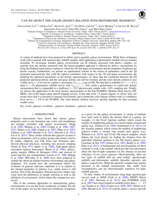
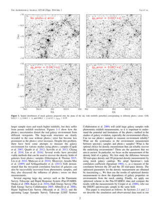
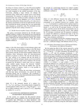
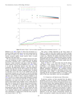
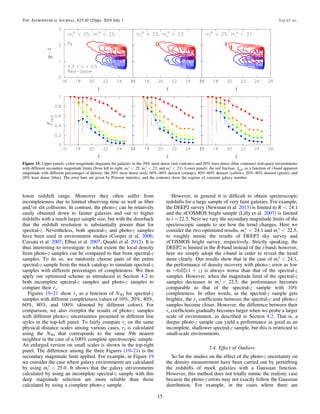
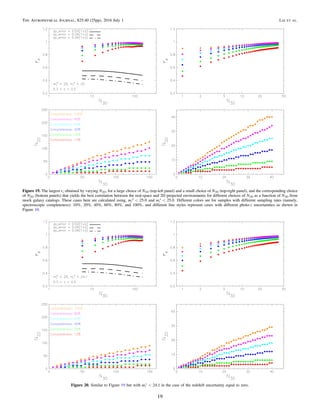
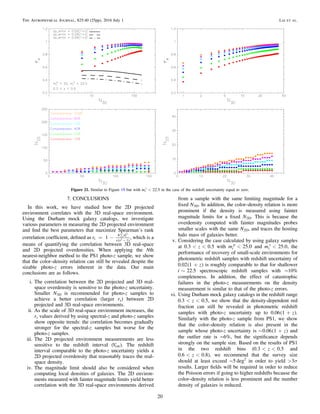
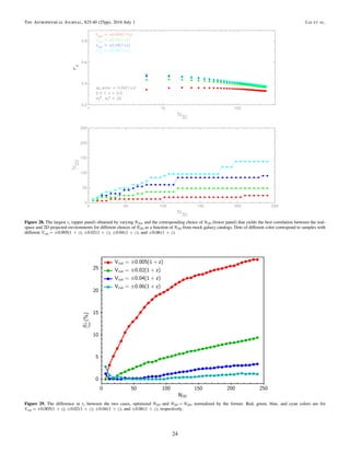
1) Using optimized parameters for density measurements, a correlation between 2D projected density measurements from photo-z surveys and true 3D density can still be revealed, even with photo-z uncertainties up to 0.06.
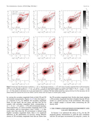
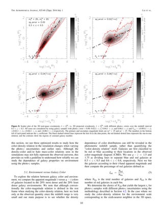
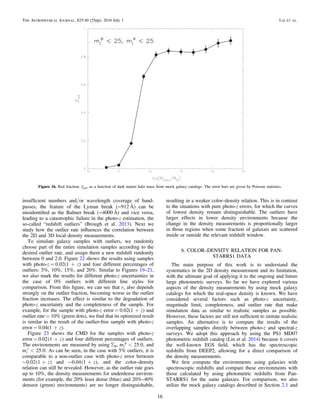
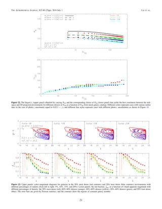
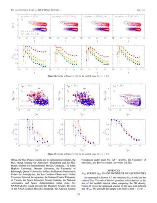
2) The color-density relation remains visible in photo-z surveys out to z=0.8, despite photo-z uncertainties of 0.02-0.06.
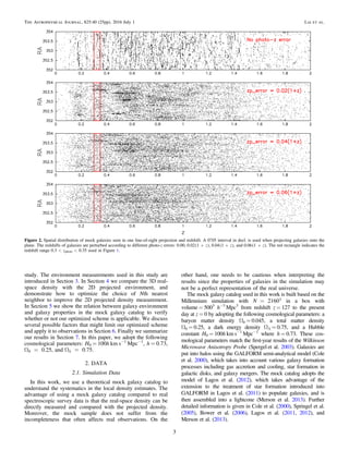
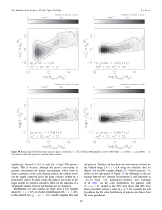
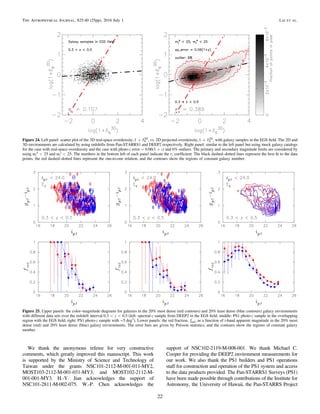
3) A deep (i=25 magnitude) photo-z survey with photo-z uncertainties of 0.02 can measure small-scale galaxy
The green valley_is_a_red_herring_galaxy_zoo_reveals_two_evolutionary_pathwaysSérgio Sacani
This document summarizes research using data from Galaxy Zoo, SDSS, and GALEX to study how star formation is quenched in low-redshift galaxies. The key findings are:
1) Taking galaxy morphology into account, the "green valley" is not a single transitional state, as was previously thought.
2) Only a small population of blue early-type galaxies rapidly transition across the green valley as their morphology transforms from disk to spheroid and star formation is quenched quickly.
3) The majority of blue star-forming galaxies have significant disks and retain their late-type morphology as their star formation rates decline very slowly.
4) Different evolutionary pathways are observed for early- and late-type
The yellow hypergiant HR 5171 A: Resolving a massive interacting binary in th...GOASA
HR 5171 A exhibits a complex appearance based on AMBER/VLTI observations. The observations reveal an unusually large star of approximately 1315 solar radii at a distance of 3.6 kiloparsecs. The source is surrounded by an extended nebula. The observations also show a high level of asymmetry in the brightness distribution, which is attributed to the discovery of a companion star located in front of the primary. Analysis of visual photometry data indicates the system has an orbital period of 1304 days, providing evidence it is a contact or over-contact eclipsing binary. Modeling suggests a total system mass of 39-79 solar masses and a high mass ratio of at least 10 for the companion. The discovery of the
The atacama cosmology_telescope_measuring_radio_galaxy_bias_through_cross_cor...Sérgio Sacani
A radiação cósmica de micro-ondas aponta para a matéria escura invisível, marcando o ponto onde jatos de material viajam a velocidades próximas da velocidade da luz, de acordo com uma equipe internacional de astrônomos. O principal autor do estudo, Rupert Allison da Universidade de Oxford apresentou os resultados no dia 6 de Julho de 2015 no National Astronomy Meeting em Venue Cymru, em Llandudno em Wales.
Atualmente, ninguém sabe ao certo do que a matéria escura é feita, mas ela é responsável por cerca de 26% do conteúdo de energia do universo, com galáxias massivas se formando em densas regiões de matéria escura. Embora invisível, a matéria escura se mostra através do efeito gravitacional – uma grande bolha de matéria escura puxa a matéria normal (como elétrons, prótons e nêutrons) através de sua própria gravidade, eventualmente se empacotando conjuntamente para criar as estrelas e galáxias inteiras.
Muitas das maiores dessas são galáxias ativas com buracos negros supermassivos em seus centros. Alguma parte do gás caindo diretamente na direção do buraco negro é ejetada como jatos de partículas e radiação. As observações feitas com rádio telescópios mostram que esses jatos as vezes se espalham por milhões de anos-luz desde a galáxia – mais distante até mesmo do que a extensão da própria galáxia.
Os cientistas esperam que os jatos possam viver em regiões onde existe um excesso de concentração da matéria escura, maior do que o da média. Mas como a matéria escura é invisível, testar essa ideia não é algo tão direto.
This document presents an analysis of transit spectroscopy observations of three exoplanets - WASP-12 b, WASP-17 b, and WASP-19 b - using the Wide Field Camera 3 instrument on the Hubble Space Telescope. The observations achieved almost photon-limited precision but uncertainties in the transit depths were increased by the uneven sampling of the light curves. The final transit spectra for all three planets are consistent with the presence of a water absorption feature at 1.4 microns, though the amplitude is smaller than expected from previous Spitzer observations possibly due to hazes. Due to degeneracies between models, the data cannot unambiguously constrain the atmospheric compositions without additional observations.
This document summarizes observations of the lensed galaxy HATLAS J142935.3-002836 (H1429-0028) from the Herschel-ATLAS survey. Optical spectroscopy revealed the foreground lens is at redshift 0.218, while the background galaxy is at redshift 1.027. High-resolution imaging from Hubble Space Telescope and Keck adaptive optics show the background galaxy is comprised of two components and a tidal tail, resembling a major merger. Analysis of ALMA observations of CO emission provides a dynamical mass estimate of one component as 5.8 ± 1.7 × 10¹⁰ M☉. Modeling of the spectral energy distribution indicates the total stellar mass is 1.32
Detection of lyman_alpha_emission_from_a_triply_imaged_z_6_85_galaxy_behind_m...Sérgio Sacani
We report the detection of Ly emission at 9538A
in the Keck/DEIMOS and HST WFC3
G102 grism data from a triply-imaged galaxy at z = 6:846 0:001 behind galaxy cluster MACS
J2129.4 0741. Combining the emission line wavelength with broadband photometry, line ratio upper
limits, and lens modeling, we rule out the scenario that this emission line is [O II] at z = 1:57. After
accounting for magnication, we calculate the weighted average of the intrinsic Ly luminosity to be
1:31042 erg s 1 and Ly equivalent width to be 7415A. Its intrinsic UV absolute magnitude at
1600A
is 18:60:2 mag and stellar mass (1:50:3)107 M, making it one of the faintest (intrinsic
LUV 0:14 L
UV) galaxies with Ly detection at z 7 to date. Its stellar mass is in the typical range
for the galaxies thought to dominate the reionization photon budget at z & 7; the inferred Ly escape
fraction is high (& 10%), which could be common for sub-L z & 7 galaxies with Ly emission. This
galaxy oers a glimpse of the galaxy population that is thought to drive reionization, and it shows
that gravitational lensing is an important avenue to probe the sub-L galaxy population.
This document describes observations of the galaxy ESO137-001 using the MUSE instrument on the VLT. The key points are:
1) MUSE observations reveal an extended gas tail stretching over 30 kpc from the galaxy, tracing ongoing ram pressure stripping as it falls into the Norma galaxy cluster.
2) Analysis of the gas kinematics and stellar velocity field show that ram pressure has removed the interstellar medium from the outer disk while the primary tail is still fed by gas from the galaxy center.
3) The stripped gas retains evidence of the disk's rotational velocity out to 20 kpc downstream, indicating the galaxy is moving radially through the cluster. Beyond this the gas shows greater turbulence,
“A ring system detected around the Centaur (10199) Chariklo”GOASA
- The Centaur object (10199) Chariklo was observed to occult a star, revealing the presence of two narrow rings around the object.
- The rings have widths of about 7 km and 3 km, and orbital radii of 391 km and 405 km from the center of Chariklo.
- Evidence supports the rings being composed of water ice and their geometry explaining the dimming and changing spectrum of Chariklo observed between 1997 and 2008. The discovery of rings around a minor planet is a first for the Solar System.
Todo mundo sabe que os raios produzidos pela Estrela da Morte em Guerra nas Estrelas não pode existir na vida real, porém no universo existem fenômenos que as vezes conseguem superar até a mais surpreendente ficção.
A galáxia Pictor A, é um desses objetos que possuem fenômenos tão espetaculares quanto aqueles exibidos no cinema. Essa galáxia localiza-se a cerca de 500 milhões de anos-luz da Terra e possui um buraco negro supermassivo no seu centro. Uma grande quantidade de energia gravitacional é lançada, à medida que o material cai em direção ao horizonte de eventos, o ponto sem volta ao redor do buraco negro. Essa energia produz um enorme jato de partículas que viajam a uma velocidade próxima da velocidade da luz no espaço intergaláctico, chamado de jato relativístico.
Para obter imagens desse jato, os cientistas usaram o Observatório de Raios-X Chandra, da NASA várias vezes durante 15 anos. Os dados do Chandra, apresentados em azul nas imagens, foram combinados com os dados obtidos em ondas de rádio a partir do Australia Telescope Compact Array, e são aparesentados em vermelho nas imagens.
The document summarizes the results of a statistical analysis comparing the characteristics of galaxies with and without detected water megamaser emission. The analysis finds that maser galaxies tend to have higher levels of reddening and extinction, are more massive and luminous, and harbor more massive black holes. However, galaxies with very massive black holes do not host masers. The analysis identifies parameter ranges that are associated with higher detection rates of maser emission, including narrow ranges of electron density, black hole mass, and Eddington ratio. Principal component analysis and discriminant analysis indicate quantifiable differences between maser and non-maser galaxies that can be used to target future surveys and potentially increase detection rates.
This document summarizes observations of the Andromeda satellite dwarf galaxy Cassiopeia III using the WIYN pODI imager. Preliminary analysis of the color-magnitude diagram shows stars that coincide with a 12-Gyr isochrone at the known metallicity and distance of Cas III. Structural parameters were measured including position angle, ellipticity, and half-light radius that are consistent with previous work but have smaller uncertainties. Future work will include PSF photometry, deriving the surface brightness profile and distance, and analyzing the metallicity distribution.
First identification of_direct_collapse_black_holes_candidates_in_the_early_u...Sérgio Sacani
The first black hole seeds, formed when the Universe was younger than ⇠ 500Myr, are recognized
to play an important role for the growth of early (z ⇠ 7) super-massive black holes.
While progresses have been made in understanding their formation and growth, their observational
signatures remain largely unexplored. As a result, no detection of such sources has been
confirmed so far. Supported by numerical simulations, we present a novel photometric method
to identify black hole seed candidates in deep multi-wavelength surveys.We predict that these
highly-obscured sources are characterized by a steep spectrum in the infrared (1.6−4.5μm),
i.e. by very red colors. The method selects the only 2 objects with a robust X-ray detection
found in the CANDELS/GOODS-S survey with a photometric redshift z & 6. Fitting their
infrared spectra only with a stellar component would require unrealistic star formation rates
(& 2000M# yr−1). To date, the selected objects represent the most promising black hole seed
candidates, possibly formed via the direct collapse black hole scenario, with predicted mass
> 105M#. While this result is based on the best photometric observations of high-z sources
available to date, additional progress is expected from spectroscopic and deeper X-ray data.
Upcoming observatories, like the JWST, will greatly expand the scope of this work.
Detection of solar_like_oscillations_in_relies_of_the_milk_way_asteroseismolo...Sérgio Sacani
Asteroseismic constraints on K giants make it possible to infer radii, masses and ages of tens
of thousands of field stars. Tests against independent estimates of these properties are however
scarce, especially in the metal-poor regime. Here, we report the detection of solar-like
oscillations in 8 stars belonging to the red-giant branch and red-horizontal branch of the globular
cluster M4. The detections were made in photometric observations from the K2 Mission
during its Campaign 2. Making use of independent constraints on the distance, we estimate
masses of the 8 stars by utilising different combinations of seismic and non-seismic inputs.
When introducing a correction to the Δν scaling relation as suggested by stellar models, for
RGB stars we find excellent agreement with the expected masses from isochrone fitting, and
with a distance modulus derived using independent methods. The offset with respect to independent
masses is lower, or comparable with, the uncertainties on the average RGB mass
(4 − 10%, depending on the combination of constraints used). Our results lend confidence to
asteroseismic masses in the metal poor regime. We note that a larger sample will be needed
to allow more stringent tests to be made of systematic uncertainties in all the observables
(both seismic and non-seismic), and to explore the properties of RHB stars, and of different
populations in the cluster.
This document discusses a study that used difference imaging techniques to search for variable stars and microlensing events in the elliptical galaxy Centaurus A. The study obtained deep photometric data over almost two months using the Wide Field Imager on the ESO/MPG 2.2 m telescope. It detected 271 variable stars in Centaurus A with a detection limit of magnitude 24.5. Based on a simple model of Centaurus A's halo, the study estimated it could detect around 4 microlensing events per year, but a higher sensitivity is needed for a meaningful microlensing survey. The spatial distribution of any microlensing events could help constrain the shape of Centaurus A's dark matter halo.
Discovery of rotational modulations in the planetary mass companion 2m1207b i...Sérgio Sacani
Rotational modulations of brown dwarfs have recently provided powerful constraints on the properties
of ultra-cool atmospheres, including longitudinal and vertical cloud structures and cloud evolution.
Furthermore, periodic light curves directly probe the rotational periods of ultra-cool objects. We
present here, for the first time, time-resolved high-precision photometric measurements of a planetarymass
companion, 2M1207b. We observed the binary system with HST/WFC3 in two bands and with
two spacecraft roll angles. Using point spread function-based photometry, we reach a nearly photonnoise
limited accuracy for both the primary and the secondary. While the primary is consistent with
a flat light curve, the secondary shows modulations that are clearly detected in the combined light
curve as well as in di↵erent subsets of the data. The amplitudes are 1.36% in the F125W and 0.78%
in the F160W filters, respectively. By fitting sine waves to the light curves, we find a consistent period
of 10.7+1.2
−0.6 hours and similar phases in both bands. The J- and H-band amplitude ratio of 2M1207b
is very similar to a field brown dwarf that has identical spectral type but di↵erent J-H color. Importantly,
our study also measures, for the first time, the rotation period for a directly imaged extra-solar
planetary-mass companion.
What determines the_density_structure_of_molecular_cloudsSérgio Sacani
This document analyzes column density probability distribution functions (PDFs) derived from Herschel observations of the Orion B, Aquila, and Polaris molecular clouds to understand what physical processes influence the density structure. The PDFs of Orion B and Aquila show a lognormal distribution at low densities transitioning to a power-law tail at high densities, indicating gravitational collapse. The Orion B PDF is broader, likely due to external compression. The quiescent Polaris subregion PDF is nearly lognormal, suggesting turbulence governs its density, while a filament subregion shows excess density above a visual extinction of 1, possibly from physical processes like magnetic fields. The document concludes that turbulence, gravity, collapse, and external compression
The document summarizes the discovery of transient bright features detected in Titan's northern sea, Ligeia Mare, by the Cassini spacecraft's radar instrument in July 2013. These features were not seen in previous or subsequent observations. The author analyzes potential explanations and argues that the features were likely ephemeral phenomena caused by surface waves, bubbles, or suspended solids. This suggests dynamic processes are starting in Titan's northern lakes and seas as summer approaches in the northern hemisphere.
Discovery of a_probable_4_5_jupiter_mass_exoplanet_to_hd95086_by_direct_imagingSérgio Sacani
The document reports the discovery of a probable 4-5 Jupiter-mass exoplanet orbiting the young star HD 95086. Deep imaging observations using VLT/NaCo detected a faint source at a separation of 56 AU from the star. Follow-up observations over more than a year found the source to be co-moving with the star, suggesting it is bound. Its luminosity corresponds to a predicted mass of 4-5 Jupiter masses, making it the lowest mass exoplanet directly imaged around a star. If confirmed, this discovery could provide insights into giant planet formation and evolution.
A giant ring_like_structure_at_078_z_086_displayed_by_gr_bsSérgio Sacani
This document describes the discovery of a giant ring-like structure in the observable universe displayed by 9 gamma ray bursts (GRBs) between redshifts of 0.78 and 0.86. The ring has a diameter of 1720 Mpc, over five times larger than the expected transition scale to homogeneity. The ring lies at a distance of 2770 Mpc with major and minor diameters of 43° and 30°, respectively. The probability of this structure occurring by random chance is calculated to be 2 × 10⁻⁶. This ring-shaped feature contradicts the cosmological principle of large-scale homogeneity and isotropy, and the physical mechanism responsible is unknown.
This document summarizes a study that estimates the dynamical surface mass density between 1.5 and 4 kpc from the Galactic plane using kinematics of thick disk stars. The authors derive an exact analytical expression for the surface density based on assumptions about the stellar population and Galactic potential. Their expression matches expectations of visible mass alone, with no evidence for additional dark matter required. They extrapolate a local dark matter density of 0±1 mM⊙ pc−3, excluding all current spherical dark matter halo models at over 4σ confidence. Only a highly prolate dark matter halo could potentially reconcile the observations with models, but this is unlikely according to ΛCDM.
The shadow _of_the_flying_saucer_a_very_low_temperature_for_large_dust_grainsSérgio Sacani
Os astrónomos usaram o ALMA e os telescópios do IRAM para fazer a primeira medição direta da temperatura dos grãos de poeira grandes situados nas regiões periféricas de um disco de formação planetária que se encontra em torno de uma estrela jovem. Ao observar de forma inovadora um objeto cujo nome informal é Disco Voador, os astrónomos descobriram que os grãos de poeira são muito mais frios do que o esperado: -266º Celsius. Este resultado surpreendente sugere que os modelos teóricos destes discos precisam de ser revistos.
Uma equipa internacional liderada por Stephane Guilloteau do Laboratoire d´Astrophysique de Bordeaux, França, mediu a temperatura de enormes grãos de poeira que se encontram em torno da jovem estrela 2MASS J16281370-2431391 na região de formação estelar Rho Ophiuchi, a cerca de 400 anos-luz de distância da Terra.
Esta estrela encontra-se rodeada por um disco de gás e poeira — chamado disco protoplanetário, uma vez que se encontra na fase inicial da formação de um sistema planetário. Este disco é visto de perfil quando observado a partir da Terra e a sua aparência em imagens no visível levou a que se lhe desse o nome informal de Disco Voador.
Os astrónomos utilizaram o ALMA para observar o brilho emitido pelas moléculas de monóxido de carbono no disco da 2MASS J16281370-2431391. As imagens revelaram-se extremamente nítidas e descobriu-se algo estranho — em alguns casos o sinal recebido era negativo. Normalmente um sinal negativo é fisicamente impossível, mas neste caso existe uma explicação, que leva a uma conclusão surpreendente.
The Internal Structure of Asteroid (25143) Itokawa as Revealed by Detection o...WellingtonRodrigues2014
- The authors detected an acceleration in the rotation rate of asteroid (25143) Itokawa through photometric observations spanning 2001 to 2013.
- By measuring rotational phase offsets between observed and modeled lightcurves, they found a YORP acceleration of 3.54 ± 0.38 × 10⁻⁸ rad day−2, equivalent to a decrease in the asteroid's rotation period of about 45 ms per year.
- Thermophysical modeling of the detailed shape model from the Hayabusa spacecraft could not reconcile the observed YORP strength unless the asteroid's center of mass is shifted by about 21 m along its long axis. This suggests Itokawa has two components with different densities that merged, either from a
The herschel view_of_massive_star_formation_in_dense_and_cold_filament_w48Sérgio Sacani
The Herschel Space Observatory observed the IRDC filament G035.39–00.33 in the W48 molecular cloud complex. The observations revealed 28 compact dense cores, 13 of which have masses greater than 20 solar masses. These massive dense cores are excellent candidates to form intermediate- to high-mass stars. Most of the massive dense cores are located within the G035.39–00.33 filament and contain infrared-quiet high-mass protostars. The large number of protostars suggests a "mini-burst" of star formation is occurring within the filament, with an efficiency of about 15% and a formation rate of around 40 solar masses per year per square kiloparsec. Some extended Si
Magnetic interaction of_a_super_cme_with_the_earths_magnetosphere_scenario_fo...Sérgio Sacani
Solar eruptions, known as Coronal Mass Ejections (CMEs), are
frequently observed on our Sun. Recent Kepler observations of super
ares
on G-type stars have implied that so called super-CMEs, possessing kinetic
energies 10 times of the most powerful CME event ever observed on the Sun,
could be produced with a frequency of 1 event per 800-2000 yr on solar-
like slowly rotating stars. We have performed a 3D time-dependent global
magnetohydrodynamic simulation of the magnetic interaction of such a CME
cloud with the Earth's magnetosphere. We calculated the global structure
of the perturbed magnetosphere and derive the latitude of the open-closed
magnetic eld boundary. We also estimated energy
uxes penetrating the
Earth's ionosphere and discuss the consequences of energetic particle
uxes
on biological systems on early Earth.
A measurement of_the_black_hole_mass_in_ngc_1097_using_almaSérgio Sacani
Artigo descreve a maneira como os astrônomos usaram pela primeira vez o ALMA para medir a massa de um buraco negro supermassivo no interior de uma galáxias espiral barrada.
The stelar mass_growth_of_brightest_cluster_galaxies_in_the_irac_shallow_clus...Sérgio Sacani
This document describes a study of the stellar mass growth of brightest cluster galaxies (BCGs) between z=1.5 and z=0.5 using data from the Spitzer IRAC Shallow Cluster Survey (ISCS). The researchers developed a method to select high-redshift clusters as progenitors of lower-redshift clusters to study the evolution of BCG stellar masses. They find that between z=1.5 and z=0.5, the BCGs grew in stellar mass by a factor of 2.3, matching predictions from a semi-analytic galaxy formation model. Below z=0.5, there are hints of differences between the observed BCG growth and the model predictions.
The build up_of_the_c_d_halo_of_m87_evidence_for_accretion_in_the_last_gyrSérgio Sacani
Observações recentes obtidas com o Very Large Telescope do ESO mostraram que Messier 87, a galáxia elíptica gigante mais próximo de nós, engoliu uma galáxia inteira de tamanho médio no último bilhão de anos. Uma equipe de astrônomos conseguiu pela primeira vez seguir o movimento de 300 nebulosas planetárias brilhantes, encontrando evidências claras deste evento e encontrando também excesso de radiação emitida pelos restos da vítima completamente desfeita.
DYNAMICAL ANALYSIS OF THE DARK MATTER AND CENTRAL BLACK HOLE MASS IN THE DWAR...Sérgio Sacani
We measure the central kinematics for the dwarf spheroidal galaxy Leo I using integrated-light measurements and
previously published data. We find a steady rise in the velocity dispersion from 30000 into the center. The integratedlight kinematics provide a velocity dispersion of 11.76±0.66 km s−1
inside 7500. After applying appropriate corrections
to crowding in the central regions, we achieve consistent velocity dispersion values using velocities from individual stars.
Crowding corrections need to be applied when targeting individual stars in high density stellar environments. From
integrated light, we measure the surface brightness profile and find a shallow cusp towards the center. Axisymmetric,
orbit-based models measure the stellar mass-to-light ratio, black hole mass and parameters for a dark matter halo. At
large radii it is important to consider possible tidal effects from the Milky Way so we include a variety of assumptions
regarding the tidal radius. For every set of assumptions, models require a central black hole consistent with a mass
3.3 ± 2×10⁶ M. The no-black-hole case for any of our assumptions is excluded at over 95% significance, with
6.4 < ∆χ
2 < 14. A black hole of this mass would have significant effect on dwarf galaxy formation and evolution.
The dark halo parameters are heavily affected by the assumptions for the tidal radii, with the circular velocity only
constrained to be above 30 km s−1
. Reasonable assumptions for the tidal radius result in stellar orbits consistent with
an isotropic distribution in the velocities. These more realistic models only show strong constraints for the mass of
the central black hole.
A 3d extinction_map_of_the_northern_galactic_plane_based_on_iphas_photometrySérgio Sacani
This document presents a 3D extinction map of the Northern Galactic Plane derived using photometry from the IPHAS survey. The map was constructed using a hierarchical Bayesian method that simultaneously estimates the distance-extinction relationship and properties of ~38 million stars along each line of sight. The map has fine angular resolution of ~10 arcminutes and distance resolution of 100 pc out to a depth of 5 kpc. In addition to mean extinction, the method also measures differential extinction arising from the fractal structure of the interstellar medium. Both the extinction map and catalogue of stellar parameters are made publicly available.
Detection of a_supervoid_aligned_with_the_cold_spot_of_the_cosmic_microwave_b...Sérgio Sacani
This study uses infrared galaxy data from WISE and 2MASS surveys matched with optical data from the Pan-STARRS1 survey to search for a supervoid in the direction of the cosmic microwave background cold spot. Radial galaxy density profiles centered on the cold spot show a large underdensity extending over tens of degrees. Counts in photometric redshift bins within radii of 5 and 15 degrees show significantly low galaxy densities, at 5-6 sigma detection levels. This is consistent with a large 220 Mpc supervoid with an average density contrast of -0.14, centered at a redshift of 0.22. Such a supervoid could plausibly explain the observed cold spot in the cosmic microwave background.
MUSE sneaks a peek at extreme ram-pressure stripping events. I. A kinematic s...Sérgio Sacani
- MUSE observations of the galaxy ESO137-001 reveal an extended gaseous tail over 30 kpc long traced by H-alpha emission, providing evidence of an extreme ram pressure stripping event as the galaxy falls into the massive Norma galaxy cluster.
- Analysis of the H-alpha kinematics and stellar velocity field show that ram pressure has removed the interstellar medium from the outer disk while the primary tail is still fed by gas from the galaxy center, with gravitational interactions not appearing to be the main mechanism of gas removal.
- The stripped gas retains evidence of the disk's rotational velocity out to around 20 kpc downstream, indicating the galaxy is moving radially along the plane of the sky, while
Detection of an atmosphere around the super earth 55 cancri eSérgio Sacani
We report the analysis of two new spectroscopic observations of the super-Earth 55 Cancri e, in the near
infrared, obtained with the WFC3 camera onboard the HST. 55 Cancri e orbits so close to its parent
star, that temperatures much higher than 2000 K are expected on its surface. Given the brightness
of 55 Cancri, the observations were obtained in scanning mode, adopting a very long scanning length
and a very high scanning speed. We use our specialized pipeline to take into account systematics
introduced by these observational parameters when coupled with the geometrical distortions of the
instrument. We measure the transit depth per wavelength channel with an average relative uncertainty
of 22 ppm per visit and nd modulations that depart from a straight line model with a 6 condence
level. These results suggest that 55 Cancri e is surrounded by an atmosphere, which is probably
hydrogen-rich. Our fully Bayesian spectral retrieval code, T -REx, has identied HCN to be the
most likely molecular candidate able to explain the features at 1.42 and 1.54 m. While additional
spectroscopic observations in a broader wavelength range in the infrared will be needed to conrm
the HCN detection, we discuss here the implications of such result. Our chemical model, developed
with combustion specialists, indicates that relatively high mixing ratios of HCN may be caused by a
high C/O ratio. This result suggests this super-Earth is a carbon-rich environment even more exotic
than previously thought.
A spectroscopic sample_of_massive_galaxiesSérgio Sacani
This document describes a study of 16 massive galaxies at z ~ 2 selected from the 3D-HST spectroscopic survey based on the detection of a strong 4000 Angstrom break in their spectra. Spectroscopy and imaging from HST/WFC3 are used to determine accurate redshifts, stellar population properties, and structural parameters. The sample significantly increases the number of spectroscopically confirmed evolved galaxies at z ~ 2 with robust size measurements. The analysis populates the mass-size relation and finds it is consistent with local relations but with smaller sizes by a factor of 2-3. A model is presented where the observed size evolution is explained by quenching of increasingly larger star-forming galaxies at a rate set by
LHS 475 b: A Venus-sized Planet Orbiting a Nearby M DwarfSérgio Sacani
Based on photometric observations by TESS, we present the discovery of a Venussized planet transiting LHS 475, an M3 dwarf located 12.5 pc from the Sun. The mass
of the star is 0.274 ± 0.015 M. The planet, originally reported as TOI 910.01, has an
orbital period of 2.0291025 ± 0.0000020 days and an estimated radius of 0.955 ± 0.053
R⊕. We confirm the validity and source of the transit signal with MEarth ground-based
follow-up photometry of five individual transits. We present radial velocity data from
CHIRON that rule out massive companions. In accordance with the observed massradius distribution of exoplanets as well as planet formation theory, we expect this
Venus-sized companion to be terrestrial, with an estimated RV semi-amplitude close to
1.0 m/s. LHS 475 b is likely too hot to be habitable but is a suitable candidate for
emission and transmission spectroscopy.
The network of filaments with embedded clusters surrounding voids, which has been seen in maps derived from
redshift surveys and reproduced in simulations, has been referred to as the cosmic web. A complementary
description is provided by considering the shear in the velocity field of galaxies. The eigenvalues of the shear
provide information regarding whether or not a region is collapsing in three dimensions, which is the condition for
a knot, expanding in three dimensions, which is the condition for a void, or in the intermediate condition of a
filament or sheet. The structures that are quantitatively defined by the eigenvalues can be approximated by isocontours
that provide a visual representation of the cosmic velocity (V) web. The current application is based on
radial peculiar velocities from the Cosmicflows-2 collection of distances. The three-dimensional velocity field is
constructed using the Wiener filter methodology in the linear approximation. Eigenvalues of the velocity shear are
calculated at each point on a grid. Here, knots and filaments are visualized across a local domain of
diameter ~0.1c
Small scatter and_nearly_isothermal_mass_profiles_to_four_half_light_radii_fr...Sérgio Sacani
This document summarizes the results of a study analyzing the total mass density profiles of 14 early-type galaxies using two-dimensional stellar kinematic data out to large radii of 2-6 half-light radii. The study finds that the total density profiles are well described by a nearly-isothermal power law with density proportional to radius from 0.1 to at least 4 half-light radii. The average logarithmic slope is -2.19 with a small scatter of only 0.11. This places tight constraints on galaxy formation models and illustrates the power of extended two-dimensional stellar kinematic observations.
Identification of Superclusters and Their Properties in the Sloan Digital Sky...Sérgio Sacani
Superclusters are the largest massive structures in the cosmic web, on tens to hundreds of megaparsec scales. They
are the largest assembly of galaxy clusters in the Universe. Apart from a few detailed studies of such structures,
their evolutionary mechanism is still an open question. In order to address and answer the relevant questions, a
statistically significant, large catalog of superclusters covering a wide range of redshifts and sky areas is essential.
Here, we present a large catalog of 662 superclusters identified using a modified friends-of-friends algorithm
applied on the WHL (Wen–Han–Liu) cluster catalog within a redshift range of 0.05 z 0.42. We name the most
massive supercluster at z ∼ 0.25 as the Einasto Supercluster. We find that the median mass of superclusters is
∼5.8 × 10 15 Me and the median size ∼65 Mpc. We find that the supercluster environment slightly affects the
growth of clusters. We compare the properties of the observed superclusters with the mock superclusters extracted
from the Horizon Run 4 cosmological simulation. The properties of the superclusters in the mocks and
observations are in broad agreement. We find that the density contrast of a supercluster is correlated with its
maximum extent with a power-law index, α ∼ −2. The phase-space distribution of mock superclusters shows that,
on average, ∼90% of part of a supercluster has a gravitational influence on its constituents. We also show the mock
halos’ average number density and peculiar velocity profiles in and around the superclusters.
High precision abundances_of_the_old_solar_twin_insights_on_li_depletion_from...Sérgio Sacani
- The document presents the results of a chemical abundance analysis of the old solar twin star HIP 102152 (8.2 Gyr) and the younger solar twin 18 Sco (2.9 Gyr) using high-resolution UVES spectra.
- Abundances of 21 elements were derived for HIP 102152 with precisions up to 0.004 dex relative to the Sun. The metallicity of HIP 102152 was found to be nearly solar at [Fe/H] = -0.013.
- Elemental abundances as a function of condensation temperature reveal a solar abundance pattern for HIP 102152, unlike most solar twins. Its pattern most closely matches the Sun. The Li abundance
Locating Hidden Exoplanets in ALMA Data Using Machine LearningSérgio Sacani
Exoplanets in protoplanetary disks cause localized deviations from Keplerian velocity in channel
maps of molecular line emission. Current methods of characterizing these deviations are time consuming, and there is no unified standard approach. We demonstrate that machine learning can quickly
and accurately detect the presence of planets. We train our model on synthetic images generated from
simulations and apply it to real observations to identify forming planets in real systems. Machine
learning methods, based on computer vision, are not only capable of correctly identifying the presence
of one or more planets, but they can also correctly constrain the location of those planets.
HST imaging of star-forming clumps in 6 GASP ram-pressure stripped galaxiesSérgio Sacani
Exploiting broad- and narrow-band images of the Hubble Space Telescope from near-UV to I-band
restframe, we study the star-forming clumps of six galaxies of the GASP sample undergoing strong
ram-pressure stripping (RPS). Clumps are detected in Hα and near-UV, tracing star formation on
different timescales. We consider clumps located in galaxy disks, in the stripped tails and those
formed in stripped gas but still close to the disk, called extraplanar. We detect 2406 Hα-selected
clumps (1708 in disks, 375 in extraplanar regions, and 323 in tails) and 3750 UV-selected clumps (2026
disk clumps, 825 extraplanar clumps and 899 tail clumps). Only ∼ 15% of star-forming clumps are
spatially resolved, meaning that most are smaller than ∼ 140 pc. We study the luminosity and size
distribution functions (LDFs and SDFs, respectively) and the luminosity-size relation. The average
LDF slope is 1.79 ± 0.09, while the average SDF slope is 3.1 ± 0.5. Results suggest the star formation
to be turbulence driven and scale-free, as in main-sequence galaxies. All the clumps, whether they are
in the disks or in the tails, have an enhanced Hα luminosity at a given size, compared to the clumps in
main-sequence galaxies. Indeed, their Hα luminosity is closer to that of clumps in starburst galaxies,
indicating that ram pressure is able to enhance the luminosity. No striking differences are found among
disk and tail clumps, suggesting that the different environments in which they are embedded play a
minor role in influencing the star formation.
The Sparkler: Evolved High-redshift Globular Cluster Candidates Captured by JWSTSérgio Sacani
This document discusses compact red sources detected around a strongly lensed galaxy ("the Sparkler") at a redshift of 1.378 using JWST data. Photometry and morphological fits of the sources suggest they are spatially unresolved, very red, and consistent with old stellar populations. Spectroscopy shows emission from the galaxy but no signs of star formation in the red sources. The sources are most likely evolved globular clusters dating back to formation redshifts between 7-11, corresponding to ages of 3.9-4.1 billion years at the time of observation. If confirmed, these would be the first observed globular clusters at high redshift, opening a window into early globular cluster formation in the first billion years of
ALMA Measurement of 10 kpc-scale Lensing Power Spectra towards the Lensed Qua...Sérgio Sacani
The lensing power spectra for gravitational potential, astrometric shift, and convergence perturbations are powerful probes to investigate dark matter structures on small
scales. We report the first lower and upper bounds of these lensing power spectra on
angular scale ∼ 1
′′ towards the anomalous quadruply lensed quasar MG J0414+0534
at a redshift z = 2.639. To obtain the spectra, we conducted observations of
MG J0414+0534 using the Atacama Large Millimeter/submillimeter Array (ALMA)
with high angular resolution (0.
′′02-0.
′′05). We developed a new partially non-parametric
method in which Fourier coefficients of potential perturbation are adjusted to minimize
the difference between linear combinations of weighted mean de-lensed images. Using
positions of radio jet components, extended dust emission on scales > 1 kpc, and midinfrared flux ratios, the range of measured convergence, astrometric shift, and potential
powers at an angular scale of ∼ 1.
′′1 (corresponding to an angular wave number of
l = 1.2 × 10⁶ or ∼ 9 kpc in the primary lens plane) within 1 σ are ∆κ = 0.021 − 0.028,
∆α = 7 − 9 mas, and ∆ψ = 1.2 − 1.6 mas2
, respectively. Our result is consistent with
the predicted abundance of halos in the line of sight and subhalos in cold dark matter
models. Our partially non-parametric lens models suggest a presence of a clump in
the vicinity of object Y, a possible dusty dwarf galaxy and some small clumps in the
vicinity of other lensed quadruple images. Although much fainter than the previous
report, we detected weak continuum emission possibly from object Y with a peak flux
of ∼ 100 µJy beam−1
at the ∼ 4 σ level.
Locating Hidden Exoplanets in ALMA Data Using Machine LearningSérgio Sacani
Exoplanets in protoplanetary disks cause localized deviations from Keplerian velocity in channel maps of
molecular line emission. Current methods of characterizing these deviations are time consuming,and there is no
unified standard approach. We demonstrate that machine learning can quickly and accurately detect the presence of
planets. We train our model on synthetic images generated from simulations and apply it to real observations to
identify forming planets in real systems. Machine-learning methods, based on computer vision, are not only
capable of correctly identifying the presence of one or more planets, but they can also correctly constrain the
location of those planets.
Kinematics and simulations_of_the_stellar_stream_in_the_halo_of_the_umbrella_...Sérgio Sacani
This document summarizes a study of the stellar stream and substructures around the Umbrella Galaxy (NGC 4651). Deep imaging and spectroscopy were used to characterize the properties and kinematics of the stream. Tracer objects like globular clusters and planetary nebulae were identified and found to delineate a kinematically cold feature in position-velocity space. Dynamical modeling suggests the stream originated from the tidal disruption of a dwarf galaxy on a highly eccentric orbit about 6-10 billion years ago. This work demonstrates the feasibility of using discrete tracers to recover the kinematics and model the dynamics of low surface brightness stellar streams around distant galaxies.
Chandra deep observation_of_xdcpj004402033_a_massive_galaxy_cluster_at_z_1_5Sérgio Sacani
Artigo apresenta os resultados obtidos pelo Chandra ao medir com precisão a massa do mais massivo aglomerado de galáxias do universo distante, o Aglomerado Gioiello.
2. larger sample sizes and reach higher redshifts, but they suffer
from poorer redshift resolution. Figures 1–3 show how the
photo-z uncertainties distort the real galaxy environment from
different viewpoints. The large-scale structures are clearly
revealed in the case without photo-z error but become less
prominent as the photo-z error increases. Despite this problem,
there have been some attempts to measure the galaxy
environment for various studies using photo-z samples (Capak
et al. 2007; Quadri et al. 2012; Scoville et al. 2013; Chiang
et al. 2014; Lin et al. 2016). Several works have provided
viable methods that can be used to recover the density fields of
galaxies from photo-z samples (Etherington & Thomas 2015;
Lin et al. 2016; Malavasi et al. 2016). Moreover, Arnalte-Mur
et al. (2009) and Schlagenhaufer et al. (2012) both demon-
strated that the two-point correlation function of galaxies can
also be successfully recovered from photometric samples, and
they also discussed the influence of photo-z errors on their
measurements.
Several ongoing large sky surveys such as the Panoramic
Survey Telescope and Rapid Response System (Pan-STARRS:
Onaka et al. 2008; Kaiser et al. 2010), Dark Energy Survey (The
Dark Energy Survey Collaboration 2005; Albrecht et al. 2006),
Hyper Suprime-Cam Survey (Miyazaki et al. 2012), and the
upcoming Large Synoptic Survey Telescope (LSST Science
Collaboration et al. 2009) will yield large galaxy samples with
photometric redshift measurements, so it is important to under-
stand the potential and limitations of the photo-z method in the
studies of galaxy evolution, especially the environmental effects.
Can we use photo-z samples to measure environment reliably?
What are the systematics in the environment measurement
between spectral-z samples and photo-z samples? What is the
optimal choice for density measurement that can reliably recover
the underlying environments? These are the questions that we
aim to answer. In particular, we focus on the measurement of the
density field of a galaxy. We first study the difference between
3D real-space density and 2D projected density measurements by
using mock galaxy catalogs. We adopt Spearman’s rank
correlation coefficient (Spearman 1904), rs, as a measure of the
correlation between the 2D and the 3D real-space density. The
optimized parameters for the density measurement are obtained
by maximizing rs. We then use the results of optimized density
measurements to show the dependence of galaxy properties on
environments from the mock catalog. Finally, we apply our
optimized scheme to the Pan-STARRS1 data and compare the
results with the measurements by Cooper et al. (2006), who use
the DEEP2 spectroscopic sample in the same field.
This paper is structured as follows. In Sections 2.1 and 2.2
we describe the simulation and observational data used in our
Figure 1. Spatial distribution of mock galaxies projected onto the plane of the sky with redshifts perturbed corresponding to different photo-z errors: 0.00,
( )+ z0.02 1 , ( )+ z0.04 1 , and ( )+ z0.06 1 at < <z0.3 0.35photo .
2
The Astrophysical Journal, 825:40 (25pp), 2016 July 1 Lai et al.
3. study. The environment measurements used in this study are
introduced in Section 3. In Section 4 we compare the 3D real-
space density with the 2D projected environment, and
demonstrate how to optimize the choice of Nth nearest
neighbor to improve the 2D projected density measurement.
In Section 5 we show the relation between galaxy environment
and galaxy properties in the mock galaxy catalog to verify
whether or not our optimized scheme is applicable. We discuss
several possible factors that might limit our optimized scheme
and apply it to observations in Section 6. Finally we summarize
our results in Section 7. In this paper, we adopt the following
cosmological parameters: H0 = 100h km s−1
Mpc−1
, h = 0.73,
W = 0.250 , and W =L 0.75.
2. DATA
2.1. Simulation Data
In this work, we use a theoretical mock galaxy catalog to
understand the systematics in the local density estimates. The
advantage of using a mock galaxy catalog compared to real
spectroscopic survey data is that the real-space density can be
directly measured and compared with the projected density.
Moreover, the mock sample does not suffer from the
incompleteness that often affects real observations. On the
other hand, one needs to be cautious when interpreting the
results since the properties of galaxies in the simulation may
not be a perfect representation of the real universe.
The mock galaxy catalog used in this work is built based on the
Millennium simulation with =N 21603 in a box with
volume = 5003
h−3
Mpc3
from redshift z = 127 to the present
day at z = 0 by adopting the following cosmological parameters: a
baryon matter density Ωb = 0.045, a total matter density
Ω0 = 0.25, a dark energy density ΩΛ = 0.75, and a Hubble
constant H0 = 100h km s−1
Mpc−1
where h = 0.73. These cos-
mological parameters match the first-year results of the Wilkinson
Microwave Anisotropy Probe (Spergel et al. 2003). Galaxies are
put into halos using the GALFORM semi-analytical model (Cole
et al. 2000), which takes into account various galaxy formation
processes including gas accretion and cooling, star formation in
galactic disks, and galaxy mergers. The mock catalog adopts the
model of Lagos et al. (2012), which takes advantage of the
extension to the treatment of star formation introduced into
GALFORM in Lagos et al. (2011) to populate galaxies, and is
then assembled into a lightcone (Merson et al. 2013). Further
detailed information is given in Cole et al. (2000), Springel et al.
(2005), Bower et al. (2006), Lagos et al. (2011, 2012), and
Merson et al. (2013).
Figure 2. Spatial distribution of mock galaxies seen in one line-of-sight projection and redshift. A 0°.05 interval in decl. is used when projecting galaxies onto the
plane. The redshifts of galaxies are perturbed according to different photo-z errors: 0.00, ( )+ z0.02 1 , ( )+ z0.04 1 , and ( )+ z0.06 1 . The red rectangle indicates the
redshift range < <z0.3 0.35photo used in Figure 1.
3
The Astrophysical Journal, 825:40 (25pp), 2016 July 1 Lai et al.
4. We constructed two types of mock catalogs that mimic the
observed spectral-z and photo-z catalogs. The mock spectral-z
catalog can be obtained from primitive simulation data, which
store the intrinsic line-of-sight positions of galaxies. To
generate mock photo-z catalogs, we perturb the position of
galaxies along the line-of-sight direction by making a random
shift that follows a Gaussian distribution with a standard
deviation that matches the photo-z error in each case, in order
to simulate cases with observed redshift uncertainties. The new
redshift obtained can be viewed as the “observed redshift,” and
used to compute the local density. Although the photometric
redshift model adopted here is oversimplified because it does
not take into account the effect of catastrophic redshift failures,
this simplistic model allows us to understand the effect of
redshift dispersion. Later, in Section 5.4, we consider more
realistic situations in which the outlier effect is included. In this
study we consider several photo-z cases with uncertainties of
( )sD +z1z
= 0.00, 0.02, 0.04, and 0.06. We restrict our
environment study to the redshift range 0.3 < z < 0.5 for
most of our analysis. A central area of the catalogs of ∼16
square degrees is selected for our studies, containing
∼1,900,000 galaxies with <i 25.8. It is worth noting that the
redshift that we use for computing the 3D overdensity with the
Millennium mock spectroscopic catalogs refers to the intrinsic
redshift of galaxies, which does not include the effect from
peculiar velocity. Therefore, the results shown for the spectro-
scopic redshift sample may be too optimistic. However, since
our main focus is to understand the performance of density
recovery in the case of photometric errors, this mock spectro-
scopic catalog does provide a “real” answer for the 3D density.
2.2. Observation Data
2.2.1. Spectroscopic Observation
The DEEP2 Galaxy Survey (Davis et al. 2003; Newman
et al. 2013) was designed to study the galaxy population and
large-scale structure at z ∼ 1. It uses the Keck II telescopes with
the DEIMOS spectrograph (Faber et al. 2003), covers ∼3.5
square degrees of the sky with measured spectra, and has targeted
∼60,000 galaxies down to a limiting magnitude of RAB < 24.1.
About ∼60% of the galaxies are sampled over the redshift
interval 0.2 < z < 1.4. The overall redshift success rate is about
∼70%. DEEP2 comprises four widely separated fields. One of
the DEEP2 fields, the Extended Groth Strip (EGS), is enclosed
by the Pan-STARRS1 Medium Deep Survey Field (MD07). In
this study we match the DEEP2 spectroscopic redshift catalog to
the Pan-STARRS1 MD07 catalog. For galaxies that are common
to the two catalogs, we compare the local density measurements
computed using the DEEP2 spectral-z and Pan-STARRS1 photo-
z respectively (see Section 6).
Figure 3. Spatial distribution of mock galaxies seen in one line-of-sight projection and redshift. A 0°.05 interval in R.A. is used when projecting galaxies onto the
plane. The redshifts of galaxies are perturbed according to different photo-z errors: 0.00, ( )+ z0.02 1 , ( )+ z0.04 1 , and ( )+ z0.06 1 . The red rectangle indicates the
redshift range < <z0.3 0.35photo used in Figure 1.
4
The Astrophysical Journal, 825:40 (25pp), 2016 July 1 Lai et al.
5. 2.2.2. Photometric Observation
Pan-STARRS1 (hereafter PS1) is a 1.8 m telescope equipped
with a CCD digital camera with 1.4 billion pixels and 3° field
of view, located on the summit of Haleakala on Maui, Hawaii
(Onaka et al. 2008; Kaiser et al. 2010). The PS1 observations
are obtained in a set of five broadband filters, which we have
designated as g r i z, , ,p p p p1 1 1 1, and yp1. There are two major
components of the PS1 survey, which started observations in
2010: the 3π survey and the Medium Deep Survey (MDS),
which comprises ten fields spread across the sky. One of the
MDS fields, namely MD07, is chosen for this study because it
overlaps with the EGS field, which has the spectroscopic data
from the DEEP2 survey, and enables a direct comparison with
the environment measurements using the DEEP2 spectral-z
sample (Cooper et al. 2006). Photo-z redshifts in MD07 are
computed by running the EAZY code (Brammer et al. 2008) on
PS1 five-band photometry plus the u*
-band data taken by
Eugene Magnier et al. with CFHT MEGACAM as part of the
PS1 efforts. Comparisons against the DEEP2 spectroscopic
redshifts (Newman et al. 2013) show that the PS1 photo-z
reaches an uncertainty of 0.05 with an outlier rate of 7% down
to <r 24.1p1 . More details on the data processing and photo-z
characteristics in the PS1 MD07 sample are given in Lin et al.
(2014) and S. Foucaud et al. (2016, in preparation).
3. MEASUREMENTS OF GALAXY ENVIRONMENT
In this study, we adopt the Nth nearest-neighbor method to
quantify galaxy environment. This method defines the local
density of each galaxy using the distance to the Nth nearest-
neighbor galaxy. In other words, whether the galaxy is located
in an overdense or underdense environment depends on how
far it is from its Nth nearest galaxy. In simulations, the
cosmological redshift reflects the “real” distance along the line
of sight, enabling the environment measurement to be
evaluated by using the 3D Nth nearest-neighbor method. On
the other hand, observationally, the local density is often
estimated by using a projected method because the measured
redshift is a combination of both the cosmological distance and
the peculiar velocity.
Here we define two sets of galaxy samples: the primary and
the secondary. The primary sample contains galaxies brighter
than a particular magnitude (mi
p
), and is used when presenting
the results. The secondary sample refers to galaxies used in the
search for neighbors, and is restricted to those galaxies that are
brighter than a particular magnitude (mi
s
). The limiting
magnitude of the secondary sample is particularly important
because it sets the galaxy number densities in the calculation of
density field. Figure 4 shows the median distances to the 3D
Nth nearest neighbor with various choices of mi
s
. The colored
areas show the range between the minimum and maximum
distances to the 3D Nth nearest neighbor. There are several
parameters that should be considered in the Nth nearest-
neighbor method: (1) the choice of the Nth neighbor, which
represents the scale of the environment, (2) the magnitude limit
of the primary sample (mi
p
), (3) the magnitude limit of the
secondary sample (mi
s
), and (4) the velocity window (Vcut) that
defines the redshift boundaries of the neighbors considered in
the 2D projected method. These parameters should be adjusted
according to different science goals and galaxy samples. One of
the goals of this work is to provide an empirical framework that
determines these parameters by calculating galaxy densities
with different combinations of parameters in order to under-
stand their influence.
3.1. 2D Projected Nth Nearest-neighbor Galaxy Environment
In the 2D projected method, the local density of each galaxy
is computed as the surface density averaged over the area
enclosed by the Nth closest galaxy within the velocity interval
Vcut:
( )
p
S =
+n
r
1
, 1n
n
2
where n is the Nth closest galaxy for each reference galaxy and
rn is the distance from the reference galaxy to the Nth closest
galaxy on a 2D surface. There is no simple way to determine
Figure 4. The median Nth nearest-neighbor distance as a function of N3D for various choices of the magnitude limit of the secondary sample (mi
s
). The areas shaded in
different colors show the range between the minimum and maximum Nth nearest-neighbor distances.
5
The Astrophysical Journal, 825:40 (25pp), 2016 July 1 Lai et al.
6. the choice of velocity window Vcut in the 2D nearest-neighbor
method. In principle, it is not meaningful to adopt a Vcut that is
too small compared to the redshift uncertainty of the data.
Conversely, adopting a large velocity cut enlarges the
projection effect, which leads to greater errors in the density
measurement. For instance, two galaxies that are close in the
projected plane may actually be widely separated in the third
dimension, and vice versa (Muldrew et al. 2012). Previous
studies have utilized the velocity interval Vcut of a value close to
the distance uncertainties in the line-of-sight direction, because
they found that the density estimate does not vary significantly
when changing Vcut around this value. We will further test this
approach using the mock catalog in Section 4.1.
3.2. 3D Nth Nearest-neighbor Galaxy Environment
The galaxy environment defined by the 3D Nth nearest-
neighbor method is similar to that defined by the 2D projected
Nth nearest-neighbor method except that the projected circular
area is replaced by the enclosed spherical volume. The volume
density of galaxies is evaluated using the 3D Nth nearest-
neighbor method as
( )
( )r
p
=
+n
r
1
4 3
, 2n
n
3
where n is the Nth closest galaxy of each reference galaxy and
rn is the distance from the reference galaxy to the Nth closest
galaxy in the three-dimensional space. We compute the real-
space density using the 3D Nth nearest-neighbor method of the
simulation where information about the three-dimensional
positions of galaxies is known. We treat the 3D density as
the “true” density to be compared with the 2D density to
quantify how well the real-space density can be recovered by
the 2D projected density under various conditions. We note that
in practice the 3D density is rarely used, even in a spectro-
scopic redshift sample, because the observed “redshift”
includes contributions from both the Hubble flow and the
peculiar velocity of galaxies, which it is not possible to
differentiate observationally.
Finally, in order to contrast the most dense environments
with the least dense environments, we convert the initial
primordial density into an overdensity. The overdensity is
conventionally defined as the initial primordial density divided
by the median density as follows:
( )d+ =
D
D
1 , 3n
i
Mdn
where Di is the measured density of a galaxy (i.e.,
{ }rÎ SD ,i n n ), and DMdn is the median density computed by
counting galaxies within a bin of Δz = 0.04. The term d+1 n is
the so-called overdensity, and dn can be dn
3D
or dn
2D
, depending
on whether Di = ρn or Sn.
4. QUANTIFYING DIFFERENCES BETWEEN
ENVIRONMENT MEASUREMENTS
In this section, we compare the 2D projected density
obtained under various conditions to the 3D real-space density.
To quantify their differences, we adopt Spearman’s rank
correlation coefficient, rs, which is commonly used to measure
the strength of a relationship between two ranked variables
(Spearman 1904; Curran 2014). Spearman’s rank correlation
coefficient is defined as
( )
( )= -
å
-
r
d
s s
1
6
1
, 4s
i
2
2
where di is the difference between the ranks of the two
variables and s is the sample size. A coefficient rs = 0
corresponds to no correlation between two variables, while
rs = 1 (−1) corresponds to a perfect-positive (perfect-negative)
correlation. In our analysis, we first measure the 2D projected
density Sn as well as the 3D real-space density rn for each
galaxy, and then convert all the density measurements into an
overdensity as defined in the previous section. After ranking
the 3D real-space overdensity and 2D projected overdensity,
we compute the difference di between the ranks of the two
overdensities, and then use Equation (4) to calculate Spear-
man’s rank correlation coefficient rs.
Figure 5 is an example showing the correlation between the
3D and 2D measurements using N2D = 6, 30, 60, and 90, and
how the rs coefficient changes with different choices of N2D.
4.1. 3D Galaxy Environment Versus 2D Projected Galaxy
Environment with Different Parameters
We first probe the effect of the velocity interval Vcut on the
2D projected density measurement. We restrict the sample to
<m 25i
p
and <m 25i
s
when calculating 2D projected over-
density, d+1 6
2D
, and 3D real-space overdensity, d+1 6
3D
.
Figure 6 shows the scatter plots of the 2D projected overdensity
versus the real-space overdensity on a log scale using the sixth-
nearest neighbor. Here we consider the following four different
choices of Vcut in the 2D projected measurement for a galaxy
sample with photo-z error = 0.04(1 + z): ±0.005(1 + z),
( ) + z0.02 1 , ( ) + z0.04 1 , and ( ) + z0.06 1 . It can be
seen that the difference in rs among the four cases of Vcut is not
significant when the size of velocity interval is close to the
photo-z error. For example, rs of 0.434 is obtained in the case
of Vcut = ±0.02(1 + z) (upper-right panel of Figure 6), while
the value of rs increases to 0.473 in the case of Vcut = ±0.06(1
+ z) (lower-right panel of Figure 6). The difference in rs is
small (∼0.039) between these two cases even though Vcut
differs by a factor of 3, which confirms the finding in previous
studies that the 2D projected measurement is not sensitive to
Vcut when Vcut is comparable to the photo-z uncertainty (Gallazzi
et al. 2009; Muldrew et al. 2012). We further repeat similar
exercises using samples with a larger redshift uncertainty up to
( )+ z0.08 1 and at higher redshifts (0.6 < z < 0.8), and we find
that this conclusion still holds. Therefore throughout this work
we set Vcut to be the typical photo-z uncertainty of the galaxy
sample.
Next we consider the effect of the secondary magnitude limit
employed on the galaxy sample when searching for neighbors.
A brighter (fainter) mi
s
probes a larger (smaller) scale of
environment for a fixed Nth nearest neighbor. It is therefore
expected that the correlation between the 2D projected and 3D
real-space environments could depend on the choice of mi
s
.
Again we select the sample with photo-z error = 0.02(1 + z)
and set Vcut = ±0.02(1 + z) for the reason given above.
Figure 7 shows the scatter plots of the 2D projected overdensity
versus real-space overdensity using the sixth-nearest neighbor,
6
The Astrophysical Journal, 825:40 (25pp), 2016 July 1 Lai et al.
7. and both 2D and 3D environments are measured using
<m 21i
s
, <m 23i
s
, and <m 25i
s
. As can be seen, the largest
rs is obtained when mi
s
in the 2D measurement is equal to mi
s
in
the 3D measurement. Furthermore, for identical mi
s
used in the
2D and 3D measurements, the environments measured by using
fainter mi
s
(and hence smaller scales) have better correlation
than those measured using a brighter mi
s
. This is consistent with
the results from Shattow et al. (2013), which also shows that
for samples with photo-z error, the 2D projected environments
have a weaker correlation with 3D real-space environments on
larger scales.
Finally, Figure 8 shows the 2D versus 3D scatter plots in the
density measurement to understand how the galaxy environ-
ment is affected by the photo-z errors. Here we consider
<m 25i
p
and <m 25i
s
, and vary the photo-z error from 0,
( )+ z0.02 1 , ( )+ z0.04 1 , to ( )+ z0.06 1 . Vcut is correspond-
ingly set to be ( ) + z0.001 1 , ( ) + z0.02 1 , ( ) + z0.04 1 ,
and ( ) + z0.06 1 respectively. It is worth noting that even in
the perfect situation where the redshift error is zero, the
correlation is still not perfect owing to the projection effect.
The correlation between 3D real-space and 2D projected
environments becomes gradually worse when the photo-z error
increases. However, there still exists some correlation espe-
cially for galaxies located in high-density regions, while the
environment in lower and intermediate densities is less
distinguishable. This is consistent with the result from Capak
et al. (2007), who also showed that the galaxy environment is
difficult to measure for galaxies located in regions of low
density when a redshift error is present.
4.2. Optimizing 2D Environment Parameters
So far we have compared 3D real-space environments with
various 2D projected environments to show their correlation
and we have adopted rs to quantify the goodness of the
correlation. We now expand this to construct an optimization
scheme to determine the value of N2D that gives the best
correlation (largest rs) between the 2D and 3D environments.
Figure 9 shows rs calculated by fitting 2D projected and 3D
real-space environments with various choices of N2D and N3D.
Figure 5. Scatter plot of the 3D real-space overdensity, d+1 6
3D
, vs. 2D projected overdensity: d+1 6
2D
(upper-left panel), d+1 30
2D
(upper-right panel), d+1 60
2D
(lower-left panel), and d+1 90
2D
(lower-right panel) on a log scale. The numbers in the bottom left of each panel indicate the rs coefficient. The black dashed–dotted
lines represent the best fit to the data points, the red dashed–dotted lines represent the one-to-one relation, and the contours show the regions of constant galaxy
number.
7
The Astrophysical Journal, 825:40 (25pp), 2016 July 1 Lai et al.
8. The red, green, blue, cyan, and magenta dots are for the cases
where the 2D projected environments are calculated using
N2D = 6, 30, 60, 90, and N3D respectively. We also mark the
four cases of Figure 5, rs = 0.425, 0.455, 0.503, and 0.549
respectively, to demonstrate how rs varies with different
choices of N2D. In the following analysis, we show only the
optimized choice of N2D corresponding to the case that yields
the largest rs, as a function of N3D.
Figure 10 shows the largest rs (upper panel) and corresp-
onding choice of N2D (lower panel) that yields the best
correlation between 2D projected and 3D real-space environ-
ments for different choices of N2D, as a function of N3D from
mock galaxy catalogs. The red, green, blue, and cyan dots are
for samples with different photo-z errors: 0.00, ( )+ z0.02 1 ,
( )+ z0.04 1 , ( )+ z0.06 1 respectively. As expected, the
densities are relatively easier to recover for samples with lower
photo-z errors than for those with higher photo-z errors. The rs
obtained for the case without photo-z error (red dots) are
greater than 0.9, meaning that the optimized 2D projected
environments are strongly correlated with the 3D real-space
environments. However, for the samples contaminated by
photo-z errors (green, blue, and cyan dots), the performance of
recovery becomes gradually worse as the photo-z error
increases. In addition, the correlation between 2D projected
and 3D real-space environments depends not only on the
redshift accuracy but also on the scale. For example, at a given
photo-z error, rs decreases with N3D, which suggests that small-
scale environments are easier to recover. A possible explana-
tion is that the 2D projected environments calculated by using
photo-z samples might include more contaminations when we
probe the larger scale of environments.
One interesting feature in the lower panel of Figure 10 is that
the best choices of N2D are in general equal not to N3D but to
only half of N3D, for producing the largest rs except for the case
that is error-free. However, we note that the relation between
the optimized N2D and N3D depends on the choices of redshift
interval. Detailed discussions are given in the Appendix.
As the value of density measurements also depends on the
choice of the secondary magnitude limit, it is interesting to see
how the correlation between 2D and 3D measurements changes
Figure 6. Scatter plot of the 3D real-space overdensity, d+1 6
3D
, vs. 2D projected overdensity, d+1 6
2D
, with various velocity cuts: Vcut = ±0.005(1 + z),
( ) + z0.02 1 , ( ) + z0.04 1 , and ( ) + z0.06 1 over the redshift interval < <z0.3 0.5. All cases are considered by using galaxy samples with photo-z error = 0.04
(1 + z), <m 25i
s
, and <m 25i
p
. The numbers in the bottom left of each panel indicate the rs coefficient. The black dashed–dotted lines represent the best fit to the
data points, the red dashed–dotted lines represent the one-to-one relation, and the contours show the regions of constant galaxy number.
8
The Astrophysical Journal, 825:40 (25pp), 2016 July 1 Lai et al.
9. by varying the secondary magnitude limits in both 3D and 2D
environment measurements. Figures 11–13 show the largest rs
as a function of N3D for different 3D secondary magnitude
limits. In each figure, the red, green, and blue dots are for
samples with secondary magnitude limits corresponding to
<m 21i
s
, <m 23i
s
, and <m 25i
s
in 2D environment measure-
ment respectively, at a fixed secondary magnitude limit in 3D
local density, and at a fixed photo-z error = 0.02(1 + z). Our
results show that when the 3D environment is defined using
brighter secondary magnitude limits, there is no significant
difference in the performance of recovery among different
choices of 2D secondary magnitude limit that are fainter than
the 3D secondary magnitude limit. On the other hand, adopting
a 2D secondary magnitude limit that is brighter than the 3D one
results in a poorer recovery of the environment. This means
that a deeper sample is favored when constructing the 2D
density field.
5. THE CORRELATION BETWEEN ENVIRONMENT AND
GALAXY PROPERTIES
In Section 4 we optimized the choice of N2D for the 2D
projected density measurement to yield the best correlation
with the 3D real-space environments by using the rs metric. In
Figure 7. Scatter plot of the 3D real-space overdensity, d+1 6
3D
, vs. 2D projected overdensity, d+1 6
2D
, with various secondary magnitude limits in 2D measurements
(panels in a row, from left to right: <m 21i
s
, <m 23i
s
, and <m 25i
s
) and 3D measurements (panels in a column, from bottom to top: <m 21i
s
, <m 23i
s
, and
<m 25i
s
) over the redshift interval < <z0.3 0.5. All cases are considered by using galaxy samples with photo-z error = 0.02(1 + z), Vcut = ±0.02(1 + z), and
<m 25i
p
. The numbers in the bottom left of each panel indicate the rs coefficient. The black dashed–dotted lines represent the best fit to the data points, the red
dashed–dotted lines represent the one-to-one relation, and the contours show the regions of constant galaxy number.
9
The Astrophysical Journal, 825:40 (25pp), 2016 July 1 Lai et al.
10. this section, we use these optimized results to study how the
color–density relation in the simulation changes when varying
the photo-z uncertainties and outlier rates. Although the
density–color and/or halo mass–color relations seen in the
simulations may not fully represent the observed universe, this
provides us with a guideline to understand how reliably we can
study the dependence of galaxy properties on environment
using the photo-z samples.
5.1. Environment versus Galaxy Color
To explore the relation between galaxy color and environ-
ment, we compare the apparent magnitude i versus g − i colors
of galaxies located in the 20% most dense and the 20% least
dense galaxy environments. We note that although conven-
tionally the color–magnitude relation is defined in the rest
frame when studying the color–density relation, here we look
only at the observed quantity since the redshift range is very
small and our main purpose is to see whether the density
dependence of color distributions can still be revealed in the
photometric redshift sample, rather than quantifying the
“color–density relation” itself. Galaxies are first classified to
be red or blue according to their locations in the observed
color–magnitude diagram (CMD). We use - =g i 1.5 and
1.75 as dividing lines to separate blue and red galaxies at
< <z0.3 0.5 and < <z0.6 0.8, respectively. Next we bin
the galaxies according to their i-band apparent magnitude and
then compute the percentage of red galaxies defined as
( )=f
N
N
, 5red
red
bin
where Nbin is the total number of galaxies and Nred is the
number of red galaxies in each bin.
We determine the choice of N2D that yields the largest rs for
photo-z samples with different photo-z uncertainties using the
methodology described in Section 4.2. In the case where we
study the color–density relation for the environment scale
corresponding to the sixth-nearest neighbor in the 3D space,
Figure 8. Scatter plot of the 3D real-space overdensity, d+1 6
3D
, vs. 2D projected overdensity, d+1 6
2D
, with different photo-z errors over the redshift interval
< <z0.3 0.5. All cases are considered by using galaxy samples with photo-z error = 0.00, ( )+ z0.02 1 , ( )+ z0.04 1 , and ( )+ z0.06 1 and Vcut = ±0.001(1 + z),
( ) + z0.02 1 , ( ) + z0.04 1 , and ( ) + z0.06 1 respectively. The primary and secondary magnitude limits are <m 25i
p
and <m 25i
s
. The numbers in the bottom
left of each panel indicate the rs coefficient. The black dashed–dotted lines represent the best fit to the data points, the red dashed–dotted lines represent the one-to-one
relation, and the contours show the regions of constant galaxy number.
10
The Astrophysical Journal, 825:40 (25pp), 2016 July 1 Lai et al.
11. i.e., r6, it is found that the optimized N2D = 6, 6, 6, 12 is for the
cases with photo-z error = 0.00, ( )+ z0.02 1 , ( )+ z0.04 1 , and
( )+ z0.06 1 respectively (see the lower panel of Figure 10).
We note that in the case of photo-z error = 0.06(1 + z),
although N2D = 12 is the best choice for optimization, we still
adopt N2D = 6 to show its CMD for convenience because there
is almost no significant difference between using N2D = 6 and
N2D = 12 for the optimization.
The upper panels of Figure 14 show the CMD for the 20%
most dense environments (red contours) and the 20% least dense
environments (blue contours) for galaxy samples with different
photo-z errors. Here we use the 2D projected measurements S6
and set Vcut = ±0.001(1 + z), ( ) + z0.02 1 , ( ) + z0.04 1 ,
and ( ) + z0.06 1 for the cases with photo-z error = 0.00,
( )+ z0.02 1 , ( )+ z0.04 1 , and ( )+ z0.06 1 respectively. All
cases are considered for <m 25i
p
and <m 25i
s
. Here the
contours connect points with equal pixel density in the CMD.
The lower panels of Figure 14 show the red fraction, fred, as a
function of i-band apparent magnitude for local densities
corresponding to the 20% most dense (red), 60%–80% densest
Figure 9. The black dots show the rs coefficients calculated by fitting the real-space and 2D projected environments for different choices of N2D as a function of N3D
from mock galaxy catalogs. The rs for the choice of N2D = 6, 30, 60, 90, and N3D are shown as red, green, blue, cyan, and magenta dots, respectively. The values of rs
corresponding to the four cases (0.549, 0.503, 0.455, 0.425) shown in Figure 5 are also marked.
Figure 10. The largest rs (upper panel) obtained by varying N2D and the corresponding choice of N2D (lower panel) that yields the best correlation between the real-
space and 2D projected environments for different choices of N2D as a function of N3D from mock galaxy catalogs. Dots of different color correspond to samples with
different photo-z errors: 0.0, ( )+ z0.02 1 , ( )+ z0.04 1 , and ( )+ z0.06 1 .
11
The Astrophysical Journal, 825:40 (25pp), 2016 July 1 Lai et al.
12. (orange), 40%–60% densest (yellow), 20%–40% densest (green),
and 20% least dense (blue). The error bars show the 1σ Poisson
uncertainty in each bin.
It is clear that in the simulation, galaxy colors are strongly
correlated with environment, being redder in denser environ-
ments. In the case where there is no photo-z error, the red and
blue contours occupy distinct regions in the CMD. This trend is
in good agreement with observational results (Balogh
et al. 2004; Cooper et al. 2006, 2007; Cassata et al. 2007).
As the photo-z error increases (from left to right), red and blue
contours begin to overlap. To further quantify the influence of
the photo-z uncertainty on the CMD, we plot the red fraction as
a function of i-band apparent magnitude for galaxies located in
five different density percentiles (lower panels of Figure 14).
The difference in the red fraction becomes gradually smaller
with increasing photo-z error. Considering the case without
photo-z error and galaxies >m 20i , the difference in red
fraction between the 20% most dense and 20% least dense
environments ranges from 0.5 to 0.6, but decreases to 0.3–0.4
in the case of photo-z error = 0.06(1 + z). Nevertheless, it is
still encouraging that even in the worst case (photo-z
error = 0.06(1 + z)), the dependence of the red fraction on
galaxy environment can still be seen.
Figure 15 presents similar information to Figure 14, but now
for the cases with various secondary magnitude limits. Here we
consider the cases with <m 25i
s
, <m 23i
s
, and <m 21i
s
. All
the three cases are considered using <m 25i
p
. To remove
additional uncertainties due to projection effects, the density
ranking is based on the 3D real-space environments, r6. Our
results show that the environment measured with fainter
secondary magnitude limits yields a better correlation with
galaxy properties. This result is somewhat expected because the
scales of the environment defined by different mi
s
are different
for a given neighbor N, being greater for brighter mi
s
. If the
color–density relation is scale-dependent, it can lead to a
dependence on the adopted mi
s
. The degraded color–density
relation with a brighter sample in Figure 15 could be due to
environmental effects on color being weaker with increasing
scale of the environment. Furthermore, a fainter sample is
spatially denser and therefore contains more information about
the environment than a sparse sample does. Including more
galaxies in the density estimate thus also helps to characterize
the environments. We will investigate the correspondence
between galaxy environment and dark matter halo mass in the
next section.
5.2. Environments versus Dark Matter Halo Mass
Observationally it is found that galaxies located in massive
halos, such as groups and clusters, are in general formed earlier
and hence are more evolved than galaxies in the field (Capak
et al. 2007). Semi-analytic models of galaxy formation have
also successfully reproduced the observed trend (Lemson &
Kauffmann 1999; Benson et al. 2000; Haas et al. 2012;
Figure 11. The largest rs (upper panel) obtained by varying N2D and the corresponding choice of N2D (lower panel) that yields the best correlation between the real-
space and 2D projected environments for different choices of N2D as a function of N3D from mock galaxy catalogs. Here the secondary magnitude limit in 3D
measurement is set to =m 25i
s
. Dots of different color correspond to samples with different secondary magnitude limits in 2D measurements: <m 21i
s
, <m 23i
s
,
and <m 25i
s
.
12
The Astrophysical Journal, 825:40 (25pp), 2016 July 1 Lai et al.
13. Muldrew et al. 2012). Figure 16 shows the red fraction as a
function of dark matter halo mass in our mock catalog based on
the model of Lagos et al. (2012). As can be seen, the red
fraction increases rapidly toward massive halos, in good
agreement with observation.
We now proceed to show the correlation between host halo
mass and overdensity in order to understand why the galaxy
environment calculated using a fainter secondary magnitude
limit has a better correlation with galaxy color. We adopt a
method similar to the one used in Muldrew et al. (2012), which
is to plot the relationship between host halo mass and
overdensity. The upper panels of Figure 17 show the correlations
between host halo mass and the 3D overdensity for the galaxy
samples with different secondary magnitude limits. In general
we find that, even in the case of zero redshift error, the 3D
environment measures are a poor tracer of mass for individual
objects as revealed by the large scatters between 3D density field
and halo mass. Similar to what is found by Muldrew et al.
(2012), for low N3D a galaxy found at high 3D density is actually
more likely to be in a low-mass halo than in a high-mass one.
Furthermore, our results show that for a fixed N3D, the low-
density region probed using a brighter mi
s
has a wider spread in
halo mass. In contrast, the low-density region measured using a
fainter mi
s
is dominated by galaxies located in small halos
(<1012
Me) where the red fraction drops significantly with
decreasing halo mass (see Figure 16). This is because the scale
of the density defined by a fainter magnitude limit for a fixed
N3D is typically smaller and less contaminated by the two-halo
term, and therefore is a better tracer of the halo mass, except for
very massive halos (>1014
Me).
This point is further illustrated in the lower panels of
Figure 17, where we show that a smaller N3D yields a stronger
correlation between overdensity and host halo mass than using
a larger N3D. Therefore the tighter relationship between the
galaxy colors and densities computed using a fainter secondary
magnitude limit seen in Figure 15 can be attributed to the fact
that the environment defined using a fainter sample traces the
host halo masses more closely.
Figure 18 shows d+1 6
2D
versus halo mass for the galaxies
with photo-z errors varying from 0.0 to ( )+ z0.06 1 . The
overdensity d+1 6
2D
increases with host halo mass but with a
large scatter, as seen in Muldrew et al. (2012), which is based on
different simulations. Nevertheless, the correlation becomes
progressively weaker when photo-z uncertainty increases. In the
case of photo-z error = 0.06(1 + z), the correlation is almost flat,
suggesting that the 2D projected density is no longer a good
tracer of halo mass when photo-z errors are non-negligible.
5.3. Comparison with Spectroscopic Observation
In previous sections, we have presented how the photo-z
uncertainty can have an impact on the measurement of local
density and discussed how well the 2D projected density traces
the real-space density when adopting different choices of the
size of velocity (redshift) window, magnitude limit, and the Nth
nearest neighbor. Furthermore, we have also studied how the
color–density relation is affected by the presence of photo-z
errors and as a function of the magnitude limit that is applied to
the secondary sample. In this section, we further investigate the
difference in the local density measurements between the
photo-z and spectral-z samples using mock galaxies, by taking
Figure 12. Similar to Figure 11 but the secondary magnitude limit in 3D measurement is set to =m 23i
s
.
13
The Astrophysical Journal, 825:40 (25pp), 2016 July 1 Lai et al.
14. into account more realistic situations including the incomplete-
ness of the spectroscopic sample.
As we discussed in Section 4, the photo-z uncertainty has a
strong impact on the correlation between the 2D and 3D
densities. Ideally, the density measurement based on the
spectral-z sample is more reliable. However, spectroscopic
observations of galaxies are time-consuming and hence are
normally limited to a small sample size, brighter galaxies, and a
Figure 13. Similar to Figure 11 but the secondary magnitude limit in 3D measurement is set to =m 21i
s
.
Figure 14. Upper panels: color–magnitude diagrams for galaxies in the 20% most dense (red contours) and 20% least dense (blue contours) environments with
different photo-z errors (from left to right: 0, ( )+ z0.02 1 , ( )+ z0.04 1 , and ( )+ z0.06 1 ). Lower panels: the red fraction, fred, as a function of i-band apparent
magnitude with different percentages of density: the 20% most dense (red), 60%–80% densest (orange), 40%–60% densest (yellow), 20%–40% densest (green), and
20% least dense (blue). The error bars are given by Poisson statistics, and the contours show the regions of constant galaxy number.
14
The Astrophysical Journal, 825:40 (25pp), 2016 July 1 Lai et al.
15. lower redshift range. Moreover they often suffer from
incompleteness due to limited observing time as well as fiber
and/or slit collisions. In contrast, the photo-z can be relatively
easily obtained down to fainter galaxies and out to higher
redshifts with a much larger sample size, but with the drawback
that the redshift resolution is substantially poorer than for
spectral-z. Nevertheless, both spectral-z and photo-z samples
have been used in environment studies (Cooper et al. 2006;
Cassata et al. 2007; Elbaz et al. 2007; Quadri et al. 2012). It is
thus interesting to investigate to what extent the local density
from photo-z samples can be compared to that from spectral-z
samples. To do so, we randomly choose parts of the entire
spectral-z sample from the mock catalogs to simulate spectral-z
samples with different percentages of completeness. We then
apply our optimized scheme as introduced in Section 4.2 to
both incomplete spectral-z samples and photo-z samples to
compare their rs.
Figures 19–21 show rs as a function of N3D for spectral-z
samples with different completeness values of 10%, 20%, 40%,
60%, 80%, and 100% (denoted by different colors). For
comparison, we also overplot the results of photo-z samples
with different photo-z uncertainties presented in different line
styles in the top-left panel. To fairly compare rs on the same
physical distance scales among various cases, rs is calculated
using the N3D that corresponds to the same Nth nearest
neighbor in the case of a 100% complete spectroscopic sample.
An enlarged version on small scales is shown in the top-right
panel. The difference among the three Figures (19–21) is the
secondary magnitude limit applied. For example, in Figure 19
we consider the case where galaxy environments are calculated
by using <m 25.0i
s
. It shows that the galaxy environments
calculated by using an incomplete spectral-z sample with this
deep magnitude selection are more reliable than those
calculated by using a complete photo-z sample.
However, in general it is difficult to obtain spectroscopic
redshifts for a large sample of very faint galaxies. For example,
the DEEP2 survey (Newman et al. 2013) is limited to <R 24.1
and the zCOSMOS bright sample (Lilly et al. 2007) is limited
to i = 22.5. Next we vary the secondary magnitude limits of the
spectroscopic sample to see how the trend changes. Here we
consider the two optimized results, <m 24.1i
s
and <m 22.5i
s
,
to roughly mimic the results of DEEP2 sky survey and
zCOSMOS bright survey, respectively. Strictly speaking, the
DEEP2 is limited in the R-band instead of the i-band; however,
here we simply adopt the i-band in order to reveal the trend
more clearly. Our results show that in the case of <m 24.1i
s
,
the performance of density recovery with photo-z error as low
as ( )~ + z0.02 1 is always worse than that of the spectral-z
samples. However, when the magnitude limit of the spectral-z
samples decreases to <m 22.5i
s
, the performance becomes
comparable to that of the spectral-z sample with 10%
completeness. In other words, as the spectral-z sample gets
brighter, the rs coefficients between the spectral-z and photo-z
samples become closer. However, the difference between their
rs coefficients gradually becomes larger when we probe a larger
scale of environment, as described in Section 4.2. That is, a
deeper photo-z sample can yield a performance as good as an
incomplete, shallower spectral-z sample, but this is restricted to
small-scale environments.
5.4. Effect of Outliers
So far the studies on the effect of the photo-z uncertainty on
the density measurement have been carried out by perturbing
the redshifts of mock galaxies with a Gaussian function.
However, this method does not totally mimic the realistic case
because the photo-z errors may not exactly follow the Gaussian
distribution. For example, in the cases where there are
Figure 15. Upper panels: color–magnitude diagrams for galaxies in the 20% most dense (red contours) and 20% least dense (blue contours) real-space environments
with different secondary magnitude limits (from left to right: <m 25i
s
, <m 23i
s
, and <m 21i
s
). Lower panels: the red fraction, fred, as a function of i-band apparent
magnitude with different percentages of density: the 20% most dense (red), 60%–80% densest (orange), 40%–60% densest (yellow), 20%–40% densest (green), and
20% least dense (blue). The error bars are given by Poisson statistics, and the contours show the regions of constant galaxy number.
15
The Astrophysical Journal, 825:40 (25pp), 2016 July 1 Lai et al.
16. insufficient numbers and/or wavelength coverage of band-
passes, the feature of the Lyman break (∼912 Å) can be
misidentified as the Balmer break (∼4000 Å) and vice versa,
leading to a catastrophic failure in the photo-z estimation, the
so-called “redshift outliers” (Brough et al. 2013). Next we
study how the outlier rate influences the correlation between
the 2D and 3D local density measurements.
To simulate galaxy samples with outliers, we randomly
choose part of the entire simulation samples according to the
desired outlier rate, and assign them a new redshift randomly
between 0 and 2.0. Figure 22 shows the results using samples
with photo-z = 0.02(1 + z) and four different percentages of
outliers: 5%, 10%, 15%, and 20%. Similar to Figures 19–21,
we also mark the results for different photo-z uncertainties in
the case of 0% outliers with different line styles for
comparison. From this figure, we can see that rs also depends
strongly on the outlier fraction, becoming worse as the outlier
fraction increases. The effect is similar to the degradation of
photo-z uncertainty and the completeness of the sample. For
example, for the sample with photo-z error = 0.02(1 + z) and
outlier rate = 10% (green dots), we find that its optimized result
is similar to the result of the outlier-free sample with photo-z
error = 0.04(1 + z).
Figure 23 shows the CMD for the samples with photo-z
error = ( )+ z0.02 1 and four different percentages of outliers.
The environments are measured by using S6, <m 25.0i
p
, and
<m 25.0i
s
. As can be seen, in the case with 5% outliers, it is
comparable to a non-outlier case with photo-z error between
( )~ + z0.02 1 and ( )~ + z0.04 1 , and the color–density
relation can still be revealed. However, as the outlier rate goes
up to 10%, the density measurements for underdense environ-
ments (for example, the 20% least dense (blue) and 20%–40%
densest (green) environments) are no longer distinguishable,
resulting in a weaker color–density relation. This is in contrast
to the situations with pure photo-z errors, for which the curves
of lowest density remain distinguishable. The outliers have
larger effects in lower density environments because the
change in the density measurements is proportionally larger
in those regions when some fraction of galaxies are scattered
inside or outside the relevant redshift window.
6. COLOR–DENSITY RELATION FOR PAN-
STARRS1 DATA
The main purpose of this work is to understand the
systematics in the 2D density measurement and its limitation,
with the ultimate goal of applying it to the ongoing and future
large photometric surveys. So far we have explored various
aspects of the density measurements by using mock galaxy
catalogs for which the real-space density is known. We have
considered several factors such as photo-z uncertainty,
magnitude limit, completeness, and outlier rate that make
simulation data as similar to realistic samples as possible.
However, these factors are still not sufficient to imitate realistic
samples. An alternative is to compare the results of the
overlapping samples directly between photo-z and spectral-z
surveys. We adopt this approach by using the PS1 MD07
photometric redshift catalog (Lin et al. 2014) because it covers
the well-known EGS field, which has the spectroscopic
redshifts from DEEP2, allowing for a direct comparison of
the density measurements.
We first compute the environments using galaxies with
spectroscopic redshifts and compare these environments with
those calculated by using photometric redshifts from Pan-
STARRS1 for the same galaxies. For comparison, we also
utilize the mock galaxy catalogs described in Section 2.1 and
Figure 16. Red fraction, fred, as a function of dark matter halo mass from mock galaxy catalogs. The error bars are given by Poisson statistics.
16
The Astrophysical Journal, 825:40 (25pp), 2016 July 1 Lai et al.
17. perturb their redshifts to simulate the photo-z conditions of
Pan-STARRS1, where the typical error is ( )~ + z0.06 1 and
the outlier rate is ~6%. Figure 24 shows the scatter plot for
galaxies in the EGS field (left panel) and in the simulations
(right panel). In the left panel, the 2D and 3D environments are
evaluated by using samples from Pan-STARRS1 (photo-z) and
DEEP2 (spectral-z) respectively. As can be seen, while we
compare the 2D projected and 3D environments in the realistic
case, the slope of the scatter plot is similar to the simulation
result but rs is smaller than the results of simulation. While this
might be explained by the intrinsic difference in the spatial
distribution of galaxies between the real universe and
simulations, it is also noticed that the galaxies in the MD07/
EGS field span a narrower range in 3D overdensity because of
the smaller field size, such that the extreme environments are
not well sampled. As a result, the simulated sample includes
very dense environments that are more discernible and easier to
recover than intermediate environments. Nevertheless, there
still exists a weak correlation in comparison with real data even
though their rs coefficients are smaller than those of the
simulated data.
To know whether the color–density relation can still be revealed
in the realistic photo-z sample, in Figure 25 we plot the CMD
(upper panels) and the red fractions versus ip1 magnitude (lower
panels) for galaxies located in the 20% most dense (red contours)
and 20% least dense (blue contours) galaxy environments. The red
fraction is defined as the ratio of the number of galaxies with
-g ip p1 1 color redder than 1.5 to that of the full sample. For each
galaxy in the right panel of PS1, we compute S6 with <m 24i
s
,
using the photometric redshifts derived in Lin et al. (2014) with
the redshift range < <z0.3 0.5. The left panel of Figure 25,
which is for comparison, shows the DEEP2 result using galaxy
densities computed by Cooper et al. (2005). Their density
measurements have been corrected for several effects such as
the survey edges, redshift precision, redshift-space distortion, and
target selection as described in Cooper et al. (2005). Therefore,
their measurements can be regarded as the “true” answer in this
comparison. The middle panel shows the result calculated with
PS1 photometric redshifts only for galaxies located in the region
overlapping with the EGS field, which is ∼0.5 deg2
(∼1500
galaxies), while the right panel shows the result based on the entire
PS1/MD07 field of ∼5 deg2
(∼25,000 galaxies). To minimize the
impact of the edge effects, we also exclude galaxies near the
survey boundaries when showing the color–density relation.
Among all the three samples, the color–density relation is
Figure 17. Relationship between host halo mass and galaxy overdensity, d+1 n
3D
, assuming no redshift error, with three different secondary magnitude limits (top
panels, from left to right: <m 25i
s
, <m 23i
s
, and <m 21i
s
) and choices of N3D (bottom panels, from left to right: N3D = 6, N3D = 30, and N3D = 60). The contours
show the regions of constant galaxy number.
17
The Astrophysical Journal, 825:40 (25pp), 2016 July 1 Lai et al.
18. significantly detected ( s>3 ) in only the ∼5 deg2
PS1 photo-z
sample. This is because, although the photo-z uncertainty in
general contaminates the density measurement, which leads to
some systematics in the color–density relation, the random errors
can be largely improved given the large volumes probed by a
photometric survey. In other words, the reduced errors due to the
larger sample are sensitive enough to allow for the detection of a
“degraded” relation between red fraction and environment.
Furthermore, we also extend our study from a low redshift
range ( < <z0.3 0.5) to a higher redshift range ( < <z0.6 0.8).
In this redshift bin, - =g i 2.0p p1 1 is used to separate blue and
red galaxies. Similarly we first show the color–density relation for
the redshift range < <z0.6 0.8 using our simulated data set
(Figure 26) and PS1 samples (Figure 27, ∼45,000 galaxies). As
shown in the right panel of Figure 27, the difference in the red
fraction between two extreme environments is still detectable at
∼2σ–3σ level. The Kolmogorov–Smirnov test (Andrade
et al. 2001) on the color distributions for galaxies with
< <i21 23p1 located in the 20% most dense and 20% least
dense percentiles returns a value of p 0.1%, rejecting the null
hypothesis that the color distributions of galaxies are drawn from
the same population.
Figure 18. Relationship between host halo mass and galaxy overdensity, d+1 6
2D
, with four different photo-z errors: 0.00, ( )+ z0.02 1 , ( )+ z0.04 1 , and ( )+ z0.06 1 .
The contours show the regions of constant galaxy number.
18
The Astrophysical Journal, 825:40 (25pp), 2016 July 1 Lai et al.
19. Figure 19. The largest rs obtained by varying N2D, for a large choice of N3D (top-left panel) and a small choice of N3D (top-right panel), and the corresponding choice
of N2D (bottom panels) that yields the best correlation between the real-space and 2D projected environments for different choices of N2D as a function of N3D from
mock galaxy catalogs. These cases here are calculated using, <m 25.0i
p
and <m 25.0i
s
. Different colors are for samples with different sampling rates (namely,
spectroscopic completeness): 10%, 20%, 40%, 60%, 80%, and 100%, and different line styles represent cases with different photo-z uncertainties as shown in
Figure 10.
Figure 20. Similar to Figure 19 but with <m 24.1i
s
in the case of the redshift uncertainty equal to zero.
19
The Astrophysical Journal, 825:40 (25pp), 2016 July 1 Lai et al.
20. 7. CONCLUSIONS
In this work, we have studied how the 2D projected
environment correlates with the 3D real-space environment.
Using the Durham mock galaxy catalogs, we investigate
various parameters in measuring the 2D projected environment
and find the best parameters that maximize Spearman’s rank
correlation coefficient, defined as ( )
= - å
-
r 1s
d
s s
6
1
i
2
2 , which is a
means of quantifying the correlation between 3D real-space
and 2D projected overdensities. When applying the Nth
nearest-neighbor method to the PS1 photo-z sample, we show
that the color–density relation can still be revealed despite the
sizable photo-z errors inherent in the data. Our main
conclusions are as follows.
i. The correlation between the 2D projected and 3D real-
space overdensity is sensitive to the photo-z uncertainty.
Smaller N3D is recommended for photo-z samples to
achieve a better correlation (larger rs) between 2D
projected and 3D real-space environments.
ii. As the scale of 3D real-space environment increases, the
rs values derived by using spectral-z and photo-z samples
show opposite trends: the correlation becomes gradually
stronger for the spectral-z samples but worse for the
photo-z samples.
iii. The 2D projected environment measurements are less
sensitive to the redshift interval (Vcut). The redshift
interval comparable to the photo-z uncertainty yields a
2D projected overdensity that reasonably traces the real-
space density.
iv. The magnitude limit should also be considered when
computing local densities of galaxies. The 2D environ-
ments measured with fainter magnitude limits yield better
correlation with the 3D real-space environments derived
from a sample with the same limiting magnitude for a
fixed N3D. In addition, the color–density relation is more
prominent if the density is measured using fainter
magnitude limits for a fixed N2D. This is because the
overdensity computed with fainter magnitudes probes
smaller scales with the same N2D, and traces the hosting
halo mass of galaxies better.
v. Considering the case calculated by using galaxy samples
at < <z0.3 0.5 with <m 25.0i
p
and <m 25.0i
s
, the
performance of recovery of small-scale environments for
photometric redshift samples with redshift uncertainty of
( )+ z0.02 1 is roughly comparable to that for shallower
~i 22.5 spectroscopic redshift samples with ∼10%
completeness. In addition, the effect of catastrophic
failures in the photo-z measurements on the density
measurement is similar to that of the photo-z errors.
vi. Using Durham mock galaxy catalogs in the redshift range
< <z0.3 0.5, we show that the density-dependent red
fraction can still be revealed in photometric redshift
samples with photo-z uncertainty up to ( )+ z0.06 1 .
Similarly with the photo-z sample from PS1, we show
that the color–density relation is also present in the
sample whose photo-z uncertainty is ( )~ + z0.06 1 and
the outlier rate is ∼6%, but the significance depends
strongly on the sample size. Based on the results of PS1
in the two redshift bins ( < <z0.3 0.5 and
< <z0.6 0.8), we recommend that the survey size
should at least exceed ∼5 deg2
in order to yield s>3
results. Larger fields will be required in order to reduce
the Poisson errors if going to higher redshifts because the
color–density relation is less prominent and the number
density of galaxies is reduced.
Figure 21. Similar to Figure 19 but with <m 22.5i
s
in the case of the redshift uncertainty equal to zero.
20
The Astrophysical Journal, 825:40 (25pp), 2016 July 1 Lai et al.
21. Figure 22. The largest rs (upper panel) obtained by varying N2D and the corresponding choice of N2D (lower panel) that yields the best correlation between the real-
space and 2D projected environments for different choices of N2D as a function of N3D from mock galaxy catalogs. Different colors represent cases with various outlier
rates in the case of photo-z uncertainty equal to ( )+ z0.02 1 , and different line styles represent cases with different photo-z uncertainties as shown in Figure 10.
Figure 23. Upper panels: color–magnitude diagrams for galaxies in the 20% most dense (red contours) and 20% least dense (blue contours) environments with
different percentages of outliers (from left to right: 5%, 10%, 15%, and 20%). Lower panels: the red fraction, fred, as a function of i-band apparent magnitude with
different percentages of density: the 20% most dense (red), 60%–80% densest (orange), 40%–60% densest (yellow), 20%–40% densest (green), and 20% least dense
(blue). The error bars are given by Poisson statistics, and the contours show the regions of constant galaxy number.
21
The Astrophysical Journal, 825:40 (25pp), 2016 July 1 Lai et al.
22. We thank the anonymous referee for very constructive
comments, which greatly improved this manuscript. This work
is supported by the Ministry of Science and Technology of
Taiwan under the grants NSC101-2112-M-001-011-MY2,
MOST103-2112-M-001-031-MY3, and MOST102-2112-M-
001-001-MY3. H.-Y. Jian acknowledges the support of
NSC101-2811-M-002-075. W.-P. Chen acknowledges the
support of NSC102-2119-M-008-001. We thank Michael C.
Cooper for providing the DEEP2 environment measurements for
our work. We also thank the PS1 builders and PS1 operations
staff for construction and operation of the PS1 system and access
to the data products provided. The Pan-STARRS1 Surveys (PS1)
have been made possible through contributions of the Institute for
Astronomy, the University of Hawaii, the Pan-STARRS Project
Figure 24. Left panel: scatter plot of the 3D real-space overdensity, d+1 6
3D
, vs. 2D projected overdensity, d+1 6
2D
, with galaxy samples in the EGS field. The 2D and
3D environments are calculated by using redshifts from Pan-STARRS1 and DEEP2 respectively. Right panel: similar to the left panel but using mock galaxy catalogs
for the case with real-space overdensity and the case with photo-z error = 0.06(1 + z) and 6% outliers. The primary and secondary magnitude limits are considered by
using <m 25i
p
and <m 25i
s
. The numbers in the bottom left of each panel indicate the rs coefficient. The black dashed–dotted lines represent the best fit to the data
points, the red dashed–dotted lines represent the one-to-one relation, and the contours show the regions of constant galaxy number.
Figure 25. Upper panels: the color–magnitude diagrams for galaxies in the 20% most dense (red contours) and 20% least dense (blue contours) galaxy environments
with different data sets over the redshift interval < <z0.3 0.5 (left: spectral-z sample from DEEP2 in the EGS field; middle: PS1 photo-z sample in the overlapping
region with the EGS field; right: PS1 photo-z sample with ∼5 deg2
). Lower panels: the red fraction, fred, as a function of i-band apparent magnitude in the 20% most
dense (red) and 20% least dense (blue) galaxy environments. The error bars are given by Poisson statistics, and the contours show the regions of constant galaxy
number.
22
The Astrophysical Journal, 825:40 (25pp), 2016 July 1 Lai et al.
23. Office, the Max-Planck Society and its participating institutes, the
Max Planck Institute for Astronomy, Heidelberg and the Max
Planck Institute for Extraterrestrial Physics, Garching, The Johns
Hopkins University, Durham University, the University of
Edinburgh, Queen’s University Belfast, the Harvard-Smithsonian
Center for Astrophysics, the Las Cumbres Observatory Global
Telescope Network Incorporated, the National Central University
of Taiwan, the Space Telescope Science Institute, the National
Aeronautics and Space Administration under grant No.
NNX08AR22G issued through the Planetary Science Division
of the NASA Science Mission Directorate, the National Science
Foundation under grant No. AST-1238877, the University of
Maryland, and Eotvos Lorand University (ELTE).
APPENDIX
N3D VERSUS N2D IN ENVIRONMENT MEASUREMENTS
As mentioned in Section 4.2, the optimized N2D is only half the
value of N3D. The ratio of the two quantities in fact depends on the
size of the redshift interval when computing the 2D density.
Figure 28 shows the optimized scheme for the case with different
size ofVcut. We consider the sample with photo-z error = 0.04(1 +
Figure 26. Similar to Figure 14, but for the redshift range < <z0.6 0.8.
Figure 27. Similar to Figure 25, but for the redshift range < <z0.6 0.8.
23
The Astrophysical Journal, 825:40 (25pp), 2016 July 1 Lai et al.
24. Figure 28. The largest rs (upper panel) obtained by varying N2D, and the corresponding choice of N2D (lower panel) that yields the best correlation between the real-
space and 2D projected environments for different choices of N2D as a function of N3D from mock galaxy catalogs. Dots of different color correspond to samples with
different Vcut = ±0.005(1 + z), ( ) + z0.02 1 , ( ) + z0.04 1 , and ( ) + z0.06 1 .
Figure 29. The difference in rs between the two cases, optimized N2D and N2D = N3D, normalized by the former. Red, green, blue, and cyan colors are for
Vcut = ±0.005(1 + z), ( ) + z0.02 1 , ( ) + z0.04 1 , and ( ) + z0.06 1 , respectively.
24
The Astrophysical Journal, 825:40 (25pp), 2016 July 1 Lai et al.
25. z) and calculate the environment with different sizes of
Vcut = ±0.005(1 + z), ( ) + z0.02 1 , ( ) + z0.04 1 , and
( ) + z0.06 1 , corresponding to red, green, blue, and cyan dots
respectively. As can be seen, for the cases with size of
Vcut = ±0.02(1 + z), ( ) + z0.04 1 , and ( ) + z0.06 1 , their
optimized results are quite similar although the best choices of
N2D are different. The ratio of the optimized N2D to N3D, roughly,
is 1:10, 1:5, 1:2.5, and 1:1.7 for the cases with Vcut = ±0.005(1 +
z), ( ) + z0.02 1 , ( ) + z0.04 1 , and ( ) + z0.06 1 , respec-
tively. N2D in the case of Vcut = ±0.06(1 + z) is tripled compared
to N2D in the case of Vcut = ±0.02(1 + z). Next we investigate
how strong the effect of N2D is on rs. In Figure 29 we plot the
difference between the two rs, one evaluated by using the best
choice of N2D and the other evaluated from N2D = N3D,
normalized by the former, as a function of N3D. As can be seen,
their maximum difference is only ∼9%, 3%, and 3% in the cases
with Vcut = ±0.02(1 + z), ( ) + z0.04 1 , and ( ) + z0.06 1 ,
respectively. This suggests that if the size of Vcut is comparable to
the photo-z uncertainty, the 2D local density measured with N2D ∼
N3D could be as good as that derived with the optimized N2D.
REFERENCES
Albrecht, A., Bernstein, G., Cahn, R., et al. 2006, arXiv:astro-ph/0609591
Andrade, F., Esat, I., & Badi, M. 2001, JSV, 240, 909
Arnalte-Mur, P., Fernández-Soto, A., Martínez, V. J., et al. 2009, MNRAS,
394, 1631
Baldry, I. K., Balogh, M. L., Bower, R. G., et al. 2006, MNRAS, 373, 469
Balogh, M. L., Baldry, I. K., Nichol, R., et al. 2004, ApJL, 615, L101
Balogh, M. L., Navarro, J. F., & Morris, S. L. 2000, ApJ, 540, 113
Benson, A. J., Baugh, C. M., Cole, S., Frenk, C. S., & Lacey, C. G. 2000,
MNRAS, 316, 107
Blanton, M. R., Eisenstein, D., Hogg, D. W., & Zehavi, I. 2006, ApJ, 645, 977
Bower, R. G., Benson, A. J., Malbon, R., et al. 2006, MNRAS, 370, 645
Brammer, G. B., van Dokkum, P. G., & Coppi, P. 2008, ApJ, 686, 1503
Brough, S., Croom, S., Sharp, R., et al. 2013, MNRAS, 435, 2903
Capak, P., Abraham, R. G., Ellis, R. S., et al. 2007, ApJS, 172, 284
Casertano, S., & Hut, P. 1985, ApJ, 298, 80
Cassata, P., Guzzo, L., Franceschini, A., et al. 2007, ApJS, 172, 270
Chiang, Y.-K., Overzier, R., & Gebhardt, K. 2014, ApJL, 782, L3
Cole, S., Lacey, C. G., Baugh, C. M., & Frenk, C. S. 2000, MNRAS, 319, 168
Cooper, M. C., Griffith, R. L., Newman, J. A., et al. 2012, MNRAS, 419, 3018
Cooper, M. C., Newman, J. A., Coil, A. L., et al. 2007, MNRAS, 376, 1445
Cooper, M. C., Newman, J. A., Croton, D. J., et al. 2006, MNRAS, 370, 198
Cooper, M. C., Newman, J. A., Madgwick, D. S., et al. 2005, ApJ, 634, 833
Curran, P. A. 2014, arXiv:1411.3816
Darvish, B., Sobral, D., Mobasher, B., et al. 2014, ApJ, 796, 51
Davis, M., Faber, S. M., Newman, J., et al. 2003, Proc. SPIE, 4834, 161
Elbaz, D., Daddi, E., Le Borgne, D., et al. 2007, A&A, 468, 33
Etherington, J., & Thomas, D. 2015, MNRAS, 451, 660
Faber, S. M., Phillips, A. C., Kibrick, R. I., et al. 2003, Proc. SPIE, 4841, 1657
Gallazzi, A., Bell, E. F., Wolf, C., et al. 2009, ApJ, 690, 1883
Gómez, P. L., Nichol, R. C., Miller, C. J., et al. 2003, ApJ, 584, 210
Grützbauch, R., Conselice, C. J., Varela, J., et al. 2011, MNRAS, 411, 929
Gunn, J. E., & Gott, J. R., III 1972, ApJ, 176, 1
Haas, M. R., Schaye, J., & Jeeson-Daniel, A. 2012, MNRAS, 419, 2133
Haines, C. P., La Barbera, F., Mercurio, A., Merluzzi, P., & Busarello, G.
2006, ApJL, 647, L21
Hogg, D. W., Blanton, M. R., Brinchmann, J., et al. 2004, ApJL, 601, L29
Kaiser, N., Burgett, W., Chambers, K., et al. 2010, Proc. SPIE, 7733, 77330E
Lagos, C. d. P., Bayet, E., Baugh, C. M., et al. 2012, MNRAS, 426, 2142
Lagos, C. D. P., Lacey, C. G., Baugh, C. M., Bower, R. G., & Benson, A. J.
2011, MNRAS, 416, 1566
Larson, R. B., Tinsley, B. M., & Caldwell, C. N. 1980, ApJ, 237, 692
Lemson, G., & Kauffmann, G. 1999, MNRAS, 302, 111
Lilly, S. J., Le Fèvre, O., Renzini, A., et al. 2007, ApJS, 172, 70
Lin, L., Capak, P. L., Laigle, C., et al. 2016, ApJ, 817, 97
Lin, L., Jian, H.-Y., Foucaud, S., et al. 2014, ApJ, 782, 33
LSST Science Collaboration, Abell, P. A., Allison, J., et al. 2009,
arXiv:0912.0201
Malavasi, N., Pozzetti, L., Cucciati, O., Bardelli, S., & Cimatti, A. 2016, A&A,
585, A116
McCarthy, I. G., Frenk, C. S., Font, A. S., et al. 2008, MNRAS, 383, 593
Merson, A. I., Baugh, C. M., Helly, J. C., et al. 2013, MNRAS, 429, 556
Mihos, J. C., & Hernquist, L. 1994, ApJL, 431, L9
Miyazaki, S., Komiyama, Y., Nakaya, H., et al. 2012, Proc. SPIE, 8446,
84460Z
Moore, B., Katz, N., Lake, G., Dressler, A., & Oemler, A. 1996, Natur,
379, 613
Mostek, N., Coil, A. L., Cooper, M., et al. 2013, ApJ, 767, 89
Muldrew, S. I., Croton, D. J., Skibba, R. A., et al. 2012, MNRAS, 419, 2670
Newman, J. A., Cooper, M. C., Davis, M., et al. 2013, ApJS, 208, 5
Onaka, P., Tonry, J. L., Isani, S., et al. 2008, Proc. SPIE, 7014, 70140D
Quadri, R. F., Williams, R. J., Franx, M., & Hildebrandt, H. 2012, ApJ, 744, 88
Quilis, V., Moore, B., & Bower, R. 2000, Sci, 288, 1617
Schlagenhaufer, H. A., Phleps, S., & Sánchez, A. G. 2012, MNRAS, 425, 2099
Scoville, N., Arnouts, S., Aussel, H., et al. 2013, ApJS, 206, 3
Shattow, G. M., Croton, D. J., Skibba, R. A., et al. 2013, MNRAS, 433, 3314
Spearman, C. 1904, The American Journal of Psychology, 15, 72
Spergel, D. N., Verde, L., Peiris, H. V., et al. 2003, ApJS, 148, 175
Springel, V., White, S. D. M., Jenkins, A., et al. 2005, Natur, 435, 629
Tanaka, M., Goto, T., Okamura, S., Shimasaku, K., & Brinkmann, J. 2004, AJ,
128, 2677
The Dark Energy Survey Collaboration 2005, arXiv:astro-ph/0510346
Wilman, D. J., Zibetti, S., & Budavári, T. 2010, MNRAS, 406, 1701
York, D. G., Adelman, J., Anderson, J. E., Jr., et al. 2000, AJ, 120, 1579
25
The Astrophysical Journal, 825:40 (25pp), 2016 July 1 Lai et al.