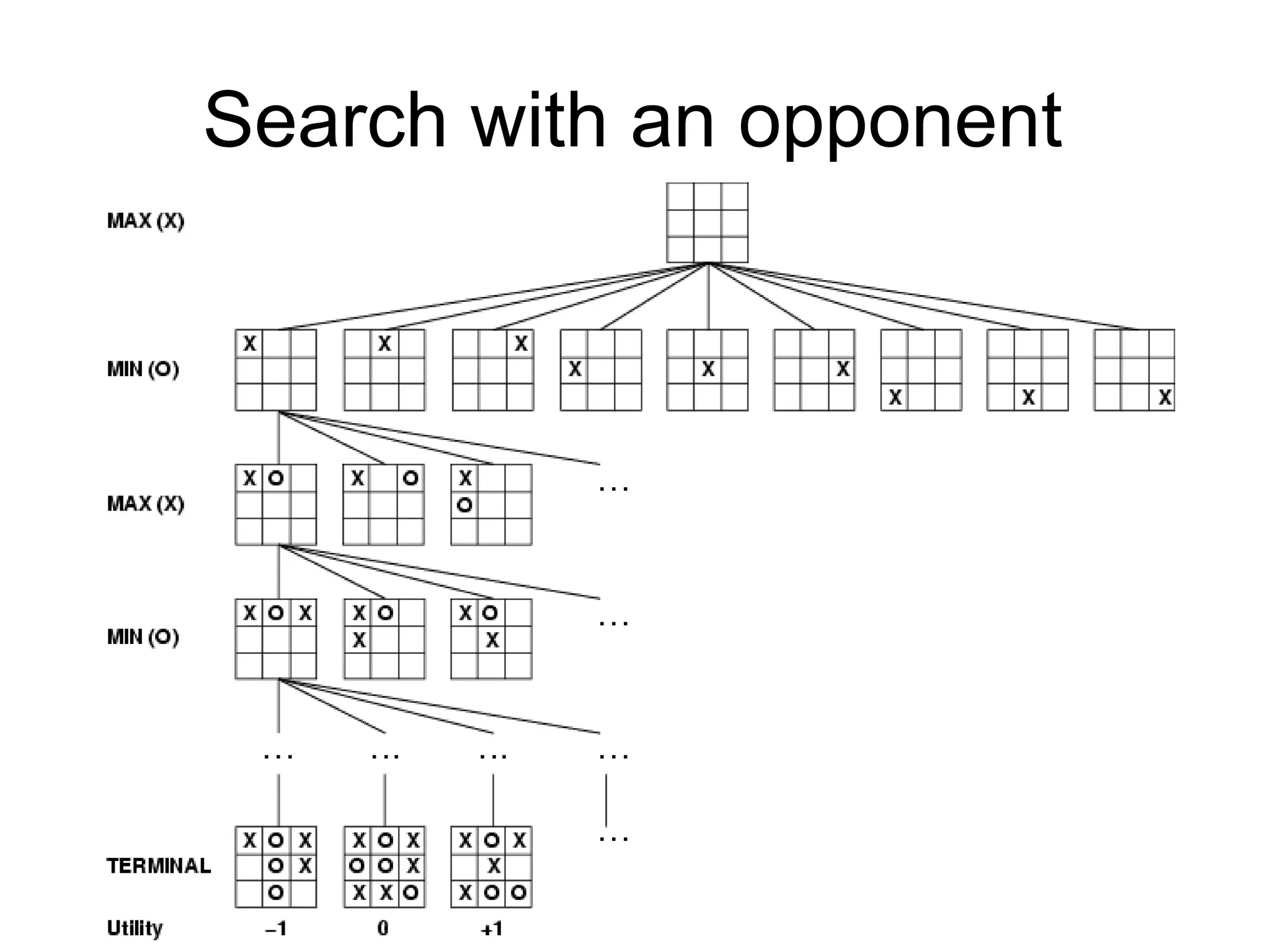
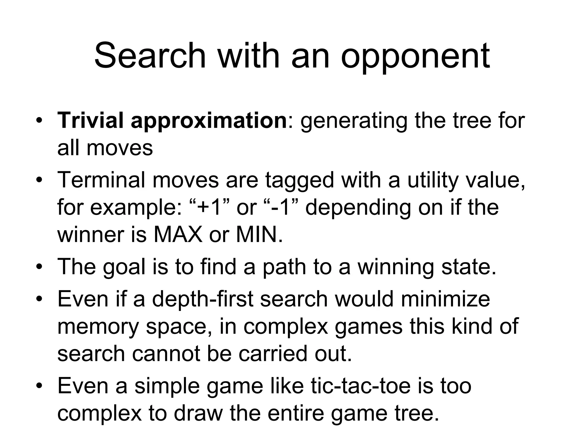
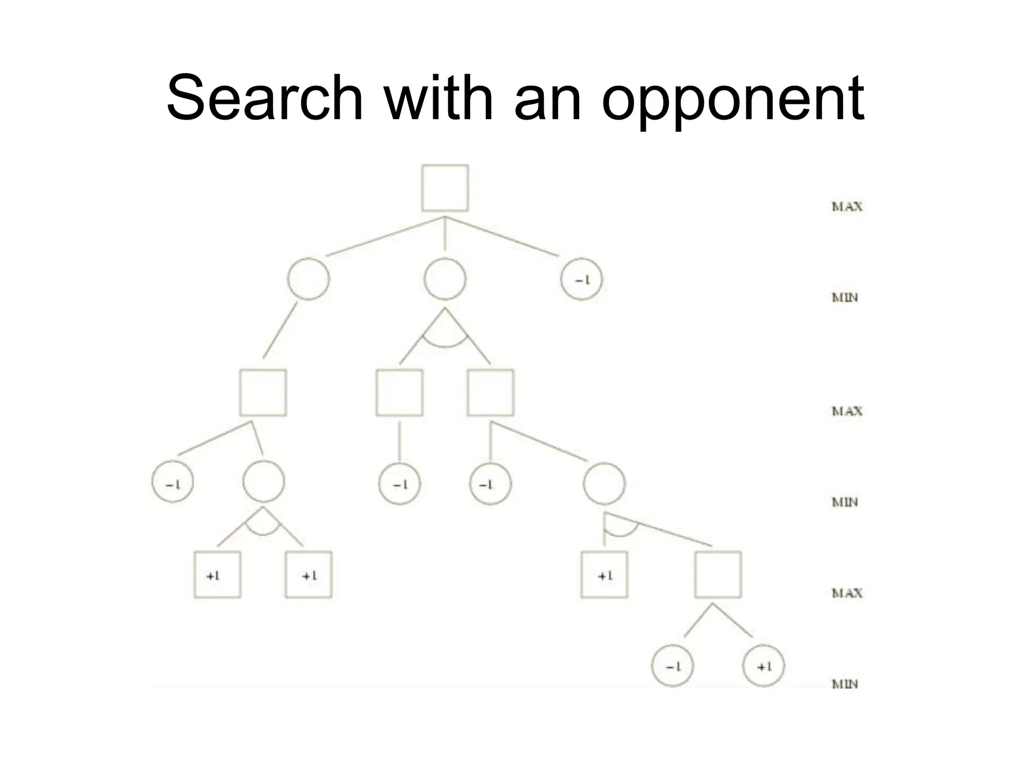
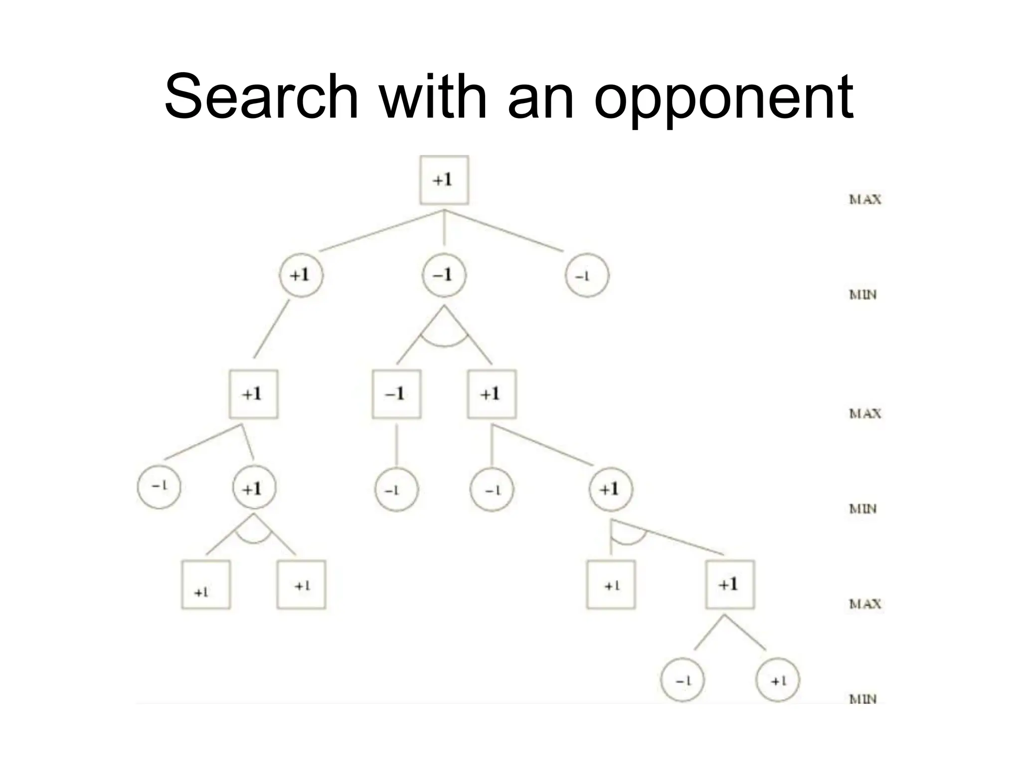
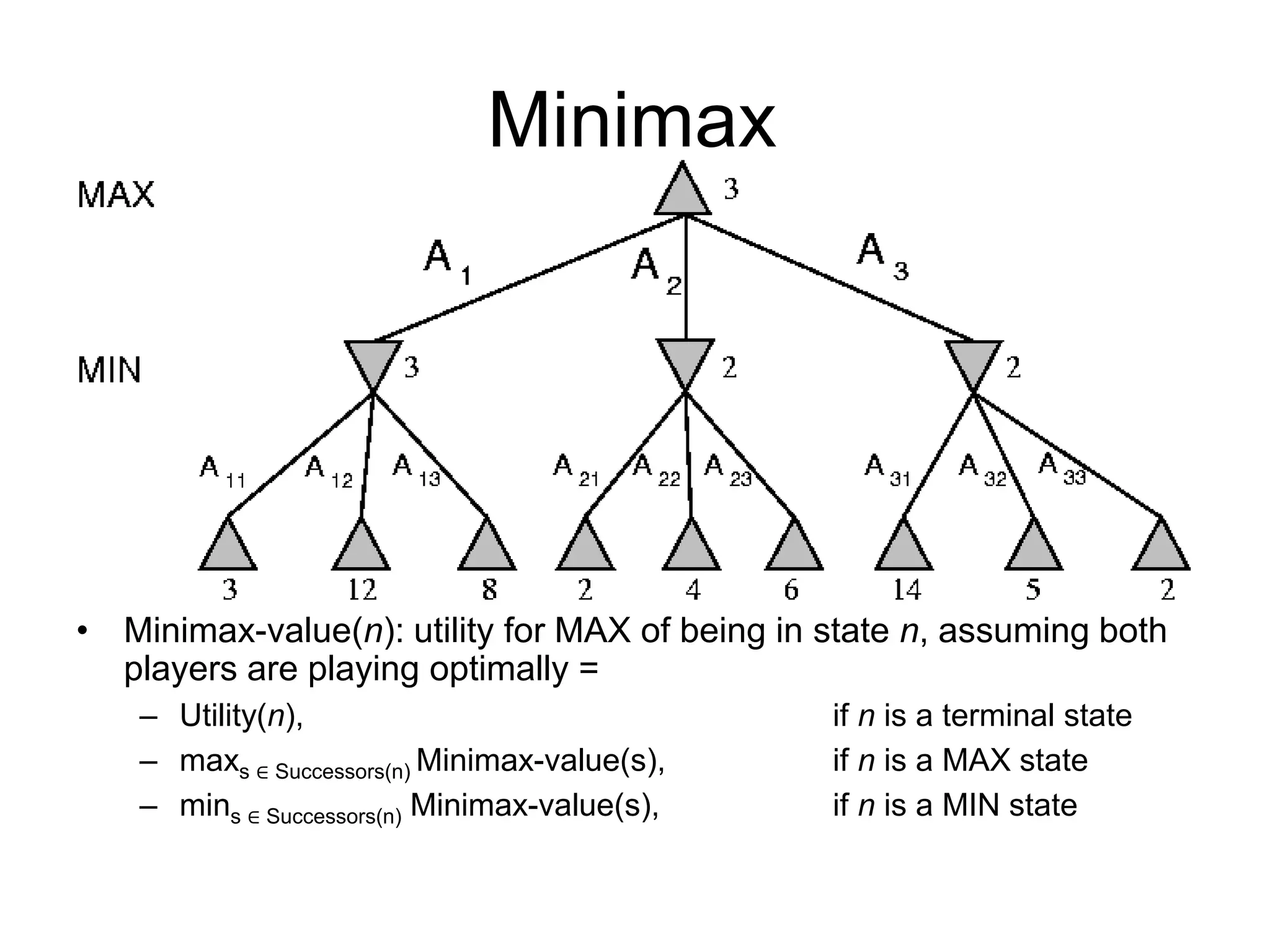
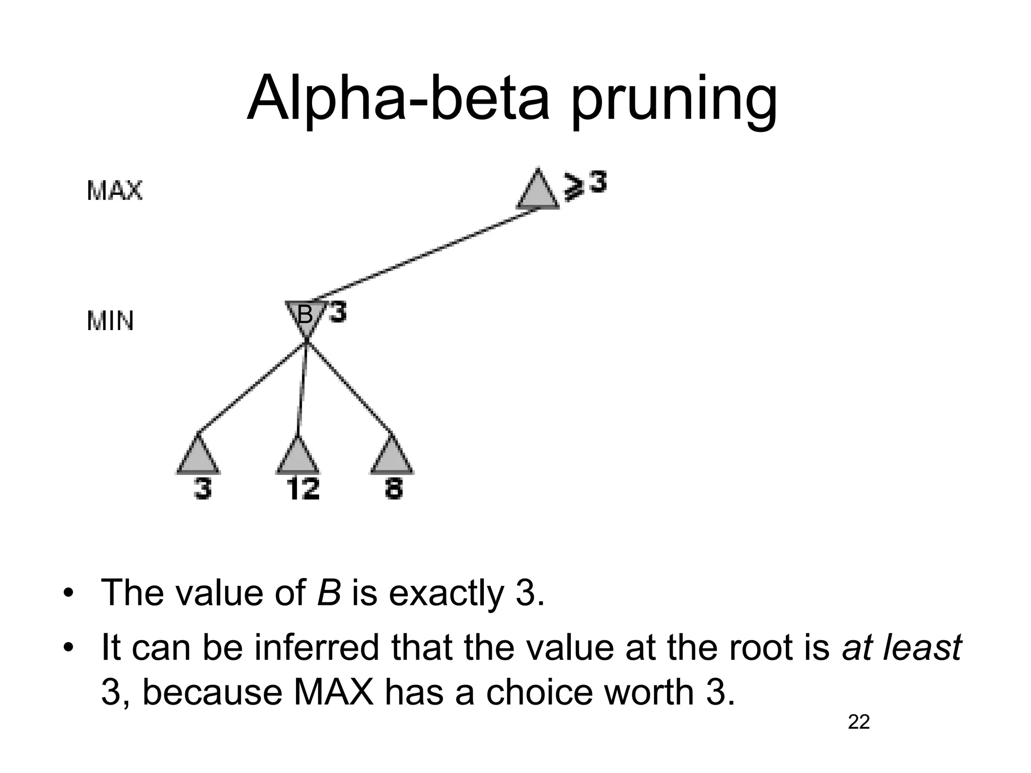
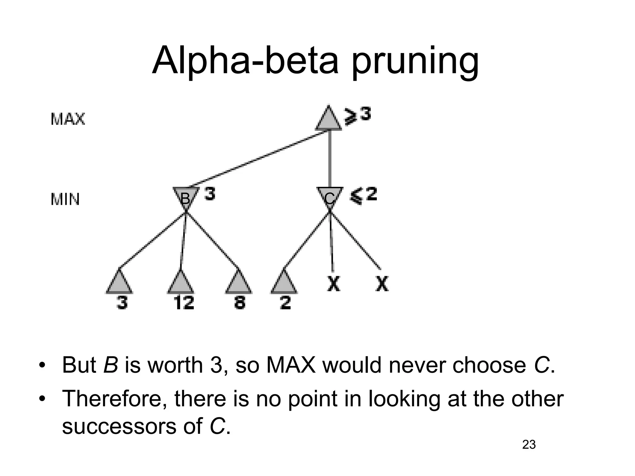
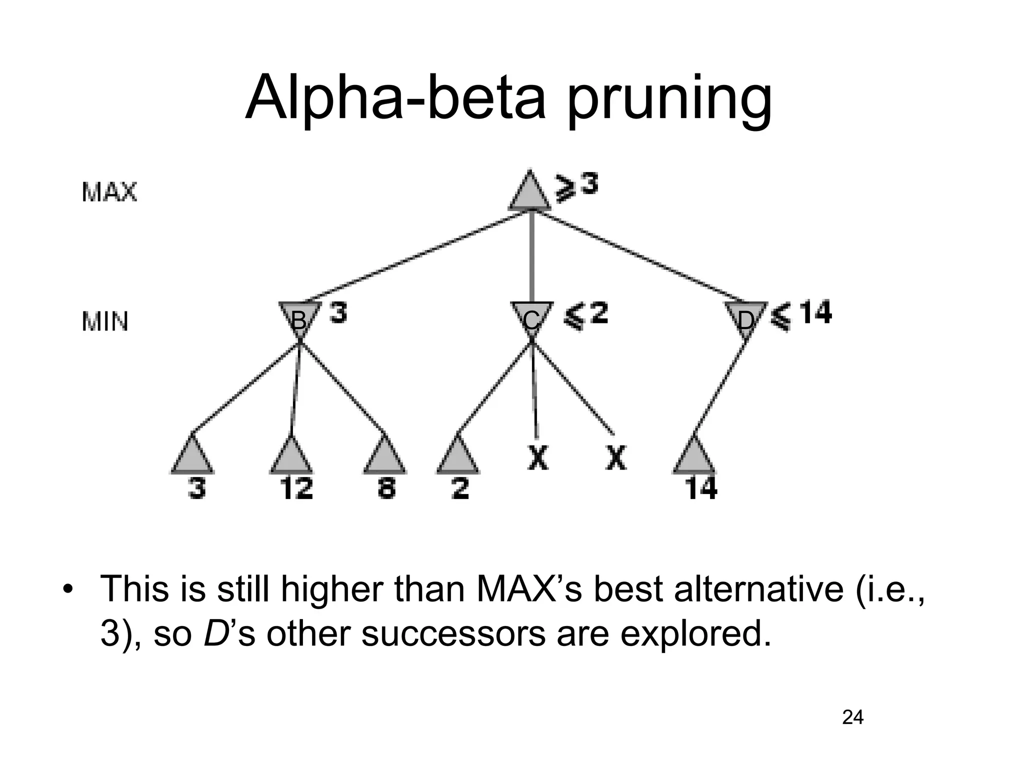
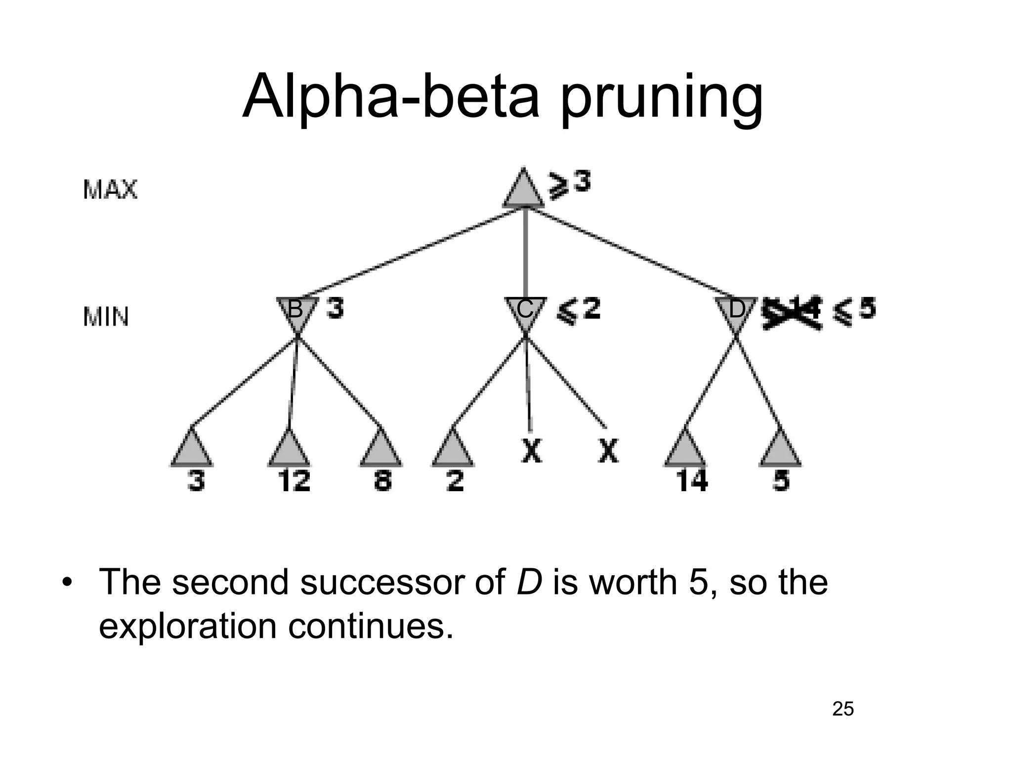
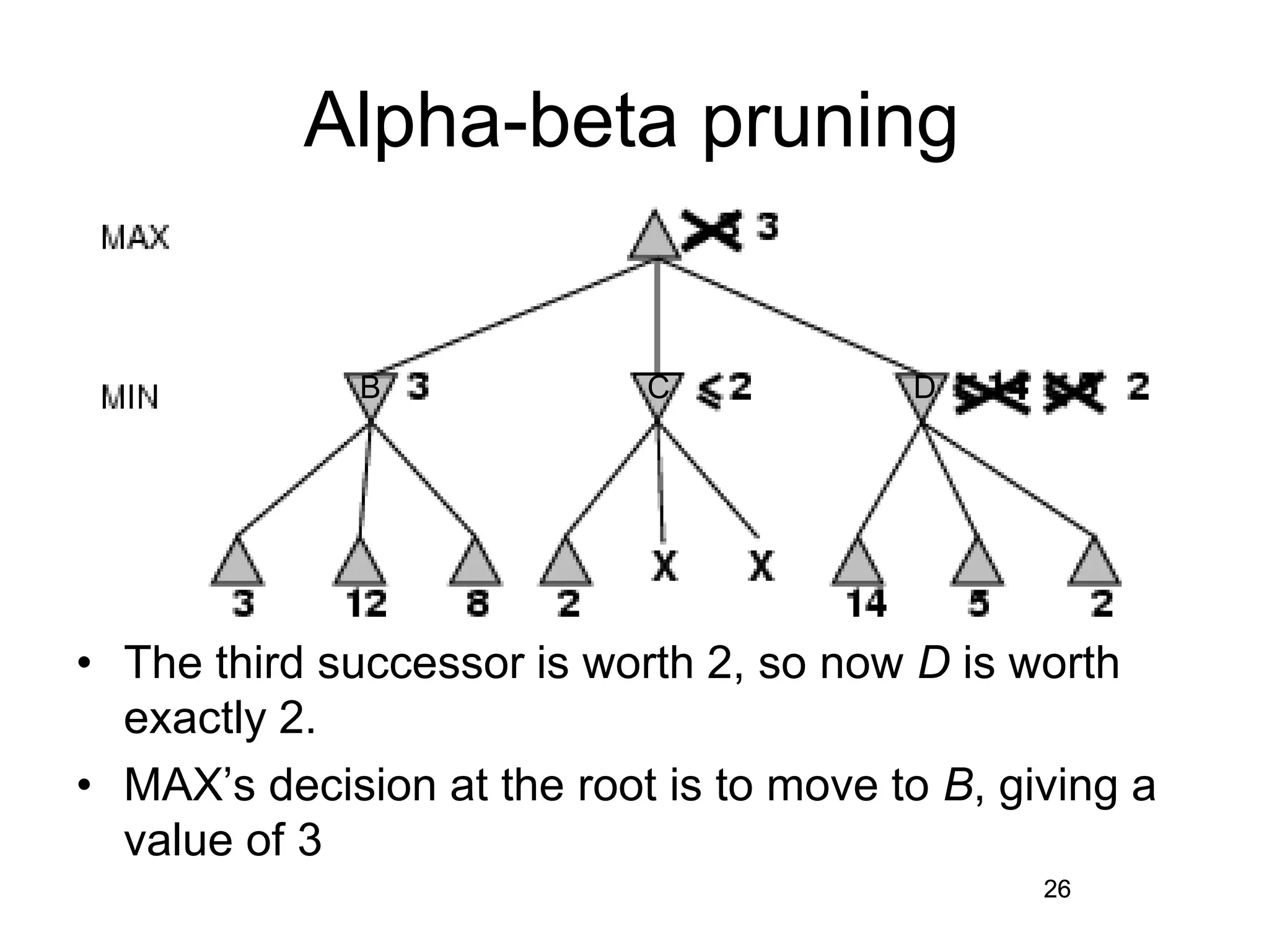
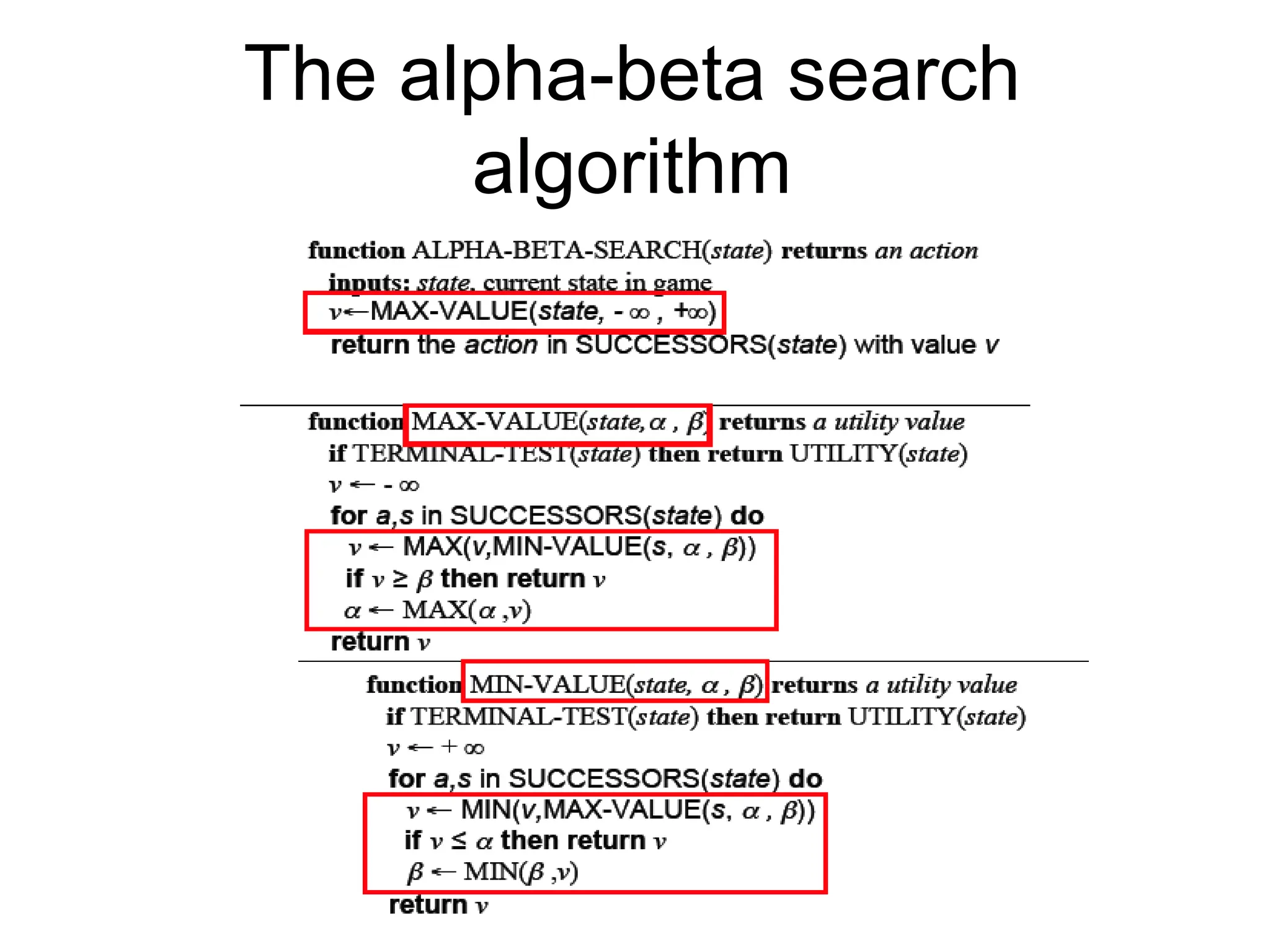
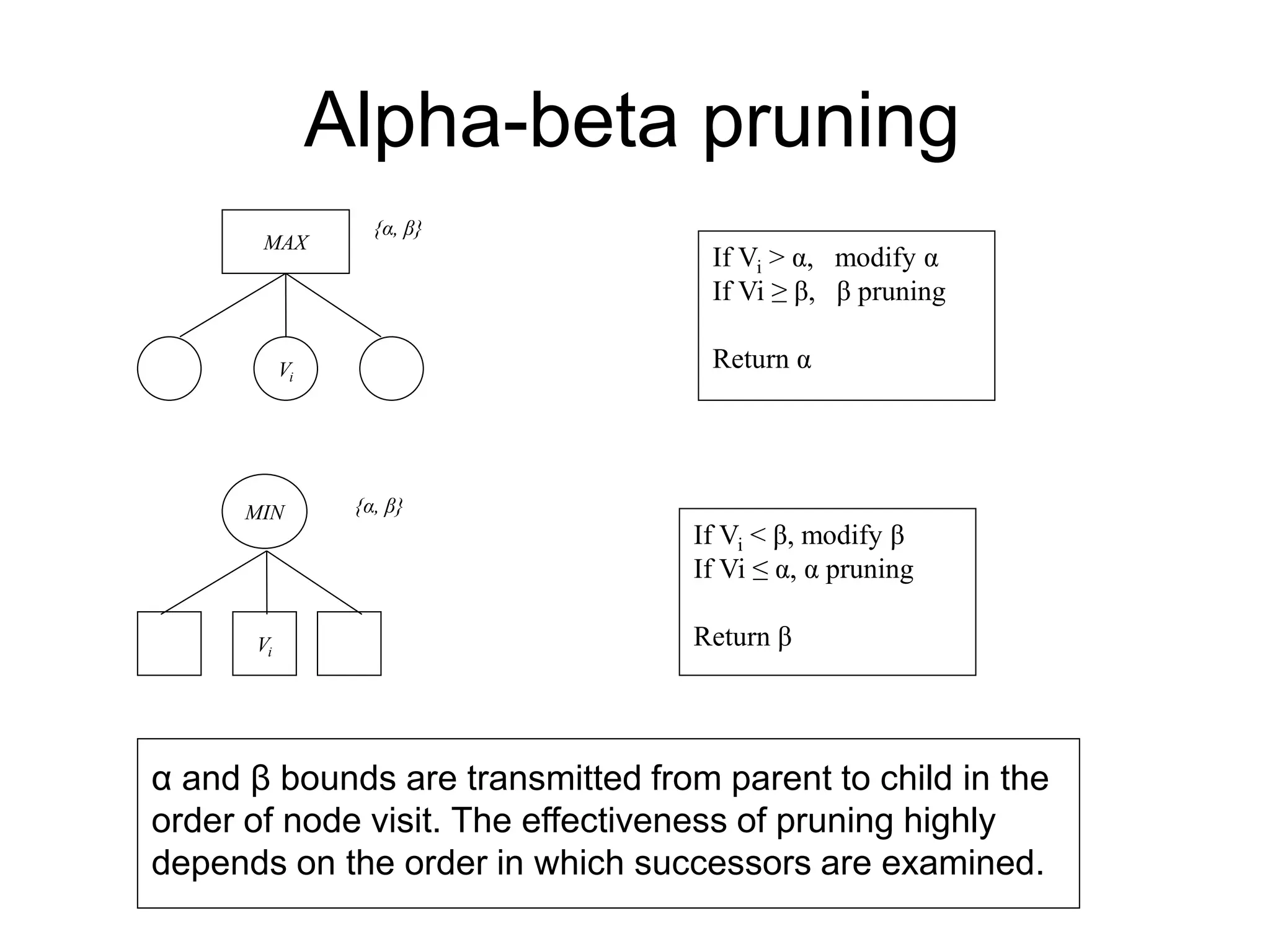
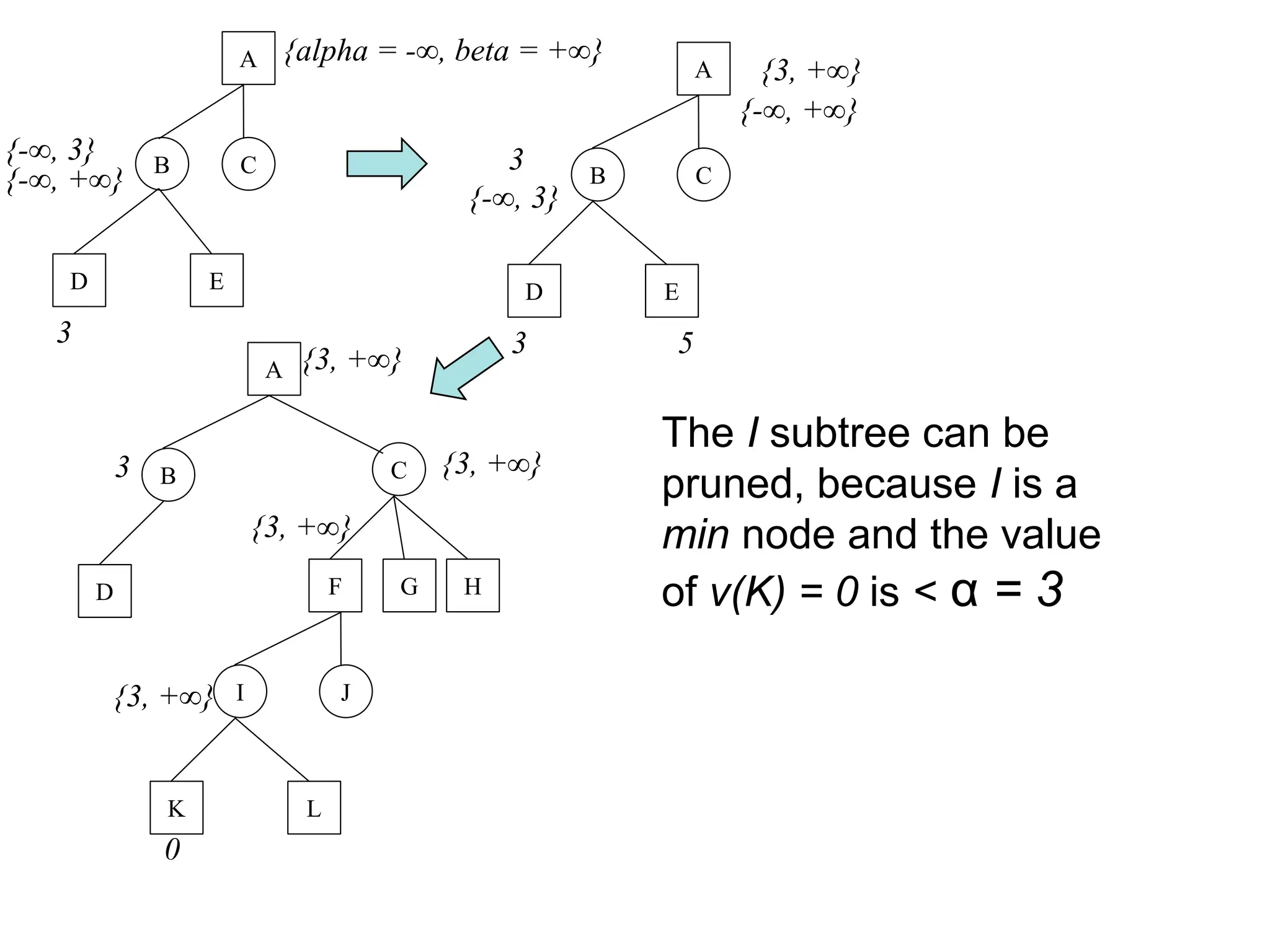
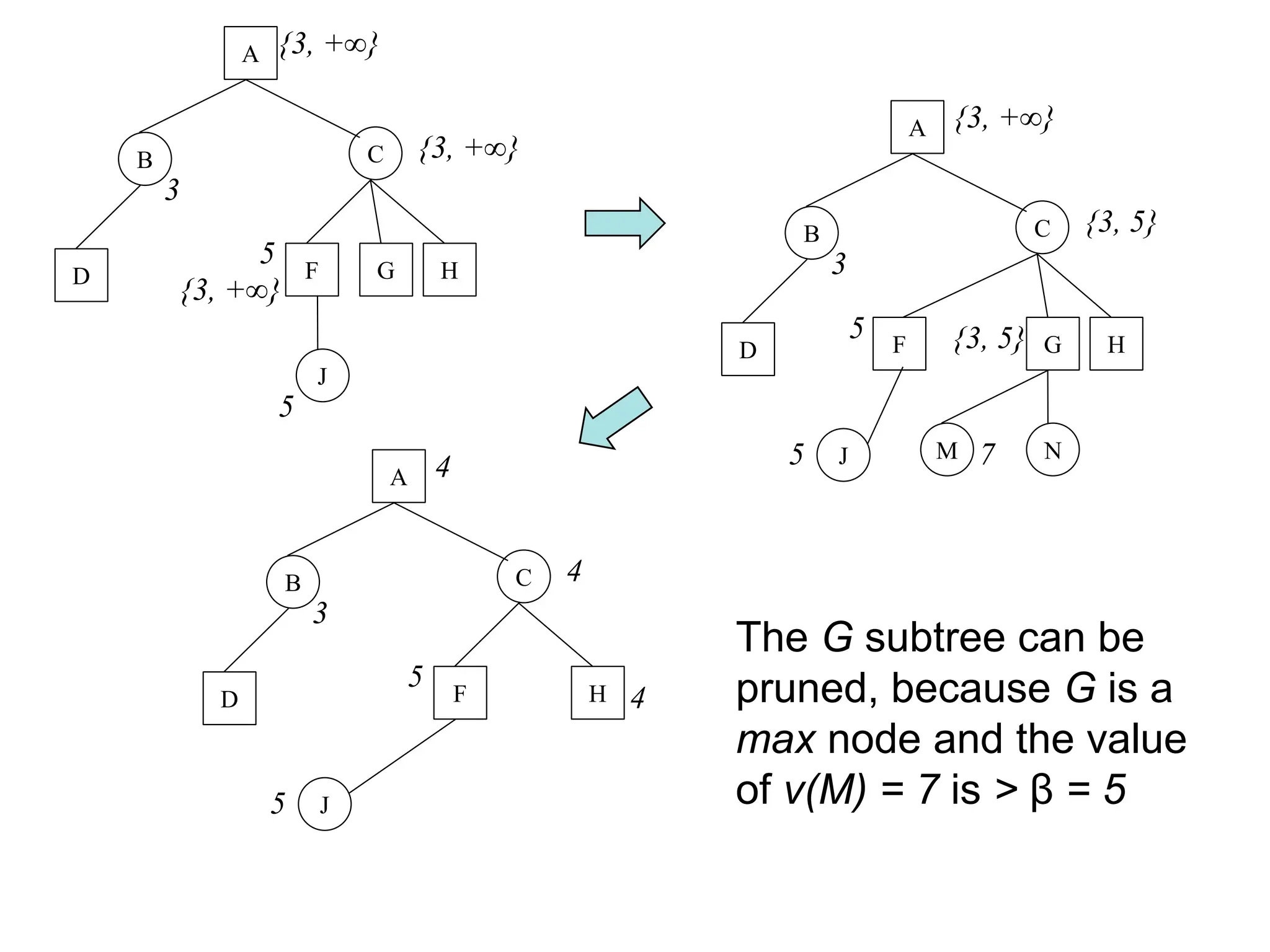
The document discusses adversarial search in artificial intelligence, focusing on game theory frameworks involving two players with alternate moves and perfect or imperfect information. Key concepts include the minimax algorithm, which recursively calculates values for each game state to find optimal moves, and alpha-beta pruning, which optimizes this process by eliminating branches that won't affect the final decision. The effectiveness of alpha-beta pruning is influenced by the order of examining successors, potentially reducing the time complexity of the search.

1. Artificial Intelligence
Adversarial search

2. Planning ahead in a world that
includes a hostile agent
• Games as search problems
• Idealization and simplification:
– Two players
– Alternate moves
• MAX player
• MIN player
– Available information:
• Perfect: chess, chequers, tic-tac-toe… (no chance,
same knowledge for the two players)
• Imperfect: poker, Stratego, bridge…

3. Game representation
• In the general case of a game with two
players:
– General state representation
– Initial-state definition
– Winning-state representation as:
• Structure
• Properties
• Utility function
– Definition of a set of operators

4. Search with an opponent

5. Search with an opponent
• Trivial approximation: generating the tree for
all moves
• Terminal moves are tagged with a utility value,
for example: “+1” or “-1” depending on if the
winner is MAX or MIN.
• The goal is to find a path to a winning state.
• Even if a depth-first search would minimize
memory space, in complex games this kind of
search cannot be carried out.
• Even a simple game like tic-tac-toe is too
complex to draw the entire game tree.

6. Search with an opponent

7. Search with an opponent

8. Search with an opponent
• Heuristic approximation: defining an evaluation
function which indicates how close a state is from a
winning (or losing) move
• This function includes domain information.
• It does not represent a cost or a distance in steps.
• Conventionally:
– A winning move is represented by the value“+∞”.
– A losing move is represented by the value “-∞”.
– The algorithm searches with limited depth.
• Each new decision implies repeating part of the search.

9. Minimax
• Minimax-value(n): utility for MAX of being in state n, assuming both
players are playing optimally =
– Utility(n), if n is a terminal state
– maxs ∈ Successors(n) Minimax-value(s), if n is a MAX state
– mins ∈ Successors(n) Minimax-value(s), if n is a MIN state

10. Example: tic-tac-toe
• e (evaluation function → integer) =
number of available rows, columns,
diagonals for MAX - number of available
rows, columns, diagonals for MIN
• MAX plays with “X” and desires
maximizing e.
• MIN plays with “0” and desires minimizing
e.
• Symmetries are taken into account.
• A depth limit is used (2, in the example).

11. Example: tic-tac-toe

12. Example: tic-tac-toe

13. Example: tic-tac-toe

14. 14
The minimax algorithm
• The minimax algorithm computes the
minimax decision from the current state.
• It uses a simple recursive computation of the
minimax values of each successor state:
– directly implementing the defining equations.
• The recursion proceeds all the way down to
the leaves of the tree.
• Then the minimax values are backed up
through the tree as the recursion unwinds.
14

15. 15
The minimax algorithm

16. 16
The minimax algorithm
• The algorithm first recurses down to the
tree bottom-left nodes
– and uses the Utility function on them to
discover that their values are 3, 12 and 8.
16

17. 17
The minimax algorithm
• Then it takes the minimum of these
values, 3, and returns it as the backed-up
value of node B.
• Similar process for the other nodes. 17
B
A

18. 18
The minimax algorithm
• The minimax algorithm performs a
complete depth-first exploration of the
game tree.
• In minimax, at each point in the process,
only the nodes along a path of the tree are
considered and kept in memory.
18

19. 19
The minimax algorithm
• If the maximum depth of the tree is m, and
there are b legal moves at each point,
then the time complexity is O(bm).
• The space complexity is:
– O(bm) for an algorithm that generates all
successors at once
– O(m) if it generates successors one at a time.
19

20. 20
The minimax algorithm:
problems
• For real games the time cost of minimax is
totally impractical, but this algorithm
serves as the basis:
– for the mathematical analysis of games and
– for more practical algorithms
• Problem with minimax search:
– The number of game states it has to examine
is exponential in the number of moves.
• Unfortunately, the exponent can’t be
eliminated, but it can be cut in half. 20

21. 21
Alpha-beta pruning
• It is possible to compute the correct
minimax decision without looking at every
node in the game tree.
• Alpha-beta pruning allows to eliminate
large parts of the tree from consideration,
without influencing the final decision.
21

22. • The leaves below B have the values 3, 12 and 8.
• The value of B is exactly 3.
• It can be inferred that the value at the root is at least
3, because MAX has a choice worth 3.
22
B
Alpha-beta pruning
22

23. • C, which is a MIN node, has a value of at most 2.
• But B is worth 3, so MAX would never choose C.
• Therefore, there is no point in looking at the other
successors of C.
23
Alpha-beta pruning
23
B C

24. • D, which is a MIN node, is worth at most 14.
• This is still higher than MAX’s best alternative (i.e.,
3), so D’s other successors are explored.
24
Alpha-beta pruning
24
B C D

25. 25
• The second successor of D is worth 5, so the
exploration continues.
Alpha-beta pruning
25
B C D

26. 26
• The third successor is worth 2, so now D is worth
exactly 2.
• MAX’s decision at the root is to move to B, giving a
value of 3
Alpha-beta pruning
26
B C D

27. 27
Alpha-beta pruning
• Alpha-beta pruning gets its name from two
parameters.
– They describe bounds on the values that
appear anywhere along the path under
consideration:
• α = the value of the best (i.e., highest value)
choice found so far along the path for MAX
• β = the value of the best (i.e., lowest value) choice
found so far along the path for MIN
27

28. 28
Alpha-beta pruning
• Alpha-beta search updates the values of α
and β as it goes along.
• It prunes the remaining branches at a
node (i.e., terminates the recursive call)
– as soon as the value of the current node is
known to be worse than the current α or β
value for MAX or MIN, respectively.
28

29. 29
The alpha-beta search
algorithm

30. MAX
Vi
{α, β}
If Vi > α, modify α
If Vi ≥ β, β pruning
Return α
{α, β}
If Vi < β, modify β
If Vi ≤ α, α pruning
Return β
MIN
Vi
α and β bounds are transmitted from parent to child in the
order of node visit. The effectiveness of pruning highly
depends on the order in which successors are examined.
Alpha-beta pruning

31. The I subtree can be
pruned, because I is a
min node and the value
of v(K) = 0 is < α = 3
A
C
B
E
D
3
{-∞, +∞}
A
C
B
E
D
3 5
3
{-∞, 3}
A
C
B
D
3
H
F
{3, +∞}
G
J
I
L
K
{3, +∞}
{3, +∞}
{3, +∞}
0
{alpha = -∞, beta = +∞}
{-∞, 3}
{-∞, +∞}
{3, +∞}

32. The G subtree can be
pruned, because G is a
max node and the value
of v(M) = 7 is > β = 5
A
C
B
D
3
H
F
{3, +∞}
G
J
{3, +∞}
{3, +∞}
5
5
A
C
B
D
3
H
F
{3, +∞}
G
J
{3, 5}
5
5
N
M 7
A
C
B
D
3
H
F
4
J
4
{3, 5}
5
5
4

33. 33
Final comments about alpha-
beta pruning
• Pruning does not affect final results.
• Entire subtrees can be pruned, not just leaves.
• Good move ordering improves effectiveness of
pruning.
• With perfect ordering, time complexity is
O(bm/2).
– Effective branching factor of sqrt(b)
– Consequence: alpha-beta pruning can look twice as
deep as minimax in the same amount of time.
33