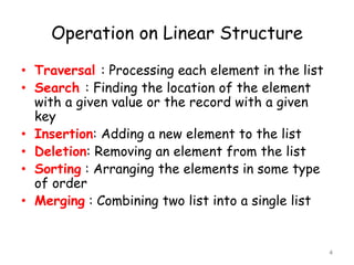
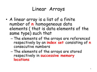
This document discusses data structures and algorithms. It begins by classifying data structures as linear or non-linear, with linear data structures having each element connected to a unique predecessor and successor. It then discusses the two basic representations of linear data structures in memory as either arrays or linked lists. Common operations on linear data structures like traversal, search, insertion, deletion, sorting, and merging are also outlined. The document proceeds to provide detailed explanations and examples of arrays, including linear arrays, representation in memory, traversing, inserting, deleting, and multidimensional arrays. It concludes with a brief discussion of pointers and pointer arrays.

1. Data Structure and Algorithm
CS-102/CS2005
1

2. Classification
• Data Structure
– Linear
– Non-Linear
A data structure is said to be linear if every
element in the data structure has a unique
successor and a unique predecessor other
than the first and last element. The first
element has no predecessor and the last
element has no successor.
2

3. Representation in Memory
• Two basic representation in memory
– Have a linear relationship between the
elements represented by means of
sequential memory locations [ Arrays]
– Have the linear relationship between the
elements represented by means of pointer
or links [ Linked List]
3

4. Operation on Linear Structure
• Traversal : Processing each element in the list
• Search : Finding the location of the element
with a given value or the record with a given
key
• Insertion: Adding a new element to the list
• Deletion: Removing an element from the list
• Sorting : Arranging the elements in some type
of order
• Merging : Combining two list into a single list
4

5. Array
5

6. Linear Arrays
• A linear array is a list of a finite
number of n homogeneous data
elements ( that is data elements of the
same type) such that
– The elements of the arrays are referenced
respectively by an index set consisting of n
consecutive numbers
– The elements of the arrays are stored
respectively in successive memory
locations
6

7. Linear Arrays
• The number n of elements is called the
length or size of the array.
• The index set consists of the integer 1,
2, … n
• Length or the number of data elements of
the array can be obtained from the index
set by
Length = UB – LB + 1 where UB is the
largest index called the upper bound and
LB is the smallest index called the lower
bound of the arrays
7

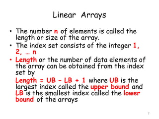
8. Linear Arrays
• Element of an array A may be denoted
by
– Subscript notation A1, A2, , …. , An
– Parenthesis notation A(1), A(2), …. , A(n)
– Bracket notation A[1], A[2], ….. , A[n]
• The number K in A[K] is called subscript
or an index and A[K] is called a
subscripted variable
8

9. Representation of Linear Array in Memory
9
1000
1001
1002
1003
1004
1005
Computer Memory
:

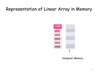
10. Representation of Linear Array in Memory
• Let LA be a linear array in the memory of
the computer
• LOC(LA[K]) = address of the element
LA[K] of the array LA
• The element of LA are stored in the
successive memory cells
• Computer does not need to keep track of
the address of every element of LA, but
need to track only the address of the first
element of the array denoted by Base(LA)
called the base address of LA
10

11. Representation of Linear Array in Memory
• LOC(LA[K]) = Base(LA) + w(K – LB)
where w is the number of words per
memory cell of the array LA [w is the
size of the data type]
11

12. Example 1
12
200
201
202
203
204
205
206
207
LA[0]
LA[2]
LA[3]
LA[4]
LA[5]
LA[6]
LA[7]
LA[1]
Find the address for LA[6]
Each element of the array
occupy 1 byte
LOC(LA[K]) = Base(LA) + w(K – lower bound)
LOC(LA[6]) = 200 + 1(6 – 0) = 206
:

13. Example 2
13
200
201
202
203
204
205
206
207
LA[0]
LA[1]
LA[2]
LA[3]
Find the address for LA[15]
Each element of the array
occupy 2 bytes
LOC(LA[K]) = Base(LA) + w(K – lower bound)
LOC(LA[15]) = 200 + 2(15 – 0) = 230
:

14. Representation of Linear Array in Memory
• Given any value of K, time to calculate
LOC(LA[K]) is same
• Given any subscript K one can access and
locate the content of LA[K] without
scanning any other element of LA
• A collection A of data element is said to be
indexed if any element of A called Ak can
be located and processed in time that is
independent of K
14

15. Traversing Linear Arrays
• Traversing is accessing and processing
each element of the data structure
exactly once.
15
•••
Linear Array

16. Traversing Linear Arrays
• Traversing is accessing and processing
each element of the data structure
exactly once.
16
•••
Linear Array

17. Traversing Linear Arrays
• Traversing is accessing and processing
each element of the data structure
exactly once.
17
•••
Linear Array

18. Traversing Linear Arrays
• Traversing is accessing and processing
each element of the data structure
exactly once.
18
•••
Linear Array

19. Traversing Linear Arrays
• Traversing is accessing and processing
each element of the data structure
exactly once.
19
•••
Linear Array

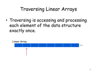
20. Traversing Linear Arrays
• Traversing is accessing and processing
each element of the data structure
exactly once.
20
•••
Linear Array
1. Repeat for K = LB to UB for( i=0;i<size;i++)
Apply PROCESS to LA[K] printf(“%d”,LA[i]);
[End of Loop]
2. Exit

21. Inserting and Deleting
• Insertion: Adding an element
– Beginning
– Middle
– End
• Deletion: Removing an element
– Beginning
– Middle
– End
21

22. Insertion
1 Brown
2 Davis
3 Johnson
4 Smith
5 Wagner
6
7
8
22
1 Brown
2 Davis
3 Johnson
4 Smith
5 Wagner
6 Ford
7
8
Insert Ford at the End of Array

23. Insertion
1 Brown
2 Davis
3 Johnson
4 Smith
5 Wagner
6
7
8
23
1 Brown
2 Davis
3 Johnson
4 Smith
5
6 Wagner
7
8
Insert Ford as the 3rd Element of Array
1 Brown
2 Davis
3 Johnson
4
5 Smith
6 Wagner
7
8
1 Brown
2 Davis
3
4 Johnson
5 Smith
6 Wagner
7
8
Ford
Insertion is not Possible without loss
of data if the array is FULL

24. Insertion Algorithm
• INSERT (LA, N , K , ITEM) [LA is a
linear array with N elements and K is a positive
integers such that K ≤ N. This algorithm inserts an
element ITEM into the Kth position in LA ]
1. [Initialize Counter] Set J := N
2. Repeat Steps 3 and 4 while J ≥ K
3. [Move the Jth element downward ] Set LA[J + 1]
:= LA[J]
4. [Decrease Counter] Set J := J -1
5 [Insert Element] Set LA[K] := ITEM
6. [Reset N] Set N := N +1;
7. Exit
24

25. Deletion
1 Brown
2 Davis
3 Ford
4 Johnson
5 Smith
6 Taylor
7 Wagner
8
25
1 Brown
2 Davis
3 Ford
4 Johnson
5 Smith
6 Taylor
7
8
Deletion of Wagner at the End of Array

26. Deletion
1 Brown
2 Davis
3 Ford
4 Johnson
5 Smith
6 Taylor
7 Wagner
8
26
1 Brown
2
3 Ford
4 Johnson
5 Smith
6 Taylor
7 Wagner
8
Deletion of Davis from the Array
1 Brown
2 Ford
3
4 Johnson
5 Smith
6 Taylor
7 Wagner
8
1 Brown
2 Ford
3 Johnson
4
5 Smith
6 Taylor
7 Wagner
8

27. Deletion
1 Brown
2 Ford
3 Johnson
4 Smith
5 Taylor
6 Wagner
7
8
27
No data item can be deleted from an empty
array

28. Deletion Algorithm
• DELETE (LA, N , K , ITEM) [LA is a
linear array with N elements and K is a positive
integers such that K ≤ N. This algorithm deletes Kth
element from LA ]
1. Set ITEM := LA[K]
2. Repeat for J = K+1 to N:
[Move the Jth element upward] Set LA[J-1] :=
LA[J]
3. [Reset the number N of elements] Set N := N - 1;
4. Exit
28

29. Multidimensional Array
• One-Dimensional Array
• Two-Dimensional Array
• Three-Dimensional Array
29

30. Two-Dimensional Array
• A Two-Dimensional m x n array A is a
collection of m . n data elements such
that each element is specified by a pair
of integers (such as J, K) called
subscripts with property that
1 ≤ J ≤ m and 1 ≤ K ≤ n
The element of A with first subscript J
and second subscript K will be denoted
by AJ,K or A[J][K]
30

31. 2D Arrays
The elements of a 2-dimensional array a
is shown as below
a[0][0] a[0][1] a[0][2] a[0][3]
a[1][0] a[1][1] a[1][2] a[1][3]
a[2][0] a[2][1] a[2][2] a[2][3]

32. Rows Of A 2D Array
a[0][0] a[0][1] a[0][2] a[0][3] row 0
a[1][0] a[1][1] a[1][2] a[1][3] row 1
a[2][0] a[2][1] a[2][2] a[2][3] row 2

33. Columns Of A 2D Array
a[0][0] a[0][1] a[0][2] a[0][3]
a[1][0] a[1][1] a[1][2] a[1][3]
a[2][0] a[2][1] a[2][2] a[2][3]
column 0 column 1 column 2 column 3

34. 2D Array
• Let A be a two-dimensional array m x n
• The array A will be represented in the
memory by a block of m x n sequential
memory location
• Programming language will store array A
either
– Column by Column (Called Column-Major
Order) Ex: Fortran, MATLAB
– Row by Row (Called Row-Major Order) Ex: C,
C++ , Java
34

35. 2D Array in Memory
A Subscript
(1,1)
(2,1)
(3,1)
(1,2)
(2,2)
(3,2)
(1,3)
(2,3)
(3,3)
(1,4)
(2,4)
(3,4)
35
Column 1
Column 2
Column 3
Column 4
A Subscript
(1,1)
(1,2)
(1,3)
(1,4)
(2,1)
(2,2)
(2,3)
(2,4)
(3,1)
(3,2)
(3,3)
(3,4)
Row 1
Row 3
Row 2
Column-Major Order Row-Major Order

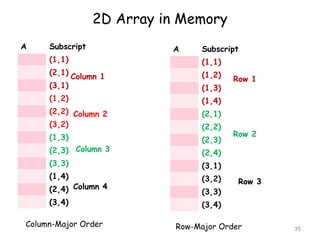
36. 2D Array
• LOC(LA[K]) = Base(LA) + w(K -1)
• LOC(A[J,K]) of A[J,K]
Column-Major Order
LOC(A[J,K]) = Base(A) + w[(J-LB) + m(K-LB)]
Row-Major Order
LOC(A[J,K]) = Base(A) + w[n(J-LB) + (K-LB) ]
36

37. 2D Array (Row Major)
A[J][K]
37
A5x6
Jth
Row
Kth
Column
LOC(A[J,K]) = Base(A) + w[n(J-LB) + (K-LB)]

38. 2D Array (Column Major)
A[J][K]
38
A5x6
Jth
Row
Kth
Column
LOC(A[J,K]) = Base(A) + w[(J-LB) + m(K-LB)]

39. Multidimensional Array
• Let C be a n-dimensional array
• Length Li of dimension i of C is the
number of elements in the index set
Li = UBi – LBi + 1
• For a given subscript Ki, the effective
index Ei of Ki is the number of indices
preceding Ki in the index set
Ei = Ki – LBi
39

40. Multidimensional Array
• Address LOC(C[K1,K2, …., Kn]) of an
arbitrary element of C can be obtained as
Column-Major Order
Base( C) + w[((( … (ENLN-1 + EN-1)LN-2)
+ ….. +E3)L2+E2)L1+E1]
Row-Major Order
Base( C) + w[(… ((E1L2 + E2)L3 + E3)L4
+ ….. +EN-1)LN +EN]
40

41. Example
• MAZE(2:8, -4:1, 6:10)
• Calculate the address of MAZE[5,-1,8]
• Given: Base(MAZE) = 200, w = 4, MAZE
is stored in Row-Major order
• L1 = 8-2+1 = 7, L2 = 6, L3 = 5
• E1 = 5 -2 = 3, E2 = 3, E3 = 2
41

42. Example Contd ..
• Base( C) + w[(… ((E1L2 + E2)L3 + E3)L4 +
….. +EN-1)LN +EN]
• E1L2 = 3 . 6 = 18
• E1L2 + E2 = 18 + 3 = 21
• (E1L2 + E2)L3 = 21 . 5 = 105
• (E1L2+E2)L3 + E3 = 105 + 2 = 107
• MAZE[5,-1,8] = 200 + 4(107) = 200 +
428 = 628
42

43. Pointer, Pointer Array
• Let DATA be any array
• A variable P is called a pointer if P points
to an element in DATA i.e if P contains
the address of an element in DATA.
e.g. int *p=&DATA[1];
• An array PTR is called a pointer array if
each element of PTR is a pointer
• int *PTR[5];
ptr[1] =&DATA[1];
ptr[2] =&DATA[2];
43