Downloaded 12 times


![9
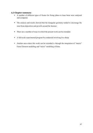
1.8.2 Apparent density remodelling
In this approach a continuous density distribution is defined throughout the bone. The
apparent density is defined as the ratio of the mass of bone inside a cubic element to the
volume of that cubic element (the element consists also of empty space, or in fact bone
marrow). This is different from the actual density of the bone. The actual density of the bone
is defined as the ratio of the mass of the bone to the volume of the bone.
The apparent density can also be defined as a relative density in which a value of ‘0’
indicates the element is empty and a value of ‘1’ indicates that it consists of solid bone.
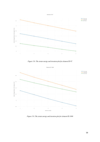
A differential equation is used to model the bone remodelling process. The bone model is
loaded for a multiple number of iterations. After each iteration, the apparent density
distribution in the bone is updated, based on the distribution of stress, strain and/or strain
energy within the bone. Usually, the strain energy density per unit mass or the average
absolute value of the principal strains is used as the bone remodelling parameter (Chen et al.,
2007, Huiskes et al., 1992). A threshold range of strain energy density values are defined. If
any element has a value above this threshold range, there will be an increase in density of that
element, and if the value is less than the threshold range there will be a decrease in density of
that element. This strain energy thresholding simulates an increase in density of the bone
(bone formation) and/or a decrease in density (bone loss).
Equation 1 shows the rate of change of apparent bone density:
d ρ
dt
= 𝐵 [
𝑆𝐸𝐷
ρ
− 𝑘]……………. Equation 1
where:
ρ apparent density
B is a constant controlling the rate of bone growth
SED strain energy density
𝑘 equilibrium level of strain energy per unit mass (which results in no bone growth)](https://image.slidesharecdn.com/4c8a10a2-b3da-430e-b419-1e05c2130871-151125122046-lva1-app6891/85/Aravind_Jayasankar_Master_Thesis-19-320.jpg)


![69
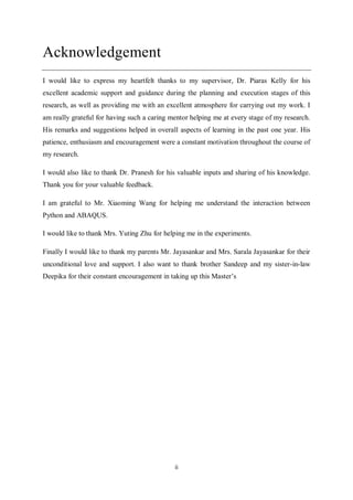
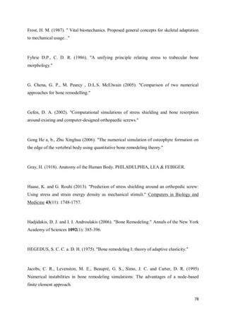
Appendix
Python script
from part import *
from material import *
from section import *
from assembly import *
from step import *
from interaction import *
from load import *
from mesh import *
from job import *
from sketch import *
from visualization import *
from connectorBehavior import *
from odbAccess import *
import numpy
# Accessing the .cae file and the bone part
mdb=openMdb('square_cortical')
model = mdb.models['Model-1']
partName = 'Bone'
corticalElementLabelList = []
corticalNodeLabelList = []](https://image.slidesharecdn.com/4c8a10a2-b3da-430e-b419-1e05c2130871-151125122046-lva1-app6891/85/Aravind_Jayasankar_Master_Thesis-79-320.jpg)
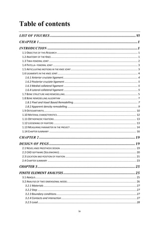
![70
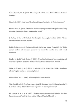
modelElements = model.parts[partName].elements
num_model_elements = len(modelElements)
print "CHECKING PROGRESS OF FINDING SURFACE ELEMENT NODE VERTICES"
index_list = [0,1,2]
# Finding the surface elements
for i, element in enumerate(modelElements):
adjacentElements = element.getAdjacentElements()
if len(adjacentElements) < 4:
curr_elem_edges = element.getElemEdges()
for edge in curr_elem_edges:
edgeNodes = edge.getNodes()
xCoords = [node.coordinates[0] for node in edgeNodes]
yCoords = [node.coordinates[1] for node in edgeNodes]
zCoords = [node.coordinates[2] for node in edgeNodes]
most_variant_dim = numpy.argmax([numpy.max(xCoords) -
numpy.min(xCoords), numpy.max(yCoords) - numpy.min(yCoords),
numpy.max(zCoords) - numpy.min(zCoords)])
coord_argmax_dim_list = [node.coordinates[most_variant_dim] for
node in edgeNodes]
temp_index_list = list(index_list)
temp_index_list.remove(numpy.argmax(coord_argmax_dim_list))
test_coord_argmax_dim_list = [coord_argmax_dim_list[j] for j in
temp_index_list]
test_coord_argmax_index =
numpy.argmax(test_coord_argmax_dim_list)](https://image.slidesharecdn.com/4c8a10a2-b3da-430e-b419-1e05c2130871-151125122046-lva1-app6891/85/Aravind_Jayasankar_Master_Thesis-80-320.jpg)
![71
remove_node_label =
edgeNodes[temp_index_list[test_coord_argmax_index]].label
for node in edgeNodes:
if node.label != remove_node_label:
corticalNodeLabelList.append(node.label)
del remove_node_label
print float(i)/num_model_elements
print "CHECKING PROGRESS OF FINDING SURFACE ELEMENTS"
# Elements attached to surface elements
for i, element in enumerate(modelElements):
curr_elem_edges = element.getElemEdges()
detect_node_list = []
for edge in curr_elem_edges:
edgeNodes = edge.getNodes()
xCoords = [node.coordinates[0] for node in edgeNodes]
yCoords = [node.coordinates[1] for node in edgeNodes]
zCoords = [node.coordinates[2] for node in edgeNodes]
most_variant_dim = numpy.argmax([numpy.max(xCoords) -
numpy.min(xCoords), numpy.max(yCoords) - numpy.min(yCoords),
numpy.max(zCoords) - numpy.min(zCoords)])
coord_argmax_dim_list = [node.coordinates[most_variant_dim] for
node in edgeNodes]
temp_index_list = list(index_list)
temp_index_list.remove(numpy.argmax(coord_argmax_dim_list))
test_coord_argmax_dim_list = [coord_argmax_dim_list[j] for j in
temp_index_list]](https://image.slidesharecdn.com/4c8a10a2-b3da-430e-b419-1e05c2130871-151125122046-lva1-app6891/85/Aravind_Jayasankar_Master_Thesis-81-320.jpg)
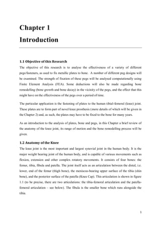
![72
test_coord_argmax_index = numpy.argmax(test_coord_argmax_dim_list)
remove_node_label =
edgeNodes[temp_index_list[test_coord_argmax_index]].label
# Creating sections for cortical and cancellous elements
for node in edgeNodes:
if (node.label != remove_node_label) and (node.label not in
detect_node_list):
detect_node_list.append(node.label)
del remove_node_label
all_nodes_in_list = 0
for nodeLabel in detect_node_list:
if nodeLabel in corticalNodeLabelList:
all_nodes_in_list += 1
elementLabel = str(element.label)
curr_elem_set = model.parts[partName].SetFromElementLabels('SET_' +
elementLabel, [element.label])
curr_elem_mat = mdb.models['Model-1'].Material('MAT_' +
elementLabel)
if all_nodes_in_list == 4:
corticalElementLabelList.append(element.label)
curr_elem_mat.Elastic(table =
model.materials['Cortical'].elastic.table)
else:
curr_elem_mat.Elastic(table =
model.materials['Bone'].elastic.table)
model.HomogeneousSolidSection(name = 'SEC_' + elementLabel,
material = 'MAT_' + elementLabel)](https://image.slidesharecdn.com/4c8a10a2-b3da-430e-b419-1e05c2130871-151125122046-lva1-app6891/85/Aravind_Jayasankar_Master_Thesis-82-320.jpg)
![73
model.parts[partName].SectionAssignment(sectionName = 'SEC_' +
elementLabel, region = curr_elem_set)
print float(i)/num_model_elements
model.parts['Bone'].SetFromElementLabels(name='corticalElementLabels
', elementLabels=corticalElementLabelList)
print "sections created";
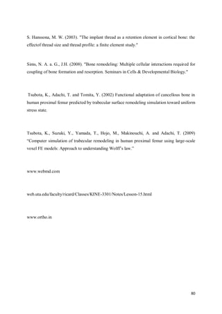
# Specifying number of loops the simulation should run
i=0
while(i<5):
print "job creating";
# printing job
# Naming the .odb file. The name of the file is followed by
iteration number
jobname = 'square_cortical_feb5_1' +str(i)
myJob = mdb.Job(name=jobname, model=model)
myJob.submit()
myJob.waitForCompletion()
odb=openOdb(jobname + '.odb')
print "job created";
eseden_values = odb.steps['Step-
1'].frames[1].fieldOutputs['ESEDEN'].values
print "eseden values read";
# Reading strain energy density values from .odb file
for eseden_val in eseden_values:
if partName.upper() in eseden_val.instance.name:
elementLabel = str(eseden_val.elementLabel)](https://image.slidesharecdn.com/4c8a10a2-b3da-430e-b419-1e05c2130871-151125122046-lva1-app6891/85/Aravind_Jayasankar_Master_Thesis-83-320.jpg)
![74
if eseden_val.elementLabel not in corticalElementLabelList:
eseden_data = eseden_val.data
# Defining the ESEDEN threshold values
if eseden_data > 0.00001:
curr_matProp_table = model.materials['MAT_' +
elementLabel].elastic.table
curr_E = curr_matProp_table[0][0]
curr_E += 10
curr_matProp_table = ((curr_E, curr_matProp_table[0][1]),)
model.Material('MAT_' + elementLabel).Elastic(table =
curr_matProp_table)
elif eseden_data < 0.000001:
curr_matProp_table = model.materials['MAT_' +
elementLabel].elastic.table
curr_E = curr_matProp_table[0][0]
curr_E -= 10
curr_matProp_table = ((curr_E, curr_matProp_table[0][1]),)
model.Material('MAT_' + elementLabel).Elastic(table =
curr_matProp_table)
print "property changed";
i=i+1
mdb.save()
print "cae saved";](https://image.slidesharecdn.com/4c8a10a2-b3da-430e-b419-1e05c2130871-151125122046-lva1-app6891/85/Aravind_Jayasankar_Master_Thesis-84-320.jpg)


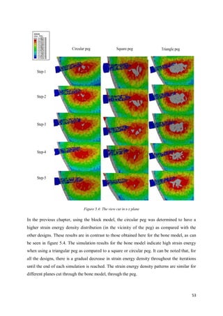
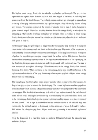
This document summarizes the design of attachments for a novel knee implant. It describes the design of three different peg shapes (circular, triangular, and square) to attach plates to the femur and tibia bones as part of a new knee prosthesis. Finite element analysis was performed using ABAQUS to simulate the performance of each peg design under loading conditions and over time. The results suggest that a triangular peg encourages higher bone formation compared to the other designs, as measured by strain energy density in the bone near the pegs.


