Aqt instructor-notes-final

LECTURES &
ADVANCED QUANTITATIVE TECHNIQUES NOTES

Lectures & Notes

ADVANCED QUANTITATIVE TECHNIQUES
(COURSE FOR PHD STUDENTS)

By
Dr. Anwar F. Chishti
Professor
Faculty of Management & Social
Sciences

1

LECTURES &

ADVANCED QUANTITATIVE TECHNIQUES

Course Plan
Fall Semester 2012
Course Instructor Professor Dr. Anwar F. Chishti
Contacts: Phone Phone: 0346-9096046
Email anwar@jinnah.edu.pk; chishti_anwar@yahoo.com
Class venue Computer Laboratory

Course contents
Topic 1: Simple/Two-Variable Regression Analysis:
• An introduction of estimated model and its interpretation,
• Regression Coefficients and Related Diagnostic Statistics:
Computational Formulas
• Evaluating the results of regression analysis
• Standard assumptions, BLUE properties of the estimator.
• Take-home assignment - 1
Topic 2: Simple Regression to Multiple Regression Analysis
• Shortcomings of simple/two-variables regression analysis
• An example of multiple regression analysis
• Use of Likert-scale type questionnaire, raw-data entry, reliability test
and generation of variables
• Estimation of multiple regression model
• Evaluation of the estimated model in terms of F-statistic, R2 and t-
statistic/p-value
Topic 3: Multiple Regression: Model specification
• 3.1(a) Conceiving research ideas and converting it into research
projects: a procedure
• 3.1(b) Incorporating theory as the base of your research: econometrics
theory & economics/management theory
• Take-home assignment – 3(a)
• 3.2 (a) Specification of an econometric model: mathematical
specification

2

LECTURES &

• 3.2(b) Some practical examples of mathematical specification:
production-function specification, cost-function specification, revenue-
function specification
• Take-home assignment – 3(b)
• 3.3(a) Conceptual/econometric modeling: (a) Examples in Finance; (b)
Examples in Marketing; (c) Examples in HRM
• 3.3(b) Incorporating theory as the base of your research: econometrics
theory & economics/management theory
• Take-home assignment: adopting, adapting and developing a new
questionnaire
Topic 4: Analyzing mean values
• Analyzing mean value, using one-sample t-test
• Comparing mean-differences of two or more groups
• Comparing two groups
* Independent samples t test
* Paired-sample t test
• Comparing more-than-two groups
* One-Way ANOVA
* Repeated ANOVA
• Take-home assignment – 4
Topic 5: Uses of estimated econometric models
• Some examples
Topic 6: Relaxing of Standard Assumptions: Normality Assumption and its testing
• Normality assumption
• Its testing
Topic 7: Problem of Multicollinearity: What Happens if Regressors are Correlated?
• Consequences, tests for detection and solutions/remedies
Topic 8: Problem of Heteroscadasticity: What Happens if the Error Variance is
nonconstant?
Topic 9: Problem of Autocorrelation: What Happens if the Error terms are
correlated?
Topic 10: Mediation and moderation analysis - I
• Estimating and testing mediation

3

LECTURES &

Topic 11: Mediation and moderation analysis - II
• Estimating and testing moderation
Topic 12: Time-series analysis - I
• Unit root analysis
Topic 13: Time-series analysis - II
• Unit root, co-integration and error correction modeling (ECM)
Topic 14 Panel data analysis, Simultaneous equation models/Structural equation
models
• Panl data analysis
• SEM, ILS, 2SLS and 3SLS
Topic 15 Qualitative response regression models (when dependent variables are
binary/dummy) and Optimization
• LPM, Logit model and Probit Model
• Take-home assignment – 13(a)
• * Optimization: minimization and maximization
• Take-home assignment – 13(b)
Topic 16 Welfare analysis: maximization of producer and consumer surpluses and
minimization of social costs

Required Text & Recommended Reading
The prescribed textbooks for this course are:

Gujarati, Damodar N. Basic Econometrics, 4th Edition. McGraw-Hill. 2007

Stock, J. H. and Watson, M.W. Introduction to Econometrics, 3/E. Pearson Education,
2011

Reference Books/Materials

Studenmund, A.H. Using Econometrics: A Practical Guide, 6/E, Prentice Hall

Asteriou, D. and Hall, S.G. Applied Econometrics – A Modern Approach. Palgrave
Macmillan, 2007.

4

LECTURES &

Andren, Thomas. (2007). Econometrics. Bookboon.com

Salvatore, D and Reagle, D. Statistics and Econometrics, 2nd Ed. Schaum’s Outlines.

Instructor’s class-notes (hard copy at photo-copier shop)

Assessment Criteria

Details Due Date Weighting
10 best weekly assignments (out of total
Individual Assignments 13 - 15, each having 2 marks) will be 20 %
counted toward total 20% marks.
A group of 2 students will select a topic,
Group research on selected carry out research, complete a research
20 %
research topics study, and make presentation in during
the last classes of the semester
Mid-term Examination As per University’s announcement 20 %
Final Examination As per University’s announcement 40 %
Total marks: 100

5

LECTURES &

Topic 1
Simple/Two-Variable Regression Analysis
1.1 Simple regression analysis: an example
Assuming a survey of 10 families yields the following data on their consumption expenditure (Y)
and income (X).
Y (Thousands) X (Thousands)
70 80
65 100
90 120
95 140
110 160
115 180
120 200
140 220
155 240
150 260
The theory suggests that families’ consumption (Y) depends on their income (X); hence,
econometric model may be specified, as follows.
Y = f(X) (General form) (1a)
Or Y = β0 + β1X + e (Linear form) (1b)
The above stated regression analysis model contains two variables (one independent variable X
and one dependent variable Y); this model is therefore called Two-variables or Simple
regression analysis model.
Is this type of Simple or Two-variable model justified? We will discuss this question later on;
let’s first estimate this model, using the Statistical Package for Social Sciences’ software SPSS.
The estimated model & interpretation
Y = 24.4530 + 0.5091 X (2a)
(6.4140) (0.0357) (Standard Error) (2b)
(3.8124) (14.2445) (t-statistic) (2c)
(0.005) (0.000) (p-value/sig. level) (2d)

R= 0.981 R2 = 0.9621 R2adjusted = 0.957
F = 203.082 (p-value = 0.000) DW = 2.6809 N = 10 (2e)

1.2 Regression analysis: computational formulas
The econometric model specified in (1) is estimated in the form of estimated model (2a) along
with all its diagnostic statistics 2(b – e), using the formulas provided, as follows.

6

LECTURES &

The coefficients ßs
∧ ∧
β0 = Y − β1 X (3)
∧
β1 =
∑ ( Xi − X ) (Yi −Y )
(4)
∑ ( Xi − X )
2

∧
β1 =
∑x y i i
(5)
∑x
2
i

Variances (σ 2) and Standard Errors (S.E):
2
 ∧

∧
∑e
2 ∑Y

−Yi 

i
(6)
σ =2
=
( N − 2) ( N − 2)
∧
Var ( β 0 ) = σ
∧
2
=
∑ X .σ i
2 2

(7)
N ∑x
β0 2
i

∧ ∧ ∧
S .E ( β0 ) = σ β0 = σ β0
2 (8)
∧ ∧
σ2
Var ( β1 ) = σ β1 =
2
(9)
∑x 2
i

∧ ∧ ∧
S .E ( β1 ) = σ β1 = σ β1
2 (10)
T-ratios:
∧
β0
Tβ0 = ∧ (11)
σβ 0

∧
β1
Tβ1 = ∧
σβ 11

(12)
The Coefficient of Determination ( R2 ):
 ∧

ESS ∑Y


i −Y 

R2 = =
TSS (
∑Y i −Y )
(13)
RSS
= 1−
TSS

=1 −
∑ e 2
i

∑Y −Y )
( 2
i

F – Statistics:

F =
ESS df
=
( R ) ( K −1)2

RSS df (1 − R ) ( N − K ) 2

(14)

7

LECTURES &

Durban-Watson (D.W) Statistics:
2

∑(e − et −1 )
N

t
t =2
d = N

∑e
t =1
2
t

(15)

1.3 Estimation of the model using computational formulas
We now use formula provided in (3) to (15), make computations like Table 3.3 (Gujarati,
2007) and resolve the model, as follows.
Yi = ßo + ß1 Xi + ℮i …….. Linear model (16)
Regression Coefficients ( ß i ):
ˆ
β1 =
∑ xi . yi = 16800 = 0.5091
(17)
∑ xi2 33000
∧ ∧
β0 = Y − β1 X = 111 − 0.5091 (170 )
(18)
= 24.453
Variances (σ 2) and Standard Errors (S.E):
∑e
2
∧
337.25
σ = 2
= = 42.15625 (19)
( N − 2) 10 − 2
∧
Var ( β0 ) = σβ
∧
2
=
∑X .σ i
2 2

=
( 322,000 ) ( 42.15625)
0
N ∑x 2
i ( 10 ) ( 33,000 )

= 41.13428
(20)
∧ ∧ ∧
S .E ( β0 ) = σ β0 = σ β0
2
= 41.13428 = 6.4140
(21)
∧ ∧
σ2
ˆ 42.15625
Var ( β1 ) = σ β1 = 2
= = 0.001277
∑x 2
i 33,000
(22)
∧ ∧ ∧
S .E ( β1 ) = σ β1 = σ β1
2
= 0.001277 = 0.03574
(23)

T-ratios:

8

LECTURES &

∧
β0 42.453
Tβ0 = ∧
= = 3.8124
σβ 6.414
0

(24)
∧
β1 0.5091
Tβ1 = ∧
= = 14.2445
σβ 0.03574
11

(25)
The Coefficient of Determination ( R2 ):

R 2 = 1−
∑e 2
i
=1 −
337.25
= 0.9621
∑(Y −Y )
2
8890
i

(26)
F – Statistics:
F=
( R ) ( K − 1)
2
=
0.9621 ( 2 − 1 )
(1 − R ) ( N − K )
2
0.0379 (10 − 2 )
(27)
0.9621
= = 203.082
0.0047375
The estimated model:
Y = 24.4530 + 0.5091X
(6.414) (0.0357)  S.E.
(3.812) (14.244)  t-ratio
(0.005) (0.0000) (p-valuel)

R2 = 0.9621 F = 203.082 N = 10 (28)

1.4 Regression analysis: the underlying theory
The above reported formulas reflect how various needed computations are carried out in
regression analysis. Specifically, formula (4) estimates the coefficient (β 1) of explanatory
variable X:
∧
β1 =
∑ ( Xi − X ) (Yi −Y )
∑ ( Xi − X )
2

That is: ‘the deviations of individual observation on Xi from its mean, multiplied by deviations of
respective Yi from its mean (cross-deviation), divided by the squares of the variations of Xi’; so
it is the ratio between cross-deviations of X – Y variables and X variable. Theoretically, β1

9

LECTURES &

measures ‘total cross deviations/variations per unit of variation in X-variable’. The intercept β0
measures ‘mean value of Y minus total contribution of mean of X’.
∧ ∧
β0 = Y − β1 X

1.5 Error term: its estimation and importance
When an econometric model, like 1(b), is specified:
Y = β0 + β1X + e (29a)

It contains an error or residual term (e); but when model is estimated like 2(a):
Y = 24.4530 + 0.5091X (29b)
The error term (e) seems to disappear; where does the error term go?
In fact the estimated model like 29(b) is valid only for the mean/average values of X and Y, and
equality in 29(b) does not hold when values other-than-mean values are used; we can compute
values of error terms or residuals, using the following formula.
Yi – Ŷ = e (30a)
Yi – (24.4530 + 0.5091Xi) = e (30b)
Putting individual-observation values from the original data, that is:
Y X
70 80
65 100
90 120
95 140
110 160
115 180
120 200
140 220
155 240
150 260

Yi – (24.4530 + 0.5091Xi) = e
70 – (24.4530 + 0.5091*80 = 4.8181 (30c)
65 – (24.4530 + 0.5091*100) = -10.3636 (30d)
90 – (24.4530 + 0.5091*120 = 4.4545 (30e)
95 – (24.4530 + 0.5091*140) = -0.7272 (30f)
110 – (24.4530 + 0.5091*160) = 4.0909 (30g)

10

LECTURES &

115 – (24.4530 + 0.5091*180) = -1.0909 (30i)
120 – (24.4530 + 0.5091*200) = -6.2727 (30j)
140 – (24.4530 + 0.5091*220) = 3.5454 (30k)
155 – (24.4530 + 0.5091*240) = 8.3636 (30l)
150 – (24.4530 + 0.5091*260) = -6.8181 (30m)
As reflects from the above computations, error term reflects how much an individual Y deviates
from its estimated value. The values of error terms play important role in determining the size of
variance Ϭ2 (computational formula 6), which further affects a number of other computations.
A characteristic of error or residual term is that, once we add or take its mean value, it turns out
equal to zero, in both cases.

1.6 Evaluating the estimated model
After running regression, the results are reported usually reported in the following form.
Y = 24.4530 + 0.5091X (31a)
(6.4140) (0.0357) (Standard error) (31b)
(3.8124) (14.2445) (t-statistic) (31c)
(0.005) (0.000) (p-value/sig. level) (31d)

R= 0.981 R2 = 0.9621 R2adjusted = 0.957
F = 202.868 (p-value = 0.000) DW = 2.6809 N = 10 (31e)

The econometric model is specified in the form of 1 (a or b), estimated in the form of 31 (a) and
evaluated, using the diagnostic statistic provided in 31(b – e). The estimated model’s evaluation
is carried out, using three distinct criteria, namely:
(a) Economic/management theory criteria (expected signs carrying with the coefficients
of X-variables)
(b) Statistical theory criteria (t statistic or p-value, F statistic, and R2)
(c) Econometrics theory criteria (Autocorrelation, Heteroscadasticity &
Multicollinearity)
Economic theory criteria
Questions:
a) Are these results in accordance with the economic theory?
b) Are they in accordance with our prior expectation?

11

LECTURES &

c) Do the coefficients carry correct sign?
Answer: Yes, we expected a positive relationship between the income of a family and its
consumption expenditure. The coefficient of income variable, X, is positive.

Statistical theory criteria
Question 1:
a) Are the estimated regression coefficients significant?
b) Are the estimated regression coefficients ßs individually statistically significant?
d) Are the estimated regression coefficients ßs individually statistically different from zero?
Answer: Here, we need to test the hypothesis:
HO: ß1 = 0
H1 : ß1 ≠ 0
ß− 0
t=
S .E = (.5091 – 0) / .0357 = .5091 / .0357 = 14.2605 (32)

Our t calculated = 14.2605 > t tabulated = 1.86 at .05 level of significance, with df (N – k) = 8; hence, we
reject the null hypothesis; the coefficient ß1 is statistically significant. Another way of checking
the significance level of ßi coefficients is to check its respective p-value (Sig. level). In case of
the coefficient of X-variable, the p-value = 0.00, suggesting that coefficient ß 1 is statistically
significant at p < 0.01. In this second case, we do not need to check the statistical significance
level, using the t-distribution table appended at the end of some econometrics book; we can
directly check p-value provided next to the t-value in the output of the solved problem.
Question 2:
a) Are the estimated regression coefficients collectively significant?
b) Do the data support the hypothesis that
ß1 = ß2 = ß3 = 0
Here, we need to test the hypothesis:
HO: ß1 = ß2 = ß3 = 0
H1: ßi are not equal to 0
Answer: Here, we use F-stattistic, namely:

12

LECTURES &

F =
ESS df
=
ESS / K − 1
=
( R ) ( K −1)
2

RSS df RSS / N − K (1 − R ) ( N − K )
2 (33)

= 202.868
Our F statistic (F = 202.868 > F 1, 8; .05 = 5.32) suggests that the overall model is statistically
significant. Like in case of t-statistics, the significance level of F-statistic can also be checked
from p-value given next to Fcalculated in the output of the solved problem.
Question 3: Does the model give a good fit?
Answer: Yes; our R2 = 0.9621 suggests that 96.21% variation in the dependent variable
(Y) has been explained by variations in explanatory variable (X).
Econometrics theory criteria
1) No Autocorrelation Criteria (We will discuss
2) No Heteroscadasticity Criteria (these criteria in detail
3) No Multicollinearity Criteria (later on in the course

1.7 Interpreting the results of regression analysis
The estimated results suggests that if there is one unit change in explanatory variable X
(family’s income), there will be about half unit (.5091) change in dependent variable Y (family’s
consumption expenditure). If X and Y both are in rupees, then it means that there will be 51
paisas increase in consumption expenditure if the family’s income increases by one rupee.

1.8 Standard assumptions of Least-Square estimation techniques
The linear regression model is based on certain assumptions; if these assumptions are not
fulfilled, then we have certain problems to deal with. These assumptions are:
1. Error term μ i is a random variable, and has a mean value of zero.
===> μ i may assume any (+), (-) or zero value in any one observation/
period, and the value it assume depends on chance.
The mean value of μ i for some particular period, however, is zero, i.e.,
∑ (μ i / xi) = 0
2. The variance of μ I is constant in each period, i.e.,
Var (μ i ) = б2

13

LECTURES &

This is normally referred to as homoscedasticity assumption, and if this
Assumption is violated, then we face the problem of heteroscedasticity.
3. Based on assumption 1 and 2 , we can say that variable μ i has a normal
distribution, i.e.,
μ i ~ N(0, б2)
4. Error term for one observation is independent of the error term of other
observation, i.e., μ i and μ j are not correlated, or
Cov (μ i and μ j ) = 0
This is no-serial-autocorrelation assumption, and if this assumption is
violated, then we have autocorrelation problem.
5. μ i is independent if the explanatory variables (X), that is, the μ i and μ j are
not correlated.
Cov (X μ ) = ∑{[Xi - ∑ (Xi)] [ μ i -∑ (μ i)]} = 0
6. The explanatory variable (Xi) are not linearly correlated to each other; they
do not affect each other. If this assumption is violated, then we face the
multicolinearity problem.
7. There is no specification problem, that is,
a) Model is specified correctly, mathematically, from the economic
theory point of view.
b) Functional form of the model ( i.e., linear or log-linear or any other
form) is correct.
c) Data on dependent and independent variables have correctly collected,
i.e., there is no measurement error.

1.9 BLUE properties of estimator:
Given the aforementioned assumptions of the classical linear regression model, the Least -
Square estimator (β) possess some ideal properties.
1. It is linear.
2. It is unbiased, i.e., its average or expected value is equal to its true
value.
ˆ
Ε( βi ) = βi

14

LECTURES &

Biasness can be measured as:
Bias ˆ
= Ε( βi ) − βi

− −−  ˆ
Ε( βi ) = βi if Bias = 0

3. It is minimum- variance, i.e. it has minimum variance in the class of all such Linear
unbiased estimators.
4. It is efficient. An unbiased estimator with the least variance is known as an
Efficient estimator. From properly (2) and (3), our OLS estimator is unbiased and minimum
variance, so it is an efficient estimator.
5. It is BLUE, i.e., Best-linear-unbiased estimator.
There is a famous theorem known as “Gaus-Markov Theorem” which tells:
“Given the assumptions of the classical linear regression model, the least-square
Estimators, in the class of unbiased linear estimators, have minimum variance, So they are
best-linear unbiased estimators, BLUE”.

Assignment 1
(Due in the next class)
You have already received Gujarati’s (2007) ‘Basic Econometric’; study its relevant section to
solve the following assignment.
.
1. Study sections 1.4 & 1.5: How does regression differ from correlation?
2. Read section 1.6: What are some other names used for dependent and independent
variables?
3. Study section 1.7: What are different types of data? Explain each type in one or two
sentences.
4. Study example 6.1 (page 168-169): Which of the two estimated model (6.1.12 & 6.1.13)
is better and why? What do you learn from this example, in general.

15

LECTURES &

Topic 2
Simple Regression to Multiple Regression Analysis
2.1 Shortcomings of two-variable regression analysis
In spite of providing the base for general regression, the simple or two-variable regression has
certain limitations; it gives biased results (of Least-Square Estimators, βs) if specified model
excludes some relevant explanatory variables (namely X2, X3, …..).
Let’s revisit to our first topic’s example of “Families’ Consumption’, wherein model was
specified and run, as follows.
Y = β0 + β1X + e
= 24.4530 + 0.5091 X
(6.4140) (0.0357) (Standard Error)
(3.8124) (14.2445) (t-statistic)
(0.005) (0.000) (p-value/sig. level)

R= 0.981 R2 = 0.9621 R2adjusted = 0.957
F = 203.082 (p-value = 0.000) DW = 2.6809 N = 10 (2.1)

If we recall, the results of this estimated model, while we evaluated in terms of economic theory
(sign of the coefficient carrying with X) and statistical theory criteria (t-statistic/p-value, F-
statistic and R2), were turned out to be reasonably acceptable. But, while we reconsider the
specification of the model, we will find that we had misspecified the model at the first place;
according to the theory, consumption (Y) depends on income (X1), as well as, wealth of the
families (X2), prices of consumption items (X3), prices of the related
products/substitutes/complements (X4), and so on. Hence, in spite of the fact that results
provided in (2.1) are apparently seem reasonable in light of the diagnostic statistic used, the
estimated model provides biased results as it does not include some very important and relevant
explanatory variables.
Solution then lies in the Multiple regression analysis, wherein all relevant explanatory variables
need to be included, like the following one.
Y = β0 + β1X1 + β2X2 + β3X3 + …………. + βNXN + e (2.2)

Let’s take a practical example of using multiple regression analysis (see next sub-section 2.2).

16

LECTURES &

2.2 An example of multiple regression analysis
In case, research topic is:
“Organizational justice and employees’ job satisfaction: a case of Pakistani organizations”
Knowing that ‘organizational justice’ has 4 well identified facets, namely:
1. Distributive justice (JS)
2. Procedural justice (PS)
3. Interactive justice (IJ), and
4. Informational justice (INJ)
Assuming that, if organizational justice prevails in Pakistani organizations, then employees
would be satisfied (job satisfaction, JS); hence, respective econometric model may be specified,
as follows.
JS = f(DJ, PJ, IJ, INJ) (2.3)
We may estimate this model in linear and/or log-linear form, that is:
JS = α0 + α1DJ + α2PJ + α3IJ + α 4INJ + ei (Linear model) (2.4)
lnJB = β0 + β1lnDJ + β2lnPJ + β3lnIJ + β4lnINJ + μi (Log-linear model) (2.5)
(Note: ‘ln’ stands for natural log)
Steps (to be taken):
For estimation of linear model
1. As per requirements of the model specified in (2.3), we need to develop a questionnaire,
like the one placed at Annex – I; and then collect the required data.
2. Enter the data collected on the employees’ responses in SPSS, using data editor
(spreadsheet like that of EXCEL-spreadsheet). Check how data has been entered in file
named: CLASS-EXERCISE-DATA_1.
3. Estimate reliability test (Chronbach’s Alpha) of the raw-data on employees’ responses,
separately for each of the constructs used (JS, DJ, PJ, IJ & INJ).
4. Try to understand what reliability, validity and generalizability concepts stand for (see
Annex – II). Interpret the results of reliability test (See ANNEX – III)
5. Generate data on variables of interest, namely: JS, DJ, PJ, IJ & INJ.
6. Run regression model specified in (2.4), and report the results.
JS = 2.371 + 0.098DJ - 0.021PJ + 0.076IJ + 0.292INJ - 0.005AEE
(9.882) (2.199) (-0.509) (1.905) (4.472) (-1.636)
(0.000) (0.029) (0.611) (0.058) (0.000) (0.103)

17

LECTURES &

R= 0.506 R2 = 0.2560 R2adjusted = 0.2410
F = 17.71 (p-value = 0.000) DW = 1.5930 N = 264 (2.6)

(Figures in the first and second parentheses, respectively, are t-statistics and p-values)
Note: AEE stands for the combined figures of age, education and experience of the employees,
and have been included to capture the combined effects of these variables.

For estimation of log-linear model
7. Convert newly generated data on JS, DJ, PJ, IJ & INJ and AEE into their logs
8. Run model 2.5, and report the results
lnJS = 0.943 + 0.156lnDJ - 0.015lnPJ + 0.080lnIJ + 0.308lnINJ - 0.084lnAEE
(4.594) (2.829) (-0.308) (1.554) (4.506) (-1.645)
(0.000) (0.005) (0.758) (0.122) (0.000) (0.101)

R= 0.522 R2 = 0.2720 R2adjusted = 0.2580
F = 19.309 (p-value = 0.000) DW = 1.618 N = 264 (2.7)

Evaluation and interpretation of the estimated models
Linear model 2.6
(a) Model is found statistically significant (F = 17.71, p < 0.01); though all the
explanatory variables included in the model seem to have explained around 25
percent variance in the dependent variable (R2 = 0.2560; R2adjusted = 0.2410).
(b) Variable PJ appears to be highly statistically insignificant (p = 0.611), compared to
variables INJ and DJ with highly statistically significant contribution (p < 0.01 & p <
0.05 ) and variable IJ and AEE with moderately statistically significant contribution
(p = 0.058 & p = 0.103).
(c) Results suggest that variables INJ, DJ and IJ positively contribute towards
determination of employees’ job satisfaction, AEE negatively contributes while PJ
does not contribute. The negative relationship of AEE with JB suggests that
employees of higher age, with relatively higher education and experience, are less
satisfied from their jobs.

18

LECTURES &

Log-linear model 2.7
(a) Since the two formulations of the data (nominal-data and log-data), used in linear and
log-linear models, differ from each other, we cannot compare results of one model
with that of the other. However, we expect relatively better results from a log-linear
model; so we can discuss whether or not the results have been improved. Yes, results
are relatively improved, especially in terms of F-statistic and t-statistic/p-values.
Model is found statistically significant (F = 19.309, p < 0.01); the explanatory
variables explain around 27 percent variance in the dependent variable (R 2 = 0.2720;
R2adjusted = 0.2580).
(b) Log-linear model reinforces the results regarding signs and significance values of the
individual explanatory variables.
(c) Results (of the both models) suggest that facets like informational justice, distributive
justice and informational justice appear to be positively contributing towards
employees job satisfaction, as compared to the procedural justice, which needs to be
taken care of for an overall satisfaction of Pakistani organizational employees. In
addition, the senior, more educated and more experienced employees also need
attention as they appear to be mostly dissatisfied from their jobs.

19

LECTURES &

Assignment 2 (Due in the Next Class)
1. Briefly explain (in bullet-points) what the major contribution is that of simple/two-
variables regression model, and why we have to resort to multiple regression analysis.
2. Go through the steps suggested for estimation of a linear-regression model; what is the
difference between a linear and log-linear model? (a) How do the steps of estimation of a
log-linear model differ from that of linear model? (b) How do the interpretations of the
two model differ?
3. What is reliability? How is reliability test run in SPSS? Why is the running of reliability
test important?
4. What is the procedure of generating data on variables of interest? How is a Likert-scale
questionnaire used for generation of data on variables of interest?
5. How are and for what purposes, F-statistic, R2 and t-statistic/p-values used for the
evaluation and interpretation of estimated models?

6. Study material (entitled “Formulating and clarifying a research topic”) provided in Annex
– IV:
(a) In Part – I (of Annex – IV), the answers of the following two questions have been
provided:
1. What are three major attributes of a good research topic?
2. How can we turn research ideas into research projects?
(b) In Part – II, you have been provided two lengthy lists of research topics proposed by
my MS ARM’s class students of section 2 & 3. You please select one topic of your
choice (select topic in light of what you have learnt from materials provided in Part –
I), develop 2 – 3 research questions and 4 – 5 research objectives, and submit me
through email (anwar@jinnah.edu.pk & chishti_anwar@yahoo.com), latest by
12.00 (Noon) Monday; please note: we will discuss your selected topic along with
research questions and objectives in Monday’s evening class (along with the
remaining/leftover part of previous Lecture – 2).

Please also note: you may suggest a topic of your own (not already enlisted), along
with research questions and objectives. Whether you select a topic from our list or
suggest the one from your own side, two students of my ARM class will assist you to
carry out research on that topic, as part of your AQT class requirements, for a 20%
marks.

20

LECTURES &

ANNEX – I (Questionnaire)
Section I
Your Organization (Tick 1 or zero): Government = 1 2. Private = 0
Your gender (Tick 1 or zero): Male = 1 2. Female = 0
Your age (in years like 25 years, 29 years,)
Your education (actual total years of schooling, like 14 years; 18 years)
Your area of specialization:
Your job title in this organization:
Experience: Working years in this organization:
Section II
Strongly disagree – 1 Disagree = 2 Not disagree/neither agreed = 3 Agreed = 4 Strongly
agreed = 5
JS: Job satisfaction (Agho et al. 1993; Aryee, Fields & Luk (1999)) 1 2 3 4 5
1 I am often bored with my job (R)
2 I am fairly well satisfied with my present job
3 I am satisfied with my job for the time being
4 Most of the day, I am enthusiastic about my job
5 I like my job better than the average worker does
6 I find real enjoyment in my work
Organizational Justice (Niehoff and Moorman (1993))
Strongly disagreed = 1 Slightly disagree = 2 Disagree = 3 Neutral (Not disagree/neither
agreed) = 4 Agreed = 5 Slightly more agreed = 6 Strongly agreed = 7
Distributive justice items (DJ) 1 2 3 4 5 6 7
1 My work schedule is fair
2 I think that my level of pay is fair
3 I consider my workload to be quite fair
4 Overall, the rewards I receive here are quite fair
5 I feel that my job responsibilities are fair

Procedural justice items (PJ) 1 2 3 4 5 6 7
1 Job decisions are made by my supervisor in an unbiased manner
2 My supervisor makes sure that all employee concerns are heard before
job decisions are made
3 To make formal job decisions, supervisor collects accurate & complete
information
4 My supervisor clarifies decisions and provides additional information
when requested by employees
5 All job decisions are applied consistently across all affected employees
6 Employees are allowed to challenge or appeal job decisions made by
the supervisor
Interactive justice items (IJ)
1 When decisions are made about my job, the supervisor treats me with
kindness and consideration
2 When decisions are made about my job, the supervisor treats me with
respect & dignity
3 When decisions are made about my job, supervisor is sensitive to my
own needs
4 When decisions are made about my job, the supervisor deals with me
in truthful manner

21

LECTURES &

5 When decisions are made about my job, the supervisor shows concern
for my rights as an employee
6 Concerning decisions about my job, the supervisor discusses the
implications of the decisions with me
7 My supervisor offers adequate justification for decisions made about
my job
8 When decisions are made about my job, the supervisor offers
explanations that make sense to me
9 My supervisor explains very clearly any decision made about my job
Strongly disagree – 1 Disagree = 2 Not disagree/neither agreed = 3 Agreed = 4 Strongly agreed = 5
Informational justice items (INJ) 1 2 3 4 5
1 Your supervisor has been open in his/her communications with you
2 Your supervisor has explained the procedures thoroughly
3 Your supervisor explanations regarding the procedures are reasonable
4 Your supervisor has communicated details in a timely manner
5 Your supervisor has seemed to tailor (his/her) communications to individuals’
specific needs.

22

LECTURES &

ANNEX - II
Credibility of research findings: important considerations
(Reliability? Validity? Generalizability?)
Reliability: Reliability can be assessed by posing three questions:
1. Will the measure yield the same results on other occasions?
2. Will similar observations be reached by other observers?
3. Is the measure/instrument stable and consistent across time and space in yielding
findings?
4-Threats to reliability
(i) Subject/participant error
(ii) Subject/participant bias
(iii) Observer error and
(iv) Observer’s bias

Validity: Whether the findings are really about what they appear to be about.
Validity depends upon:
History (same history or not),
Testing (if respondents know they are being tested),
Mortality (participants’ dropping out),
Maturation (tiring up), and
Ambiguity (about causal direction).

Generalizability:
The extent to which research results are generalizable.

23

LECTURES &

ANNEX – III
Reliability test and interpretation
Reliability test results
Responses on the elements of all five constructs (JS, DJ, PJ, Ij & INJ) were entered on SPSS’s
data editor and reliability tests were conducted; the following Cronbach’s Alphas were
estimated.
Table 4.4 Results of reliability test
Construct Cronbach’s Alpha
Job Satisfaction (JS) 0.739
Distributive Justice (DJ) 0.828
Procedural Justice (PJ) 0.890
Interactional Justice (IJ) 0.920
Informational Justice (INJ) 0.834

Interpretation
According to Uma Sekaran (2003), the closer the reliability coefficient Cronbach’s Alpha gets to
1.0, the better is the reliability. In general, reliability less than 0.60 is considered to be poor, that
in the 0.70 range, acceptable, and that over 0.80 and 0.90 are good and very good. The reliability
tests of our constructs happened to be in the acceptable to good and very good ranges.

24

LECTURES &

ANNEX - IV
Formulating and clarifying a research topic1
Part – I: Two major questions:
3. What are three major attributes of a good research topic?
4. How we can turn research ideas into research projects
Three major attributes of a good research topic are
• Is it feasible?
• Is it worthwhile?
• Is it relevant?
Capability: is it feasible?
» Are you fascinated by the topic?
» Do you have the necessary research skills?
» Can you complete the project in the time available?
» Will the research still be current when you finish?
» Do you have sufficient financial and other resources?
» Will you be able to gain access to data?

Appropriateness: is it worthwhile?
» Will the examining institute's standards be met?
» Does the topic contain issues with clear links to theory?
» Are the research questions and objectives clearly stated?
» Will the proposed research provide fresh insights into the topic?
» Are the findings likely to be symmetrical?
» Does the research topic match your career goals?

Relevancy: is it relevant?
» Does the topic relate clearly to an idea you were given - possibly by your organisation?

Turning research ideas into research projects
• Conceive some research idea
• Think about research topic (having attributes stated above)
• Write research questions
• Develop research objectives

1
This discussion is based on materials contained in chapter 2 of Saunders, M., Lewis, P. and Thornhill, A. (2011)
Research Methods for Business Students 5th Edition. Pearson Education

25

LECTURES &

Part – II: Research topics proposed by MS-ARM students
ARM (section – 2)

Performance appraisal as a tool to motivate employees: a comparison of public-private sector
organization
Performance appraisal in ……………….. (name of organization)
Marketing communication and brand loyalty
Implementation of Integrated Management System (IMS) in Pakistan Civil Aviation Authority
Information technology and financial services
Capital structure and firms profitability
Interest rates, imports, exports and GDP
Intra-Group Conflict and Group Performance
HR practices across public and private organizations
HR practices across SMEs and large companies
HR practices across manufacturing and services sector companies
Corporate governance practices in banking sector of Pakistan
Corporate governance practices in textile industry
Corporate governance practices in pharmaceutical industry
Effects of working capital management on profitability
Working capital with relationship to size of firm
Working capital and capital structure
Optimizing working capital
Dividend policy and stock prices
Sales, debt-to-equity ratio and cash flows
Relationship between KSE’s, LSE’s and ISE’s stock prices
Gold prices and stock exchange indices
Interest rates, bank deposits and private investments
Security Market Line (SML) & Capital Market Line (CML) at KSE
Relationship between stock market returns and rate of inflation

26

LECTURES &

Relationship between CPI and Bond price
Pakistan’s exchange rates with relation to major global currency regimes: an analysis

ARM (section – 3)
Trade deficit, budget deficit and national income
Performance appraisal and its outcomes
Impact of compensation on employee’s job satisfaction
Human resource management & outsourcing
Advertising and brand image
Performance management in public sector organizations
Impact of training on employees’ motivation and retention
Impact of performance appraisal
Financial returns, returns on shares, equity returns and share prices
Factors contributing towards employee turnover intention
Antecedents of employees’ retention
Employees’ retention policies and employees’ turnover
Impact of training and development on employees’ motivation and turnover intention
Outsourcing human resource function in Pakistani organizations
Exploring the impact of human resources management on employees’ performance
Service orientation, job satisfaction and intention to quit
Brand equity and customer loyalty: a case of …….. (name of orhanization)
PTCL privatization: effects on employees’ morale
PTCL privatization: effects on employees’ efficiency
PTCL privatization: effects in terms of profitability
Electronic and traditional banking: how do customers’ perceive?
FPI and FDI in Pakistan: a comparative analysis
Stock market indices: KSE, LSE and ISE compared
Work family conflict and employee job satisfaction: moderating role of supervisor’s support

27

LECTURES &

Topic 3
Multiple regression: model specification
3.1(a) Conceiving research ideas and converting it into research projects: a
Procedure
Procedure: Research ideas à research topic à research questions à research
Objectives à research hypotheses
Your Take-home Assignment 2’s question 6 has set the example how research ideas and topics
are converted in to research projects, adopting the procedure detailed above. Students have also
provided details of their chosen topics; let’s discuss those topics and clarify them further,
judging them in light of the relevant theories (section 3.1b).

3.1(b) Incorporating theory as the base of your research
Econometrics theory
Please study section 7.2 and 7.3 of Andren (2007)2 and try to understand what difference it
creates when we omit a relevant explanatory variable or include an irrelevant one in an
econometrics model.

Economics/management theory
Let us evaluate whether the research projects you have proposed are based on the relevant
economic/management theory, and if not, then how you can incorporate the relevant theory into
your projects.

Discussion on your proposed research projects
(You need to take notes on suggestions for improvements, and submit the
improved version of your research project as part of your next assignment 3 (a).

(See Annexure – I for topics for discussion
Assignment 3 (a)
1. You must have taken the notes on suggestions made during our class discussion on your
respective research projects; you please refine your topics and research questions and
objectives, in light of the discussions as well as what the following research articles suggest
2
Andren, Thomas. (2007). Econometrics. Bookboon.com, pp.74-77

28

LECTURES &

regarding basing your research on relevant theory (soft copies of papers are provided on
AQT-Class Yahoo Group).

Article/Note: ‘Formulating a Research Question’

Rogelberg, Adelman & Askay (2009). Crafting a Successful Manuscript: Lessons from
131 Reviews. J Bus Psychol (2009) 24:117–121 (Study only 8-points given under
heading ‘Conceptual and/or theoretical rationale’.)

Thomas, Cuervo-Cazurra & Brannen (2009). From the Editors: Explaining theoretical
relationships in international business research: Focusing on the arrows, NOT the boxes.
Journal of International Business Studies (2011) 42, 1073–1078 (Read only ‘Abstract’
and ‘Introduction’ sections, and try to understand Figure 1 (Typical conceptual
diagram).

Andren, Thomas. (2007). Econometrics. Bookboon.com (Read only sections 72 & 73,
pp.74-77)

29

LECTURES &

Topic 3 Multiple regression: model specification….continues
In sub-section 3.1(a), we carried out an exercise on how a conceived research idea can be
converted in to a research projects (Research ideas à research topic à research questions à
research objectives). In sub-section 3.1(b), we tried to learn how much important the
econometrics (omission and inclusion of relevant and irrelevant explanatory variables) and
economics/management theories are for specification of an econometrics model. In this new
subsection 3.2, we will try to learn what role different mathematical formulations can play in
econometrics modeling

3.2 Specifying an Econometric Model: Mathematical Specification
This section further consists of two subsections, namely:
3.2(a) Specification of an econometric model: mathematical formulation in general
3.2(b) Some practical examples of mathematical formulations/specifications: production
function, cost-function and revenue function
3.2(a) Specification of an econometric model: mathematical formulation in general
Our discussion in earlier sections on simple regression and multiple regression analysis clarifies
two major points, namely:
1. The simple and multiple regression analysis assumes that variable Y depends on variable
X, but for this phenomenon of dependence or causation, the researcher takes insights
from the basic theory (economics/management).
2. Previous discussion further emphasizes that it is the researcher’s responsibility to specify
an econometric model such that it contains all major relevant explanatory variables as
independent variables; otherwise, empirical results obtained in terms of estimated
coefficients would be biased.
While specifying a model, the researcher has to take the above points in to consideration.
Additionally, the researcher has to decide which mathematical formulation of the model he/she
should use so that the true relationship between dependent and independent variables is captured
to the maximum extent. This is how an econometric model is/should be specified.

30

LECTURES &

Let’s proceed further, taking some practical examples of mathematical formulations of the
model. In case, we have the following type of relationship between Y – X variables:

Y Y Y

X X X
Case 1 (a) Case 1 (b) Case 1 (c)

Case 1a is a general linear relationship, and can be measured, as follows.
Y = β0 + β1X1 + e (3.1)

In 3.1, we expect β1to carry positive sign.

The case 1(b) represents an exponential case, and can be measured, as follows:
2
Y = β0 + β1X1 + β2X 1 + e (3.2)

Specially, the parameters β1and β2 will carry positive signs.

In case of a cubic-type of relationship like 1(c), the following mathematical formulation will have to be
adopted.
2 3
Y = β0 + β1X1 + β2X 1 + β3X 1 + e (3.3)

The coefficients β1and β2 will carry positive but β3 negative sign.

In other words, it means that if we have to measure the stated type of relationships between
our Y – X variables, we need to use the relevant type of mathematical formulations while
specifying our econometrics model.

In certain other cases/on certain occasions, we have to adopt some other mathematical
formulations like the following ones:
Y = β0 + β1X1 + β2X1X2 + β3X2 + e (3.4)
2 2
Y = β0 + β1X1 + β2X 1 + β3X1X2 + β4X2 + β5X 2 + e (3.5)

31

LECTURES &

Equation 3.4 measures linear relationship, but includes an interaction term (X1X2). β2 can take

any sign (+, - or 0); a positive sign would show positive effect of the interaction of X 1 and X2 on Y, a

negative sign would mean negative effect of interaction of these two variables and zero effect
would mean zero effect on dependent variable Y. Let’s visit some practical examples where we
can use some of the above stated mathematical formulations (next section).

3.2(b) Some practical examples: production, cost and revenue functions

Production function
In case, we have data on production of product Y, wherein two major inputs used are X 1 and X2:

Y X1 X2
2500 1 150
2525 2 152
2555 3 155
2592 4 159
2635 5 161
2677 6 169
2718 7 174
2745 8 178
2766 9 181
2781 10 182

Let’s check relationship between Y – X1, and Y – X2 (separately), using mathematical formulation given
in (3.3), using data provided in above table.
Do this as Take-home Assignment 3b (Question 1); show the estimated
relationship through hand-drawn graph

Let’s check relationship between Y and X1 & X2, using mathematical formulation given in (3.4), using
data provided in the above table.
Do this as Take-home Assignment 3b (Question 2); interpret the results,
including that of the interaction term

32

LECTURES &

Cost Function
Cost function can be developed when you have data like the following one:

Y TC
1 193
2 226
3 240
4 244
5 257
6 260
7 274
8 297
9 350
10 420

Mathematical formulation of a typical cost-function is:
2 3
TC = β0 + β1Y - β1Y + β1Y + e (3.6)

Did you notice the signs of a typical cost-function are opposite to that of a typical production-function
(given in 3.3).

Estimate cost-function 3.6 as Take-home Assignment 3b (Question 3); show
the estimated relationship through hand-drawn graph

Assignment 3b: Question 4
Download 8 – 10 published research articles on the area of
research/topic you have chosen for your class research project,
study the conceptual models tried in these research articles, and
develop your own model, including the mathematical one as part of
your Take-home Assignment 3(b), due in next class; be ready for a
class presentation also.

33

LECTURES &

Topic 3 Multiple regression: model specification….continues

3.3 Conceptual/econometric modeling

3.3 (a) Examples in Finance

3.3 (b) Examples in Marketing

3.3 (c) Examples in HRM

3.3 (a) Examples in Finance: summary

Example 1: Interest rates and GDP: a case of Pakistan
Example 2: Capturing effects of interest rates on Pakistani economy
Example 3: Exchange rates and Pakistan’s trade: an analysis
Example 4: Exchange rates and Pakistan’s economy: an analysis
Example 5: Research on Working Capital (WC)
Proposal 1: “Relationship between Profitability and Working Capital
Management”, using econometric technique

Proposal 2: “Liquidity-profitability trade-off”, using Goal programming (of
Operations Research)

34

LECTURES &

3.3 (a) Examples in Finance

Example 1: Interest rates and GDP: a case of Pakistan3
Though we are interested in analyzing the effect of interest rates on Pakistan’s national income,
but we know that interest rates do not affect GDP directly, rather these affect saving (bank
deposits) and private investments, and as a consequence GDP is affected; so we conceptualize
the path of the effect, as follows:
Interest rates (↑↓) à bank deposits (↑↓) & private investments (↓↑)
à GDP (↓↑)
The above path of the effect (of interest rates) can be captured, through econometrics model,
postulated, as follows.
Private investment = ƒ(Interest rates) (3.7a)
GDP = ƒ(Private investments_predicted in equation 7a) (3.7b)
Theory tells us that private investment (PI) is influenced not only by the interest rate (R) but is
also affected by openness of the economy (OE) and, especially the costs and taxes (C&T).
Hence, equation 3.7a would change to:
PI = ƒ(R, OE, C&T) (3.8a)
̂
The private investment predicted on the basis of equation 3.8a (PI) is not the only determinant of
GDP, government expenditure (GE) or budget spending is another determining variable; while in
Pakistani context, Foreign Direct Investment (FDI) and Pakistan’s productive population, that is,
the active labor force (LF) are two other factors should be considered as determinants of
Pakistan’s national income (GDP). Hence, model 3.7b would change, as follows.
̂
GDP = ƒ(PI, GE, FDI, LF) (3.8b)
The model postulated in 3.8 (a – b) still needs improvement; government expenditure (GE) and
FDI are not autonomous in nature, the former depends on government revenues (GR) and
government borrowing from foreign (FB) and domestic (DB) sources, and the latter depends

3
Students are urged to think over the difference between topic of this Example 1 and that of Example 2, and then try
to understand how conceptual/econometric modeling can be differently developed to take care of the differences
which the two topics necessitate.

35

LECTURES &

upon economy’s openness (OE) and cost of production and taxes (C&P). To incorporate these
effects, the model would therefore adopt the following form.
PI = ƒ(R, OE, C&P) (3.9a)
GE = ƒ(GR, FB, DB) (3.9b)
FDI = ƒ(OE, C&P) (3.9c)
̂ ̂ ̂
GDP = ƒ(PI, GE, FDI, LF) (3.9d)
Model 3.9 (a – d) represents what we need to do for a piece of research conducted under title
“Interest rates and GDP: a case of Pakistan”. In case we extend the scope of our research to what
is needed under title “Capturing effects of interest rates on Pakistani economy”, we will then
have to adopt the model specified in the following Example 2.

Example 2: Capturing effects of interest rates on Pakistani economy
Notice the difference between the two topics (Example 1 and 2); the first topic requires
analyzing the effect of exchange rates on GDP, while the second topic asks for looking in to the
same thing from a little broader perspective, that is, from the point of view of whole economy.
Since the model specified for the first topic covers largely the methodology needed for the
second topic, we can use the same first example model 3.9 (a – d), with an additional equation
for analyzing the effect of interest rates on bank deposits, which can be assumed to be
determined by money supply in the country (M), in addition to the interest rates (R).
Bank deposit = ƒ(R, M) (3.9e)
Hence, model 3.9 (a – e) will be used for the piece of research identified in example 2.

Example 3: Exchange rates and Pakistan’s trade: an analysis4
According to the theory, the appreciation or depreciation of exchange rates (ER) affects the
country’s trade; appreciation of a country’s currency makes exports expensive and imports
cheap, and depreciation makes exports cheap and imports expensive. This stated phenomenon is
true for the two trade partners, but is also affected by certain other situations prevailing in the
two trading countries. The foreign country’s exchange rates with respect to her other major trade

4
Students are urged to think over the difference between topic of this Example 3 and that of Example 4, and then try
to understand how conceptual/econometric modeling can be differently developed to take in to account the
differences which the two topics necessitate.

36

LECTURES &

partners, availability and prices of the substitutes in foreign country and world over, consumers’
income, trade openness and political situations are some other important factors affecting export
and import trade.
Tracing and finding out the effects of the determinants of export and import trade might be easy
when trade of certain known commodities between two specific countries is analyzed; but the
case becomes cumbersome, and needs extra care when analysis of trade is required at aggregate
level, for instance the topic of this piece of research - Exchange rates and Pakistan’s trade: an
analysis.
We can think primarily about some very simple questions like what the exchange rates are
(definition), how these are determined (or are autonomous in nature), they affect what and how,
and specifically what relationship they have with trade – its two components, imports and
exports. And since we are analyzing the exchange rates of Pakistan and her trade, we should
think over the answers of such questions in the context of Pakistan’s economy.
Exchange rates (ER) are not autonomous in nature, these are determined by the forces of demand
for and supply of major medium of currency (US dollar in Pakistan) used in imports and exports
trade. Value of imports seems to be the major factor to determine demand for US dollar in
Pakistan, and while value of exports, workers’ remittances (WR), foreign direct investment
(FDI) and foreign borrowings (FB) appear to be the major determinants of supply of dollar.
Hence, these demand and supply factors determine exchange rates in Pakistan, which in turn
affect volumes of import and export.
ER = ƒ(IM, EX, WR, FDI, FB) (3.10)
̂
IM = ƒ(ER) (3.11)
̂
EX = ƒ(ER) (3.12)
But ER̂ is not the only determinant of import (IM). Imports in Pakistan have historically been
largely composed of capital goods (28% in 1980-81 and 24% in 2010-11) and industrial raw
materials (58% in 1980-81 and 60% in 2010-11)5; the value of the share of Pakistan GDP’s
manufacturing sector (GDPM) may therefore be included in equation 3.11 as proxy to represent
the demand for imports, in addition to the population or its growth rate (POP) as proxy for the
size of the market. Hence, equation 3.11 adopts new form, namely:
̂
IM = ƒ(ER, GDPM, POP) (3.13)

5
Government of Pakistan (2012). Pakistan Economic Survey 2011-12. Statistical Appendix Table 8.5B

37

LECTURES &

In case of exports, primary commodities and semi-manufactured and manufactured products
have been the major components, with share of 44% in 1980-81 and 18% in 2010-11, 11% in
1980-81 and 13% in 2010-11 and 45% in 1980-81 and 69% in 2010-11, respectively 6. The values
of the primary (GDPP) and secondary/manufacturing sectors’ contributions to GDP (GDPM)
may therefore be included in equation 3.12 as proxies to represent major supplying sectors of
exports. The demand for Pakistani exports has come from both developed (60.8% in 1990-91 and
44.5% in 2010-11) and developing (39.2% in 190-91 and 55.5% in 2010-11) countries 7, the
world’s GDP can be taken as proxy to represent demand from the whole world (GDPW). Hence,
equation 3.12 adopts the new form, namely:
̂
EX = ƒ(ER, GDPP, GDPM, GDPW) (3.14)
Summarizing the model,
ER = ƒ(IM, EX, WR, FDI, FB) (3.15a)
̂
IM = ƒ(ER, GDPM, POP) (3.15b)
̂
EX = ƒ(ER, GDPP, GDPM, GDPW) (3.15c)
We can add even some other relevant variables and improve the model (model 3.15), and
reviewing the relevant literature on respective topics and sub-topics, with special reference to
Pakistan, would help us in this regards.
Please note that model 15 (a – c) will restrict research to the analysis of the effects of exchange
rates on Pakistan’s trade; in case, if someone is interested to analyze the exchange rates’ effects
on Pakistan economy (or GDP), then model specified in following Example 4 should be used.

Example 4: Exchange rates and Pakistan’s economy: an analysis
Model specified in 3.15 (a – c) will work as the base to analyze the effect of exchange rates on
import and export trade, and incorporation of an additional equation (3.15d), which transfers the
̂ ̂
effects of imports (IM) and exports (EX) to GDP will help complete a model for the analysis
necessary for new topic.
̂ ̂
GDP = ƒ (IM, EX, POP) (3.15d)
The effect of the size of population (POP) has been included as a proxy for the effect of domestic
consumption on country’s GDP.

6
Government of Pakistan (2012). Pakistan Economic Survey 2011-12. Table 8.5A
7
Government of Pakistan (2012). Pakistan Economic Survey 2011-12. Table 8.7

38

LECTURES &

Example 5: Research on Working Capital (WC)
Working capital: in general
Working capital is defined as8:
Working Capital (WC) = current assets (CA) - current liabilities (CL)
(3.16a) Where Current assets are cash and other assets that can be converted to cash
within a year, and Current liabilities are obligations that the company plans to pay off within the year.
Working capital indicates the assets the company has at its disposal for current expenses. The
process of managing the WC efficiently is called Working capital Management. An excess of
working capital many mean that the company is not managing its assets efficiently. It's not using its
assets to get a bigger return or better profit. An aggressive company may keep its working capital
smaller. But a very low working capital may mean the company may not be suited well enough to
payoff its short term obligations.
This decision of how to manage the working capital of the company depends on the Working
capital policy of the company. An important factor that determines the policy is the industry in which
the company operates. For Example, an IT service company may not have a lot of shot-debt in
terms of inventory but it still needs to pay wages, insurances and other expenses like rent. The
company needs to have a policy that makes sure it sets targets were it gets paid as the project
progresses so it can keep paying its staff in time. The company has to manage its account
receivables according to this policy. Some industries operate in a high profit margin that they can
afford to have a longer term on the account receivables because the higher cash balance part of the
current assets. The Collection Ratio helps project this aspect of a company; The collection ratio is
defined as:
Collection Ratio = Accounts Receivable / (Revenue/ 365) 3.16b)
Collection ratio tells us the average number of days it takes a company to collect unpaid invoices. A
ratio which is very near to 30 days is very good since it means that the company is getting paid on a
monthly basis.
Sales is another attribute that strongly impacts working capital. It is the ability of a company to sell its
products fast enough to get the money back to put back into operations or supplies for producing
more materials. Moving inventory fast is always a good plan for a company. It also helps in reducing
costs associated with holding and moving inventory. A good ratio that helps put the attribute in
perspective is inventory turnover ratio, which is defined as:
Inventory turnover ratio = sales / inventory
Or Inventory turnover ratio = Cost of goods sold / inventory (3.16c)

8
The following material is based on http://www.business.com/finance/working-capital/; downloaded on October
12, 2012.

39

LECTURES &

This ratio shows the efficiency the company has in selling its products. The higher the ratio the better
the company is able to move the products. Again this could be dictated by the industry, for example,
a daily products company is usually forced to sell its products fast enough or lose it. The ratio also
provides a good insight into how a company is doing within an industry. The direct ratio of
companies can be compared to see how well the company is able to sell the products in comparison
to its competitors.
Financing is another attribute of Working Capital management. Debt - Asset ratio provides a good
insight into how much of the company's assets are being financed though debt. The debt – asset
ratio is defuned as:
Debt-asset ratio = Total liabilities / Total assets (3.16d)
Working capital management becomes a very important aspect for a company since it is the first line
of defense against market downturn cycles and recession. A company with cash is usually in a good
position to make better use of the opportunities the markets provide. Its can spend the money on
R&D for coming up with better products. Increase in current assets, especially, increase in account
receivables due to growth is sales have to be managed efficiently. Ability to control working capital
plays a significant role in the survival of the company.

Research on Working Capital
Let us see how the above information on working capital (WC) and working capital management
(WCM) has been used by different researchers to carry out research on the topic under study.
Lazaridis and Tryfonidis’s (2006)9 and Gill, Biger and Mathur (2010)10 analyzed the relationship
between profitability and working capital management, using about the same model, and
measuring and generating the dependent and independent variables in the following way:
No. of Days A/R = (Accounts Receivables/Sales) x 365
No. of Days A/P = (Accounts Payables/Cost of Goods Sold) x 365
No. of Days Inventory = (Inventory/Cost of Goods Sold) x 365
Cash Conversion Cycle = (No. of Days A/R + No. of Days Inventory) – No. of Days A/P
Firm Size = Natural Logarithm of Sales
Financial Debt Ratio = (Short-Term Loans + Long-Term Loans)/Total Assets
Fixed Financial Asset Ratio = Fixed Financial Assets/Total assets
Profit = (Sales - Cost of Goods Sold) / (Total Assets - Financial Assets)

9
Lazaridis I, and Tryfonidis D, (2006). Relationship between working capital management and profitability of listed
companies in the Athens stock exchange. Journal of Financial Management and Analysis, 19: 26-25.
10
Gill, A., Biger, N. and Mathur, N. (2010). The Relationship Between Working Capital Management And
Profitability: Evidence From The United States. Business and Economics Journal, Volume 2010: BEJ-10

40

LECTURES &

Raheman A. and Nasr, M. (2007)11 used similar methodology but measured the required
variables in somewhat different way, namely:
NOPit = β0 + β1(ACPit) + β2 (ITIDit) + β3 (APPit) + β4(CCCit) + β5(CRit) + β6(DRit)
+ β7(LOSit) + β8(FATAit) + ε (3.17)
Where:
NOP : Net Operating Profitability
ACP : Average Collection Period
ITID : Inventory Turnover in Days’
APP : Average Payment Period
CCC : Cash Conversion Cycle
CR : Current Ratio
DR : Debt Ratio
LOS : Natural logarithm of Sales
FATA: Financial Assets to Total Assets
ε : The error term.
Researchers have estimated/generated variables, using the following definitions.
Net Operating Profitability (NOP) which is a measure of Profitability of the firm is used as
dependant variable. It is defined as Operating Income plus depreciation, and divided by
total assets minus financial assets.
Average Collection Period (ACP) used as proxy for the Collection Policy is an
independent variable. It is calculated by dividing account receivable by sales and multiplying
the result by 365 (number of days in a year).
Inventory turnover in days (ITID) used as proxy for the Inventory Policy is also an
independent variable. It is calculated by dividing inventory by cost of goods sold and
multiplying with 365 days.
Average Payment Period (APP) used as proxy for the Payment Policy is also an
independent variable. It is calculated by dividing accounts payable by purchases and
multiplying the result by 365.

11
Raheman A. and Nasr, M. (2007). Working capital management and profitability – case of Pakistani firms.
International Review of Business Research Papers, 3: 279-300.

41

LECTURES &

The Cash Conversion Cycle (CCC) used as a comprehensive measure of working capital
management is another independent variable, and is measured by adding Average
Collection Period with Inventory Turnover in Days and deducting Average Payment Period.
Current Ratio (CR) which is a traditional measure of liquidity is calculated by dividing
current assets by current liabilities.
In addition, Size (Natural logarithm of Sales (LOS)), Debt Ratio (DR) used as proxy for
Leverage and is calculated by dividing Total Debt by Total Assets, and ratio of financial
assets to total assets (FATA) are included as control variables.

Proposed research (on WC and WCM)
Proposal 1: “Relationship between Profitability and Working Capital Management”,
using econometric technique
Students may use the above reported three studies as guidelines for their own study on
“Relationship between Profitability and Working Capital Management”, using econometric
technique.
Proposal 2: “Liquidity-profitability trade-off”, using Goal programming (of
Operations Research)
About half of our present PhD class students and a good teachers (who have already completed
their PhD course work) have already taken Operations research (OR) course last semester. Let us
see who dare to take the initiative of doing research, using goal programming technique of
Operations research. A good guide in this respect is: Dash, M. and Hanuman, R. A liquidity-
profitability trade-off model for working capital management: electronic copy available at:
http://ssrn.com/abstract=1408722.

Take-home Assignment 3(c)
Q.1 Go through examples 1 and 2, and explain what the difference is in the two topics and
how the difference has been taken in to account while postulating the econometrics
model.

Q.2 Go through examples 3 and 4, and explain what the difference is in the two topics and
how the difference has been taken care of while postulating the econometrics model.

Q.3 Go through material provided in example 5, and explain what specifically the
econometric model 3.17 would be measuring.

42

LECTURES &

43

LECTURES &

3.3 (b) Examples in Marketing

MARKETING STUDY 1
How relationship age moderates loyalty formation:
The increasing effect of relational equity on customer loyalty.

Maria Antonietta Raimondo
Università della Calabria, Campus of Arcavacata - Italy
Gaetano “Nino” Miceli
Michele Costabile
SDA Bocconi Graduate School of Management, Milan - Italy
Luiss Management, Rome - Italy

FIGURE 1
A conceptual framework on customer loyalty

Relationship
Age

Customer
Satisfaction

Customer
Loyalty

Trust Attitudinal Behavioural
Loyalty Loyalty

Relational
Equity

44

LECTURES &

H1: Relational equity has a positive influence on a) attitudinal loyalty and b)
behavioural loyalty.
H2: The effects of relational equity on a) attitudinal loyalty and b) behavioural loyalty
increase along with the relationship age.
H3: Satisfaction has a positive influence on a) attitudinal loyalty and b) behavioural
loyalty.
H4: The effects of satisfaction on a) attitudinal loyalty and b) behavioural loyalty
decrease along with the relationship age.
H5: Trust has a positive influence on a) attitudinal loyalty and b) behavioural loyalty.
H6: The effects of trust on a) attitudinal loyalty and b) behavioural loyalty increase
along with the relationship age.

Standardized Composite
Item Mean S.D. Construct AVE
Loading reliability
Attitude toward focal provider:
4.35 1.09 .56
ability to match customers’ needs
Attitude toward focal provider: new
4.43 1.14 .50
value added services
4.52 1.12 .73 Attitudinal
customer care .53 .84
Loyalty
4.49 1.13 .87
clarity of communication
completeness of offering and 4.45 1.09 88
communication
Positive word-of-mouth 4.70 1.32 .85 Behavioural
.68 .81
Repurchase intentions 4.80 1.28 .80 Loyalty
Overall relationship equity 4.18 1.39 .82
How fair own benefits relative to
4.18 1.25 .82
own costs
3.79 1.44 .65 Relational
provider’s benefits .54 .85
Equity
4.19 1.20 .64
provider’s costs
Proportionality of customer and
4.02 1.27 .73
provider benefits
Overall satisfaction * 4.86 1.00 --
Displeased vs. Pleased 4.77 1.04 .72
Satisfaction .57 .80
Discontent vs. Content 4.32 1.13 .79
Sad vs. Happy 4.46 1.04 .75
Service always how I expect 4.18 1.18 .66
Reliable provider 5.00 1.20 .82
Trust .64 .87
Provider keeps promises 4.66 1.28 .79
Trustworthy provider 4.88 1.17 .89

45

LECTURES &

MARKETING STUDY 2
The Effect of Marketing Communications and Price
Promotion to Brand Equity
Melinda Amaretta † and Evelyn Hendriana
Hypotheses:
H1: perceived advertising spending has positive effect on perceived quality
H2: perceived advertising spending has positive effect on brand awareness
H3: perceived advertising spending has positive effect on brand image
H4: perceived advertising spending has positive effect on brand loyalty
H5: the use of price deals has negative effect on perceived quality
H6: the use of price deals has negative effect on brand image

Research model

Figure 1. The effect of marketing communication on dimensions of brand equity

46

LECTURES &

3.3 (c) Examples in HRM

Adopting, adapting or developing a new questionnaire

Example 1: research on
‘Job Satisfaction’ versus ‘HRM Practices and Job Satisfaction’

1. If a researcher is interested to carry out research on topic like ‘Job Satisfaction’, then
he/she can used one of the several below given questionnaires.
i. 3-items questionnaire developed by Cammann et al. (1983; attached p. 5.
ii. 5-items questionnaire developed by Bacharach & Bamberger (1991;
attached page 6).
iii. 7-items questionnaire developed by Cook et al. (1981; attached p. 10)
iv. 6-items questionnaire developed by Pond & Geyer (1991; pp. 12-13).
v. 6-items questionnaire developed by Agho et al. (1992; pp. 18-19)
vi. 18-items questionnaire developed by Cook (1981; attached page 18-19).
i. 5-items questionnaire developed by Rentsch & Steel (1992; p. 26)
But if researcher is interested to carry out research on topic like ‘HRM Practices and Job
Satisfaction’, then he/she will have to use one of the aforementioned questionnaires along
with some similarly developed questionnaires on various HRM practices.
2. Some researchers have developed mixed/hybrid questionnaires which include questions
on both ‘HRM practices’ and ‘Job satisfaction’; such questionnaires are of further two
categories, namely:
a. those which have mixed questions, including both aspects of job satisfaction and
HRM practices, such as:
ii. 20-items Minnesota Satisfaction Questionnaire (MSQ questionnaire)
developed by Weiss et al. (1967; attached pages 7-8);
iii. 6-items questionnaire developed by Tsui, Egan & O’Reilly (1992;
attached page 16);
iv. Job Diagnostic Survey-questionnaire developed by Hackman & Oldham
(1974; attached pages 20-22).
b. those which cover questions on ‘HRM practices’ only, such as:
i. 15-items questionnaire developed by Cook et al. (1981; attached p. 27-28);
ii. 36-items questionnaire developed by Spector (1997; attached p. 14-15);
iii. 21-items questionnaire developed by Hatfield et al. (1985; attached p. 17).
3. The existence of the three types of questionnaire (covering questions on i. Job
Satisfaction only; ii. Job satisfaction and HRM practices, and iii. HRM practices only)
poses certain problems for a researcher while he/she has to select a questionnaire for
adopting for research; such problems are:
(a) Which questionnaire should be selected, the one having maximum number of items?
It is possible that some technically better questionnaires are available with less
number of items;
(b) Should researcher combine two or more-than-two questionnaires? Then which ones?
And on what basis?

47

LECTURES &

(c) If even by combing two or more-than- two questionnaires, some particular aspects of
HRM practices are still not covered, what should then researcher need to do?
Econometrics theory requires all relevant variables need to be included; otherwise
biased βs would be resulted.

Take-home Assignment
(Due though email one day before our next class after Mid-term exam)
(Hard copies of above referred pages are available at Photocopier shop)

(a) Identify questionnaires (amongst the ones referred above) which
provide complete coverage of all required aspects for doing research on
topic “HRM Practices and Job Satisfaction”; please also explain as to
why you consider these questionnaires complete.

(b)Prepare 3-combinations of questionnaires (choosing from the above
listed ones), which can provide full coverage of all aspects required on
the topic. Please also explain as to why you understand that these
combinations provide complete coverage of the topics or otherwise.

(c) Indicate which of the aspects of HR management (practices) are still
excluded.

(d)Explain if you have some questionnaire which can provide better
coverage (language-wise, contents-wise) than that of the ones referred
above.

(e) In case you are supposed to do research on the above stated topic, would
you like to adopt some questionnaire (which one; which combination),
adapt some questionnaire (how) or develop questionnaire of your own
(present a specimen).

48

LECTURES &

Example 2

The six-dimensional Hofstede national culture: does it moderate
organizational HRM practices-employees job satisfaction relationship in
Pakistani organization?

Research questions:
1. Do the six-dimensions of Hofstede national culture exist in Pakistani organizatios? if yes,
then upto what extent?
2. Do these cultural dimensions moderate HRM practices-employees job satisfaction
relationship in Pakistani organization?

Research objectives
1. To find out the levels of prevalance of the six dimensions of Hofstede national culture in
public sector pakistani organizations.
2. To check whether the prevalance of the six dimensions of Hofstede national culture
affects organizational HRM practices and employees job satisfaction in public sector
pakistani organizations?
3. To identify which of the six dimensions of Hofstede national culture affects HRM
practices-employees job satisfaction relationship more, relative to each others.
4. To suggest policy prescriptions based on the research findings.

Example 3

HRM and its outcomes, like:
(a) HRM and employees’ commitment
(b) HRM and employees’ turnover
(c) Organizational justice and its outcomes lik……………
(d)

49

LECTURES &

3.3 (d) Examples in general management area

Example 1:
Corporate governance practices: a cross industry comparison
(textile, pharmaceuticals, sugar and cement industries)
Research questions
1. What are the general corporate governance practices in vogue in Pakistan?
2. Whether such corporate governance practices influence performance in corporate sector?
3. Whether corporate governance practices are industry specific? (textile, pharmaceuticals,
sugar and cement industries)

Research objectives
1. To identify various corporate governance practices in vogue in Pakistan?
2. To determine the level of existence of various corporate governance practices in vogue in
Pakistan?
3. To analyze the whether such corporate governance practices influence performance in
corporate sector?
4. Whether corporate governance practices are industry specific? (textile, pharmaceuticals,
sugar and cement industries)

50

LECTURES &

Topic 4
Analyzing mean values
* Analyzing mean value, using one-sample t-test
* Analyzing/comparing mean-differences of two or more groups

Analyzing mean value, using one-sample t-test
Deciding whether JB variable is statistically significant?
Use SPSS command:
Analyze…comparing mean…one-sample t-test…put test-value = 3
(why?)…take JB to the right-side ‘Test-variable’ box…click OK

Paste computer output here:

One-Sample Statistics

N Mean Std. Deviation Std. Error Mean

Job satisfaction 264 4.0480 .63086 .03883

One-Sample Test

Test Value = 3

95% Confidence Interval of the
Difference

t df Sig. (2-tailed) Mean Difference Lower Upper

Job satisfaction 26.991 263 .000 1.04798 .9715 1.1244

Interpret the results?

51

LECTURES &

COMPARING MEAN-DIFFERENCES OF TWO OR MORE
GROUPS
* TESTS for two groups and more-than-two groups are different:
* Two groups
* Independent samples t test
* Paired-sample t test
* More-than-two groups
* One-Way ANOVA
* Repeated ANOVA
* INDEPENDENT SAMPLES T TEST:
* One variable belonging to two separate samples groups,
independent of each other
* like employees job’ satisfaction across public
and private sector organizations (DO)
or across gender (DG: male = 1 & female = 0)
* INDEPENDENT SAMPLES T TEST: SPSS command is:
ANALYZE…..COMPARE MEANS…..
INDEPENDENT SAMPLE T TEST…..
Take JB to Test-variable box and DG to Group-
variable box, and define it as 1 (male) and 0
(female)….. Click Continue and OK

52

LECTURES &

Results are:
* A pre-test for use of Independent sample t test is Levene’s test for
equality of variances, which estimates F = 2.130 at p = 0.146, suggesting
F is insignificant, so variances are equal, and Independent samples t
test can be used.
* Mean of male is 4.092, mean of female is 4.126, the mean difference
is -0.09342, and this mean difference is insignificant at t = -0.964 (p =
0.336).

53

LECTURES &

* PAIRED –SAMPLE T TEST:
* Two variables belonging to same one group/sample
* like DJ and PJ across all respondents.
PAIRED-SAMPLE T TEST: SPSS command is:
ANALYZE…..COMPARE MEANS…..PAIRED T TEST
…..Take DJ & PJ as Variable1 and Variable2 to
Paired-Variable box…..Click OK

Results are:
* In contrast to the Independent-sample t test, wherein
equality of variances is tested using Levene’s as a pre-
test, there is no pre-test in Paired-sample t; why?
* Mean of DJ is 5.0256, mean of PJ is 4.9381, the means-
difference is 0.08878, and this means-difference is
statistically insignificant at t = 1.507 (p = 0.13).

54

LECTURES &

COMPARING MORE-THAN-TWO GROUPS

ONE-WAY ANOVA:
* Like JB across several educational groups.
* One-way ANOVA is the extension of Independent samples t test
in case of more than two groups; in that case, SPSS’s command is:
ANALYZE…..COMPARE MEANS…..ONE-WAY
ANOVA……Take JB to Dependent and EDU to
Factor box and Click OK

* F should be significant for significant means-differences
between groups;

* POST HOC option on ONE-WAY-ANOVA , with test
Sheffe, will indicate which groups are different.

55

LECTURES &

COMPARING MORE-THAN-TWO GROUPS
REPEATED ANOVA:
* More-than-two variables belonging to same group
* like DJ, PJ, IJ & InJ across all respondents/same one
group (whether the mean values of the four facets of
organizational justice differ across respondents)
REPEATED ANOVA T TEST: SPSS command is:
ANALYZE…..GENERAL LINEAR MODEL......
REPEATED MEASURES…..write OJ_FACETS as
Within-Subject-Factor name…..write 4 (since we
are going to test 4 facets) in Number of Levels….
click…ADD….click …DEFINE…click…..DESCRIPTIVE
STATISTICS…..Continue…..OK
Results are:
* There is a lot of stuff; important table is the
“Multivariate Tests”; all tests included here are very
significant, suggesting significant differences between
mean values of the four OJ-facets.

Take-home Assignment 4
(Due in next class)
Q.1 What is the ‘one-sample t-test’ used for?
Q.2 How does the use of ‘independent samples t test’ differ from that of the ‘paired-sample t
test’?
Q.3 What is the Levene’s test and how is this test used?
Q.4 How does the use of the test ‘One-Way ANOVA’ differ from that of ‘Repeated
ANOVA’?

56

LECTURES &

Topic 5
Uses of estimated econometric models:
Some examples

(MATERIAL ON THIS TOPIC WILL BE PROVIDED
LATER-ON)

57

LECTURES &

Topic 6
Relaxing of Standard Assumptions: Normality Assumption and
its testing
In an earlier section (at the end of Topic 2), we learned about seven basic standard assumptions
of the Ordinary Least Squares (OLS) estimation technique. From this section and onwards, we
are going to learn what happens if the following four of the basic standard OLS estimation
technique are violated.
1. Normality assumption (This section
2. No multicollinearity assumption (Next
3. No heteroscadasticity assumption (three
4. No autocorrelation assumption (sections

Normality of error/disturbance term
Normality in general/normal distribution
A normal distribution, by definition, is a symmetric and bell-shaped distribution. A random
variable xi follows normal distribution, with mean equal to zero and standard deviation equal to
1. For practical purposes, the Skewness and Kurtosis of a random normal variable, respectively,
are equal to zero and 3, where the two concepts are defined, as follows.

(6.1)

where and are the estimates of third and fourth central moments, respectively, is the
sample mean and is the estimate of the second central moment, the variance.

A distribution can be skewed to the left or right; if it is not skewed (S = 0), then distribution is
symmetric. Kurtosis is a measure of whether the data are peaked or flat relative to a normal
distribution. A normal distribution has Kurtosis = 3; a distribution with longer and shorter tails
relative to the normal distribution, will be having K greater than and less than 3, respectively.

58

LECTURES &

Normality of error term and its tests
According to standard assumption, the error/disturbance term ei (or μi) needs to follow normal
distribution; if it does not, the use of t and F statistics, and the respective tests will not remain
valid in finite/small samples (Gujarati 2007; p. 150). However, Gujarati (2007; pp. 346-47)
further says “the usual test procedures – the t and F tests – are still valid asymptotically, that is,
in the large samples, but not in the finite or small samples”. And since researchers usually do not
have large samples, the testing of normality becomes an importance practice.

There are several ways the disturbances/residuals can be tested for normality; a few are
discussed, as follows.
i. Histogram of residuals
ii. Normal probability plot (NPP)
iii. Jarque-Bera (JB) test of normality
Histogram of residuals
It is a very simple and easy approach to visually check normality of the residuals. Let’s check the
normality of residuals using histogram of residuals of our “Organizational justice and job
satisfaction” case already introduced in section 4.2.
Let’s re-run the model:
JS = F(DJ, PJ, IJ, INJ, AEE) (6.2)
But this time we will ensure to include ‘Histogram’ in our results, using the SPSS command:
ANALYZE…..REGRESSION…..LINEAR…..(Take JS in to dependent variable box and
and DJ, PJ, IJ, INJ and AEE into independent variable box)…..PLOTS..…..
HISTOGRAM …..CONTINUE…..OK
Study the output; you will find ‘Histogram’ along with the regression results already provided in
model 4.6 (of section 4.2). Take your cursor “Histogram’, use copy command, and paste it in the
following space.

59

LECTURES &

A visual study of the histogram reveals that the most of the residuals lie within the normal curve,
while a few residual lie outside, not only on left side, causing a little skewness, but also on
top peak, causing some Kurtosis.

60

LECTURES &

Normal probability plot (NPP)
The following SPSS commands help draw ‘Normal probability plot’, usually abbreviated as NPP
curve.
ANALYZE…..REGRESSION…..LINEAR…..(Take JS in to dependent variable box and
and DJ, PJ, IJ, INJ and AEE into independent variable box)…..PLOTS…..NORMAL
PROBABILITY PLOT…..CONTINUE…..OK
Repeat the procedure of bringing NPP to the following place.

The interpretation of drawing NPP is that, if NPP draws in a straight line, the residuals are then
normally distributed. In the above case, the most part of the NPP (which is also referred to as
Normal P-P Plot in econometric literature) seems to be approximately in a straight line, with the
exception of a small part which does not coincide exactly with the straight line.

61

LECTURES &

Jarque - Bera Normality test
Jarque and Bera (1987)12 made use of the aforementioned Skewness and Kurtosis concepts and
developed the famous Jarque–Bera test for testing the normality of disturbance term; their test
statistic JB is defined, as:

where n is the number of observations (or degrees of freedom in general); S is the sample
Skewness, and K is the sample Kurtosis.
The JB statistic asymptotically follows chi-squared distribution, with degrees of freedom = 2.
However, it should be noted that the JB test is an asymptotic or large sample sized test; it may
not work in smaller samples.
One can measure JB after calculating S and K; a number of good econometric software include
JB test in their routine regression tests.

12
Jarque, C.M. and Bera, A.K. (1987). “A Test for Normality of Observations and Regressions Residuals,
International Statistical Reviews, 55:163-172

62

LECTURES &

Outliers: exploring the data
What is an outlier?
In the language of Gujarati (2007; p. 399), “an outlying observation, or outlier, is an observation
that is much different (either very small or very large) in relation to the observations in the
sample. More precisely, an outlier is an observation from a different population to that
generating the remaining sample observations. The inclusion or exclusion of such an
observation, especially if the sample size is small, can substantially alter the results of regression
analysis”.

The following SPSS commands can help us to identify certain outlying observations in our data
set.
ANALYZE.....DESCRIPTIVE STATISTICS.....EXPLORE......(Take JB13 to right-hand
‘Dependent List’ box and go to Statistics).....STATISTIC.....Click on
OUTLIER......CONTINUE......PLOT.....Cllick on Stem & Leaf, Histogram and Normalty
Plot with test.......CONTINUE.....(on-display, pick).....BOTH....OK.

13
In contrast to the earlier cases of Histogram, NPP and JB test wherein we were interested to check the normality of
residuals obtained from regressing JB over DJ, PJ, IJ and INJ, we are now directly checking the outlying
observations in only one - the dependent variable (JB).

63

LECTURES &

The above noted SPSS commands give us a lot of information/materials, including the following:
1. Table entitled DESCRIPTIVES:
Descriptives
Statistic Std. Error
Job satisfaction Mean 4.0480 .03883
95% Confidence Interval for Lower Bound 3.9715
Mean
Upper Bound 4.1244

5% Trimmed Mean 4.1028

Median 4.1667

Variance .398

Std. Deviation .63086

Minimum 1.17

Maximum 5.00

Range 3.83

Interquartile Range .67

Skewness -1.592 .150
Kurtosis 4.224 .299

The mean value of the employees’ responses on job satisfaction averages at 4.048; the vale falls
between 4 (I Agree) and 5 (I strongly Agree). The values of Skewness (S) and Kurtosis (K),
respectively are -1.592 and 4.224, while a normal distribution requires these values to be equal to
0 and 3.
2. A table with EXTREME VALUES:
Extreme Values
Case Number Value
Job satisfaction Highest 1 11 5.00
2 55 5.00
3 88 5.00
4 150 5.00
5 184 5.00a
Lowest 1 229 1.17
2 31 1.17
3 228 1.50
4 198 2.00
5 196 2.17
a. Only a partial list of cases with the value 5.00 are shown in the table
of upper extremes.
The highest extreme values in this case are logically acceptable, but the value of
observation No. 31 and 229 are extremely low, each one is equal to 1.17; a third

64

LECTURES &

observation No.228 als has a low value (1.50.

3. Results of the normality tests, namely:
Tests of Normality

Kolmogorov-Smirnova Shapiro-Wilk

Statistic df Sig. Statistic df Sig.

Job satisfaction .155 264 .000 .880 264 .000

a. Lilliefors Significance Correction

Out of the two tests, the latter test (Shapiro-Wilk Test) is considered more
appropriate for small sample sizes (< 50 samples) but it can also handle sample
sizes as large as 2000.
In both test cases, if the Sig. value of is greater than 0.05, then the data is
normal. If it is below 0.05, then the data significantly deviate from a normal
distribution, as is in our case.

65

LECTURES &

4. Histrogram

It reflects that most of the responses lie within the values of 3 and 5, with the exception
of a few which appear lying on extreme left side, between values of 1 and 2.

66

LECTURES &

5. Stem and Leaf Plot:
Job satisfaction Stem-and-Leaf Plot

Frequency Stem & Leaf

16.00 Extremes (=<2.8)
4.00 3 . 0011
8.00 3 . 33333333
8.00 3 . 55555555
22.00 3 . 6666666666666666666666
25.00 3 . 8888888888888888888888888
75.00 4 . 0000000000000000000000000000000000000000011111111111111111111111111111111
37.00 4 . 3333333333333333333333333333333333333
25.00 4 . 5555555555555555555555555
21.00 4 . 666666666666666666666
12.00 4 . 888888888888
11.00 5 . 00000000000

Stem width: 1.00
Each leaf: 1 case(s)

This plot reinforces that there are some extreme cases especially on lower side,
suggesting that 16 percent responses came with the value of below 3.

67

LECTURES &

Normal Q.Q. Plot

In order to determine normality graphically we can use the output of a normal Q-Q

Plot. If the data are normally distributed then the data points will be close to the

diagonal line. If the data points stray from the line in an obvious non-linear fashion

then the data are not normally distributed. From this graph we can conclude that the

data mostly appear to be normally distributed as it follows the diagonal line with the

exception of some portions where data appear away from the straight diagonal line.
The detrended Normal Q-Q Plot, provided below, further clarifies the position.

68

LECTURES &

7. Detrended Normal Q.Q Plot

69

LECTURES &

6. Box

The box plot discriminates between majority of the cases which lied between values of 3
to 5, and ones fell below 3; this plot helps identify all the cases having values below 3, as
well as, the three cases having values below 2.

Repeat the exercise after dropping the three extreme cases (31, 228
& 229), and note whether some improvement occurred.

70

LECTURES &

Topics 7 - 9

MULTICOLLINEARITY, HETROSCADASTICITY AND
AUTOCOLLINERAITY: THREE MAJOR
ECONOMETRICS PROBLEMS, THEIR NATURE,
DETECTION AND REMEDIES

71

LECTURES &

Topic 7

Evaluating estimated model using econometrics criteria
Problem of multicollinearity: what happens if
regressors are correlated?
Multicollinearity: what is it?
According to one of the standard assumptions of the Ordinary Least Squares (OLS) estimation
technique already discussed in Topic 2, the explanatory variables, X i should not linearly correlate
or affect each others; if they do, the problem is referred to as multicolinearity problem. In
regression, we assume:
Y = β0 + β1X1 + β2X2 + β3X3 ………e (7.1)

That is, Y depends on X1, X2, X3 ………; but in case of the existence of multicollinearity, two

or more explanatory variables do correlate, like:
X1 = β0 + β2X2 + β3X3 + β4X4 ……… (7.2)

That is, X1 depends on X2, X3, …… and respective β2, β3 … are found statistically significant,

and/or
X2 = β0 + β1X1 + β3X3 + β4X4 ……… (7.3)

That is, X2 depends on X1, X3, …… and respective β1, β3 … are turned out to be statistically

significant.

Multicollinearity is thus not a problem originated from or related to the specification of the
model or the estimation of the specified model, it is a problem originating from the nature of the
data as it exists/happens in case when one (or more) explanatory variable affects other
explanatory variable(s). In practice, one can reduce multicollinearity, he/she cannot altogether
eliminate it.

We should therefore be interested in knowing the fact whether multicollinearity perfectly exists
or less than perfectly. In case, the explanatory variables are perfectly collinear, the regression
coefficients will be indeterminate, as their standard errors are infinite. In case, multicolinearity is

72

LECTURES &

less than perfect, the regression coefficients, although indeterminate, will possess large standard
errors, meaning the coefficients cannot be estimated with great precision or accuracy.

Let’s try to understand the nature of the perfect collinear and less-than-perfect collinear
explanatory variables. Table 7.1 provides data on Y and three intended explanatory variables,
namely X1, X2, X3 and X4.
Table 7.1
Y X1 X2 X3 X4
1100 10 30 50 57
1250 15 45 75 79
1376 18 54 90 111
1574 24 72 120 131
1895 30 90 150 143

Note that we have X2 and X3 multiple of X1, respectively, by 3 and 5 times, so these three are
perfectly correlated and X4 is not; estimating the correlation, using the following commands:
ANALYZE…..CORRELATE…..BIVARIATE…..(take X1, X2, X3 and X4 to the right
side of the box)…..click OK; study the output.
Correlations

X1 X2 X3 X4
X1 Pearson Correlation 1 1.000(**) 1.000(**) .966(**)
Sig. (2-tailed) .000 .000 .007
N 5 5 5 5
X2 Pearson Correlation 1.000(**) 1 1.000(**) .966(**)
Sig. (2-tailed) .000 .000 .007
N 5 5 5 5
X3 Pearson Correlation 1.000(**) 1.000(**) 1 .966(**)
Sig. (2-tailed) .000 .000 .007
N 5 5 5 5
X4 Pearson Correlation .966(**) .966(**) .966(**) 1
Sig. (2-tailed) .007 .007 .007
N 5 5 5 5
** Correlation is significant at the 0.01 level (2-tailed).

The output reflects 100 percent correlation between the first three Xs, and a little lesser between
X4 and the first three Xs.

Let’s regress Y on the four explanatory variables, using SPSS command:

73

LECTURES &

ANALYZE…..REGRESSION…..LINEAR…..(take Y into dependent variable box and
X1, X2, X3 and X4 into the independent variable box)…..click OK.
Check what happens: regression process takes which of the explanatory variables in to its
estimation and which not.

Consequences of multicollinearity
1. Although BLUE, the OLS estimators have large variances and covariances, making
precision estimation difficult.
2. Because of the aforementioned consequence, the confidence intervals tend to be much
wider, leading to the acceptance of zero null hypothesis more readily.
3. The t ratios of one or more coefficients tend to be statistically insignificant.
4. R2 is very high.
5. The OLS estimators (βs), t ratios and their standard errors are sensitive to small changes.

Detection of multicollinearity
As already mentioned, Multicollinearity is not a problem relating to the specification of model or
its estimation; it is a problem originating from the nature of the data as it exists/happens when
one X affects another X. In practice, one cannot altogether eliminate multicollinaearity, so its
detection should mean to locate which one or two explanatory variables are causing the problem,
and what the degree or level of collinearity exists between such variables. Such detection of the
problem may help reduce the severity of the problem.

There are a number of measures which can be used to measure the level or degree of
multicollinearity; we however discuss the following ones.
1. Rule of thumb: High R2 and insignificant t-ratios
2. Correlation between X-variables
3. Auxilliary regressions
4. Klien”s rule of thumb: multicollinearity is troublesome only if R 2 from auxiliary-
regression > R2 from regular-regression
5. Tolerance and VIF
6. Eigenvalues and CI

74

LECTURES &

Rule of thumb: High R2 and insignificant t-ratios
When R2 is reasonably high and F-statistic significant, but a large number of individual
coefficients βi are statistically insignificant, this phenomenon reflects the existence of the
problem of multicollinearity.

Using correlation between X-variables
Estimating correlation between explanatory variable of ‘Organizational justice and job
satisfaction’:

Correlations
Distributive Procedural Interactive
justice justice justice INJ AEE
Distributive Pearson Correlation 1 .684** .505** .571** .206**
justice
Sig. (2-tailed) .000 .000 .000 .001

N 264 264 264 264 264
Procedural Pearson Correlation .684** 1 .564** .660** .134*
justice Sig. (2-tailed) .000 .000 .000 .029
N 264 264 264 264 264
Interactive Pearson Correlation .505** .564** 1 .543** .111
justice Sig. (2-tailed) .000 .000 .000 .071
N 264 264 264 264 264
** ** **
INJ Pearson Correlation .571 .660 .543 1 .122*
Sig. (2-tailed) .000 .000 .000 .047
N 264 264 264 264 264
AEE Pearson Correlation .206** .134* .111 .122* 1
Sig. (2-tailed) .001 .029 .071 .047

N 264 264 264 264 264
**. Correlation is significant at the 0.01 level (2-tailed).
*. Correlation is significant at the 0.05 level (2-tailed).

Auxilliary regression:
Since multicollinearity arises because one or more of the regressors are exact or approximately
linear combinations of other regressors, each of the regressors is regressed on all other
regressors, R2 of each of the auxiliary regressions is obtained and respective F-statistics are
calculated, using the following formulas.

75

LECTURES &

{R2/(k-2)}
Fi = /{(1-R2)/(n-k+1)} (7.4)

If respective F statistic, calculated using formula (7.4), is found significant (calculated F i >
Ftabulated), the respective X variable is considered correlated with other explanatory variables,
causing problem of multicollinearity (Gujarati 2007; p369).
Let’s run auxiliary regressions of the “Organizational justice and job satisfaction” case already
introduced in section 4.2; the original model is:
JS = F(DJ, PJ, IJ, INJ, AEE) (7.5)
Since there are five explanatory variables, we would have to run five auxiliary regressions,
namely:
DJ = F(PJ, IJ, INJ, AEE) (7.6a)
PJ = F(DJ, IJ, INJ, AEE) (7.6b)
IJ = F(DJ, PJ, INJ, AEE) (7.6c)
INJ = F(DJ, PJ, IJ, AEE) (7.6d)
AEE = F(DJ, PJ, IJ, INJ) (7.6e)
Running regressions 7.6 (a – e) would yield the following R2:
R2DJ = 0.516 (7.7a)
R2PJ = 0.596 (7.7b)
R2IJ = 0.383 (7.7c)
R2INJ = 0.494 (7.7d)
R2AEE = 0.040 (7.7e)
Calculating respective F, using the formuala already given in (7.4):
{R2/(k-2)}
FDJ = /{(1-R2)/(n-k+1)} (7.8a)

{0.516/(4-2)}
= /{(1-0.516)/(264-4+1) (7.8b)
{0.516/2}
= /{(0.484)/(261) (7.8c)
{0.258}
= /(0.001854) (7.8d)
= 139.1281 (7.8e)

F-calculated = 139.1281 > F-tabulated = 4.61, with DF = 2 & 261 at p < 0.01, suggesting explanatory
variable DJ is strongly correlated with other explanatory variables.

76

LECTURES &

{R2/(k-2)}
FPJ = /{(1-R2)/(n-k+1)} (7.9a)

{0.596/(2)}
= /{(0.404)/(261)} (7.9b)
{0.298}
= /{(0.001548)} (7.8c)
= 192.5198 (7.8e)

variable PJ is strongly correlated with other explanatory variables.
{R2/(k-2)}
FIJ = /{(1-R2)/(n-k+1)} (7.10a)

{0.383/(2)}
= /{(0.617)/(261)} (7.10b)
{0.1915}
= /{(0.002364) (7.10c)
= 81.00729 (7.10e)

variable IJ is strongly correlated with other explanatory variables.
{R2/(k-2)}
FINJ = /{(1-R2)/(n-k+1)} (7.11a)

{0.494/(2)}
= /{(0.506)/(261)} (7.11b)
{0.247}
= /{(0.001939) (7.11c)
= 127.4051 (7.11e)

variable INJ is strongly correlated with other explanatory variables.
{R2/(k-2)}
FINJ = /{(1-R2)/(n-k+1)} (7.12a)

{0.040/(2)}
= /{(0.960)/(261)} (7.12b)
{0.020}
= /{(0.003678) (7.12c)
= 5.4375 (7.12e)

variable INJ is moderately correlated with other explanatory variables.
Klien’s rule of thumb

77

LECTURES &

According to Klien (1962)14, multicollinearity is troublesome only if R2from auxiliary-regression
is greater than the R2 obtained from the regular regression of Y on Xs.
We have calculated R2 from our five auxiliary regressions in our previous section; these are:
R2DJ = 0.516 (7.13a)
R2PJ = 0.596 (7.13b)
R2IJ = 0.383 (7.13c)
R2INJ = 0.494 (7.13d)
R2AEE = 0.040 (7.13e)
We have also already calculated our regular main regression’s R 2 equal to 0.2560 in our previous
section 4.2. With the exception of one auxiliary regression R2AEE = 0.040, all other auxiliary
regression R2s have been found greater than the regular one.

Tolerance and VIF
The word ‘TOLERANCE’ means broadmindedness, open-mindedness, patience or ‘to tolerate’.
In econometrics, TOLERANCE, or its abbreviation, TOL has special use, and is measured as:
TOL = 1 – R2J (7.14)
where R2J is R2 obtained in auxiliary regressions, the regressions wherein one explanatory
variable is regressed over other explanatory variables (Gujarati, 2007; pp.358-371).
In case of perfect collinearity amongst two explanatory variables R 2J will measure equal to 1, and
TOL = 0; and in case of zero-collinearity, R 2J will measure equal to 0, and TOL = 1;
summarizing:
In case of perfect-collinearity (R2J = 1): TOL = 1 – R2J = 0 (7.15)
In case of zero-collinearity (R2J = 0): TOL = 1 – R2J = 1 (7.16)
Hence in case of imperfect-collinearity (0 < R2J < 1),
TOL will increase as far as R2J decreases (and vice versa) (7.17).
TOL has an inverse relationship with ‘variance-inflating-factor’, abbreviated as VIF, like:
VIF = 1 / TOL or TOL = 1 / VIF (7.18)
The SPSS’s regression output can provide statistics on TOL and VIF, if regression is run with an
additional option ‘COLLINERITY DIAGNOSTICS’ in statistics.

14
Klien, L.R. (1962). An Introduction to Econometrics. Prentice-Hall, Englewood Cliffs, N.J. p.101; also reported in
Gujarati, (2007; p.369).

78

LECTURES &

The results of ‘Collinearity statistics (TOL & VIF)’ should be interpreted, using the following
rules of thumb.
1. TOL ranges between 0 and 1, that is: 0 < TOL < 1; hence:
a. The closer is TOL to zero, the greater is the degree of collinearity of that explanatory
variable with other explanatory variables; hence, we can identify which one of the
explanatory variables is contributing the highest collinearity.
b. The closer is TOL to 1, the greater is the evidence of non-collinearity of that
explanatory variable with other explanatory variables.
2. TOL and VIF are inverse to each other, that is:
VIF = 1 / TOL = 1 / (1 – R2J) (7.19)
a. If R2J = 0 (zero-collinearity), then TOL = 1, and VIF = 1 (so VIF has the lowest level
= 1).
If R2J = 1 (perfect collinearity), then TOL = 0, and VIF = ∞ (VIF goes to infinity).
So VIF ranges between 1 and ∞.
b. If R2J = 0.00  TOL = 1 - R2J = 1 & VIF = 1 / TOL = 1
If R2J = 0.25 à TOL = 0.75 & VIF = 1.33
If R2J = 0.50 à TOL = 0.50 & VIF = 2.00
If R2J = 0.75 à TOL = 0.25 & VIF = 4.00
If R2J = 0.90 à TOL = 0.10 & VIF = 10.00
If R2J = 0.95 à TOL = 0.05 & VIF = 20.00
If R2J = 0.99 à TOL = 0.01 & VIF = 100.00
If R2J = 1.00 à TOL = 0.00 & VIF = ∞ (7.20)
It appears from the above analysis that, whereas auxiliary regression’s coefficient of
determination R2J and its resultant TOL have inverse relationship (the former
increases from zero to 1, the latter decreases from 1 to 0), the relationship between R 2J
and VIF is positive and direct (the former increases from 0 to 1, the latter increases
from 1 to ∞).
c. It is worth-noting that value of VIF substantially increases with an increasing rate, at
each point of increase in R2J; so multicollinearity would become a more troublesome
problem at higher levels of R2J..

79

LECTURES &

Let’s rerun our “Organizational Justice and Employees’ Job Satisfaction’ case, and check it for
the problem of multicollinearity, using the TOL and VIF statistics discussed as above.

Eigenvalues and CI
The SPSS’s ‘Collinerity Diagnostics’ command, already referred to, also provides statistic on
‘Eigenvalues’ and ‘Condition Index (CI)’. CI is derived on the basis of Eigenvalues. According
to Gujarat (2007; pp.369-70), the rule of thumb for the use of CI is:
a. There would be moderate to strong multicollinearity if CI falls within a range of 10 to
30.
b. Multicollinearity would be severe if CI exceeds 30.
Check whether the data used for the case of “Organizational Justice and Employees’ Job
Satisfaction’ suffer from the problem of multicollinearity.

Take-home assignment 7
Study section 10.8 on ‘Remedial Measures’ by Gujarati (2007; pp.371-77) and prepare your own
notes on the topic: ‘Remedial Measures of Multicollinearity Problem: Important Points’; submit
a copy as next take-home assignment.

80

LECTURES &

Topic 8
Evaluating Estimated Model Using Econometrics Criteria
Problem of Heteroscadasticity: What Happens if
The Error Variance is Nonconstant?

Nature of the Problem:
Like no-muticolinearity assumption, no-heteroscadasticty is another important
assumption of the classical linear estimation technique. This assumption is also referred
to as the assumption is homoscedasticity, where ‘homo’ means equal and ‘scedasticity’
means spread or variance. Homoscedasticity thus refers to as equal or same variances.
===> E(ui²) = σ²; σ² remains constant while σ²i varies
In case, σ² is not constant, we face a problem referred to as “Heteroscedasticity”.

There are several reasons why the variances of are variable: some of these reasons are, as
follows:
a) As people learn and become experts, their error of behavior become smaller
overtime. In this case, variances are expected to decrease.
b) As income grows, people have more choices about the disposition of their
incomes. Hence variances are likely to increase with increase in income.
c) As data collecting techniques improve, variances are expected to decrease.

It should be noted that the problem of heteroscedasticity is likely to be more common in
cross-sectional than time-series data. In cross-sectional data, one collects data at a given
point in time, and the data are collected from respondents who generally differ in several
respects.
Consequences of heteroscadasticity:
1) Due to non-constant or variable nature of the variance, variances of ß i are larger,
and consequently, their standard errors and confidence interval are large, while t
ratios are consequently small and insignificant.

81

LECTURES &

2) Estimated results are misleading.
3) OLS estimators are no longer efficient, not even asymptotically.

Detection of heteroscadasticity:
Nature of the problem:
In cross- sectional data, where we have to collect data on micro, small, medium and large
farms/firms, heteroscedasticity is likely to be there.

Park Test:
Run a usual regression, like:
lnY = ß0 + ß1lnXi + μi (8.1)
Obtain residuals ei and make them squared, run regression of the following form:
Lne2i = ß0 + ß1lnXi + μi (8.2)
If ß1 happens to be statistically significant, it will indicate the existence of the problems
of heteroscedasticity. Let’s do the Park test for evaluating our ‘Job satisfaction and
organizational justice’ case for checking existence of heteroscadasticity problem.
Convert data on all dependent and independent variables JB, DJ,PJ, IJ, INJ and AEE into
log using TRANSFORM and COMPUTE VARIABLE commands in SPSS; let the newly
log-variables have new names LJB, LDJ,LPJ, LIJ, LINJ and LAEE.
Regressing (8.1) type of model:
lnLB = ß0 + ß1lnDJ + ß2lnPJ + ß3lnIJ + ß4lnIN + ß5lnAEE + μi (8.3)
Obtain residuals using additional SPSS commands: ANALYZE…REGRESSION …
LINEAR…SAVE…RESIDUALS…UNSTANDARDIZED…CONTINUE…OK
This command will estimate residuals and put those in the last column of the data file
under name ‘RES_1’. Make this variable square (as we need Lne2i as per equation 8.2),
using TRANSFORM and COMPUTE commands.

Now you can run regression on the second equation, like (8.2); doing so:

82

LECTURES &

Lne2i = ß0 + ß1lnDJ + ß2lnPJ + ß3lnIJ + ß4lnIN + ß5lnAEE + μi (8.4)
We get results like:

Coefficientsa
Standardized
Unstandardized Coefficients Coefficients
Model B Std. Error Beta t Sig.
1 (Constant) .240 .098 2.450 .015

LDJ -.157 .026 -.455 -6.124 .000
LPJ -.008 .022 -.027 -.341 .733
LIJ .026 .024 .069 1.075 .283
LINJ -.056 .032 -.129 -1.748 .082
LAEE .021 .024 .046 .848 .397
a. Dependent Variable: Lnes

The three coefficients (LPJ, LIJ & LAEE) are statistically insignificant while two coefficients
(LDJ & LINJ) are statistically significant, suggesting the possibility of moderate level of
heteroscadasticity problem.

Goldfeld-Quant Test:
The Goldfeld-Quant test suggests ordering or rank observations according to the values
of Xi, beginning with the lowest Xi value. Then some central observations are omitted in
a way that the remaining observations are divided into two equal groups. These two data
groups are used for running two separate regressions, and residual sum of squares (RSS)
are obtained; these RSSs (RSS1 & RSS2) are then used to compute Goldfeld-Quant F test,
namely:
RSS 2 df
F = (8.5)
RSS1 df

If the F is found significant (F-calculated > F-tabulated, the problem of heteroscedasticity
is likely to exist.

Let’s run the stated test for ‘Organizational justice and Job satisfaction’ case. The
aforementioned Park’s test indicated that log of variable DJ was found the most collinear

83

LECTURES &

with the log of the squared residuals; this suggested that we arrange data in ascending
order using DJ variable as the base, and then omit central 14 observations, which will
leave 250 observation to be equally divided in two parts of 150 observation each.
The SPSS command is: DATA…SORT CASES…Take DJ to the ‘SORT-BY’ BOX…
ASCENDING.
Remove the 14 central observations, and save data in two separate files, one having
Group 1 data (the first 150 observations) and the second having Group II data (having
150 later observations).
Then running the required two regressions gives the following TWO ANOVA tables:
GROUP – I: ANOVAb

Model Sum of Squares Df Mean Square F Sig.

1 Regression 14.897 5 2.979 6.447 .000a

Residual 54.995 119 .462

Total 69.892 124

a. Predictors: (Constant), AEE, Procedural justice, Interactive justice , Distributive justice, INJ

b. Dependent Variable: Job satisfaction

GROUP – II: ANOVAb

Model Sum of Squares Df Mean Square F Sig.

1 Regression 4.123 5 .825 5.005 .000a

Residual 19.605 119 .165

Total 23.728 124

a. Predictors: (Constant), AEE, Distributive justice, Interactive justice , INJ, Procedural justice

b. Dependent Variable: Job satisfaction

The residual sum of squares (RSS) of the two groups are:
RSS1 = 54.995 with DF = 119
RSSII = 19.605 with DF = 119
Calculating F, using (8.5)
F = (RSSII/DF) / (RSSI/DF)
= (19.605/119) / 54.995/119

84

LECTURES &

= 0.3565 (8.6)
F-calculated = 0.3565 < F-tabulated = 1.29 (at p = 0.05), suggesting there exists no
heteroscadasticity.

White’s General Heteroscedasticity Test
Unlike the Goldfeld–Quandt test, which requires reordering the observations with respect to the
X variable that supposedly caused heteroscedasticity, or the BPG test, which is sensitive to the
normality assumption, the general test of heteroscedasticity proposed by White does not rely on
the normality assumption and is easy to implement. As an illustration of the basic idea, consider
the following three-variable regression model.
Yi = β1 + β2X2i + β3X3i + ui (8.7)
Step 1: Given the data, we estimate (8.7) and obtain the residuals, ui.
Step 2: We then run the following (auxiliary) regression:
u2i = α1 + α2X2i + α3X3i + α4X22i + α5X23i + α6X2iX3i + vi (8.8)
Obtain the R2 from this (auxiliary) regression.
Step 3: Under the null hypothesis that there is no heteroscedasticity, thatis:
n R2 ~ asy χ2df (8.9)
where df is the number of regressors (excluding the constant term) in the auxiliary regression. In
our example, there are 5 df since there are 5 regressors in the auxiliary regression.
Step 4. If the chi-square value obtained in (8.9) exceeds the critical chi-square value at the
chosen level of significance, the conclusion is that there is heteroscedasticity. If it does not
exceed the critical chi-square value, there is no heteroscedasticity.
Gujarati (2007, pp.422) advises caution in using the White test; he says: the White test can be a
test of (pure) heteroscedasticity or specification error or both. It has been argued that if no cross-
product terms are present in the White test procedure, then it is a test of pure heteroscedasticity.
If cross-product terms are present, then it is a test of both heteroscedasticity and specification
bias.

85

LECTURES &

Remedies:
1) If we know σ², then we use the weighted least squares (WLS) estimation
technique, i.e.,

= β 0  1  + β1  i  + i
Yi X e
σi  σ   σ  σi (8.7)
 i  i

Where σi = standard deviation of the Xi.
2) Log -transformation:
Ln Yi = β0 + β1 Ln X i + µi (8.8)
It reduces the heteroscedasticity.
3) Other transformations:
Yi
=
β0 + βi  i  +
X µi
a) Xi Xi  X  Xi (8.9)
 i

After estimating the above model, both the sides are then multiplied by X i.
Yi  1    µi
b) ˆ = β0  Y 
 ˆ + β1  X i ˆ  +
 Y ˆ (8.10)
Yi  i  i Yi

Note: In case of transformed data, the diagnostic statistics t- ratio and F- statistic
are valid only in large sample size.

Apply the solutions provided in (8.7) to (8.10), and comment on the improvements made,
if any.

86

LECTURES &

Topic 9
Evaluating Estimated Model Using Econometrics Criteria
Problem of Autocorrelation: What Happens if
the Error Terms are Correlated?

Autocorrelation?
In accordance with one of the major assumptions of classical regression model, the ‘error term’
of one observation should be independent of the error term of other observation, i.e., μi and μj
should not correlate; mathematically:
Cov(μi and μj) = 0 (9.1)
This is no-serial-autocorrelation assumption. However, when this assumption is violated and the
two error terms are correlated, then we face the problem of autocorrelation. If such a correlation
is observed in cross-sectional data, it is called spatial autocorrelation, but spatial autocorrelation
occurs by chance, not usually. It is the time series data where chances of the occurrences of
autocorrelation are great.

In case, error terms are plotted against time (Gujarati, 2007; Figure 12.1, page 454):
μ μ + μ
+ ++ +
++ + ++ +
+ + + time + time + time
+ + + + +
+ ++ + ++
+
Panel (a) Panel (b) Panel (c)

μ μ
+ +
+ + ++ ++ +
+ + time ++ +++ + + + time
+ + + + ++
+ +

Panel (d) Panel (e)

87

LECTURES &

Panels a – d show specific patterns; panel (a) shows a cyclic pattern, panels (b) and (c) show an
upward and downward linear trend, and pane (d) indicates both linear and quadratic trend
patterns. All these cases indicate specific pattern of error terms and possibility of occurrence of
the autocorrelation problem. Against all such cases, panel (e) does not show any systematic
pattern, indicating no autocorrelation.

Consequences
1. The residual variance is likely to underestimate the true variance σ2.
2. As a result, we are likely to overestimate R2.
3. Var(βi) underestimates.
4. Consequently, t and F tests are no longer valid; these mislead about the statistical
significance of estimated regression coefficients.

An Example: In case, we want to know the relationship between real compensation (Y)
and productivity (X), using the data provided in Table 12.4 (Gujarati 2007, p. 470).
Y X
58.5 47.2
59.9 48.0
61.7 49.8
63.9 52.1
65.3 54.1
67.8 56.6
69.3 58.6
71.8 61.0
73.7 62.3
76.5 64.5
77.6 64.8
79.0 66.2
80.5 68.8
82.9 71.0
84.7 73.1
83.7 72.2
84.5 74.8
87.0 77.2
88.1 78.4
89.7 79.5
90.0 79.7
89.7 79.8

88

LECTURES &

89.8 81.4
91.1 81.2
91.2 84.0
91.5 86.4
92.8 88.1
95.9 90.7
96.3 91.3
97.3 92.4
95.8 93.3
96.4 94.5
97.4 95.9
100.0 100.0
99.9 100.1
99.7 101.4
99.1 102.2
99.6 105.2
101.1 107.5
105.1 110.5

Y = f(X) = β0 + β1X + e (9.2)
Estimating (9.2),
Model Summary(b)
Std. Error
Mode Adjusted of the Durbin-
l R R Square R Square Estimate Watson
1 .979(a) .958 .957 2.67553 .123

ANOVA(
Mode Sum of Mean
l Squares Df Square F Sig.
1 Regression 6274.757 1 6274.757 876.549 .000(a)
Residual 272.022 38 7.158
Total 6546.779 39

Coefficients
Β SE t Sig

Constant 29.519 1.942 15.198 0.000

X 0.714 0.024 29.607 0.000

89

LECTURES &

Model is statistically significant (F = 876.549; p , 0.01); R2 is very good; t statistic is very
significant (p , 0.01); however, DW = 0.123, indicating that the model is mis-specified or is
suffering from autocorrelation problem.

Checking for mis-specification
There are several ways for checking of mis-specification of a model; we apply the following
three methods:
(a) Trying in Log-linear form
lnY = β0 + β1lnX + e (9.3)
Estimating model (9.3):
Model Summary(b)
Std. Error
Mode Adjusted of the Durbin-
l R R Square R Square Estimate Watson
1 .987(a) .975 .974 .02605 .154

ANOVA
Mode Sum of Mean
l Squares Df Square F Sig.
1 Regression .995 1 .995 1466.062 .000(a)
Residual .026 38 .001
Total 1.021 39

Coefficients
Β SE t Sig

Constant
1.524 .076 19.995 .000

lnX
.672 .018 38.289 .000

The model relatively improved in terms of F statistic and t ratio, but DW statistic remains
suggesting the existence of the problem.

(b) Incorporate trend (t)
Y = β0 + β1X + β2t + e (9.4)

90

LECTURES &

Model Summary(b)
Adjusted R Std. Error of
Model R R Square Square the Estimate Durbin-Watson
1 .981(a) .963 .961 2.55661 .205

ANOVA
Sum of
Model Squares Df Mean Square F Sig.
1 Regression 6304.938 2 3152.469 482.305 .000(a)
Residual 241.841 37 6.536
Total 6546.779 39

Coefficients
Β SE t Sig

Constant 1.475 13.182 0.112 0.912

X 1.306 0.276 4.723 0.000

T -0.903 0.420 -2.149 0.038

The results have improved; trend t has been turned out statistically significant; but DW = 0.205
is still suggesting same problem.

(c) Using X-variable in quadratic form
Y = β0 + β1X + β2X2 + e (9.5)
Model Summary
Adjusted R Std. Error of
Model R R Square Square the Estimate Durbin-Watson
1 .997(a) .995 .994 .96689 1.030

ANOVA
Sum of
Model Squares df Mean Square F Sig.
1 Regression 6512.188 2 3256.094 3482.880 .000(a)
Residual 34.591 37 .935
Total 6546.779 39

Coefficients

91

LECTURES &

Β SE t Sig

Constant -16.218
2.955 -5.489 0.000
X 1.949
0.078 24.987 0.000
X2 -0.008
0.000 -15.936 0.000

Specification of the model has improved; but DW statistic is still indicating problem.

In all the three cases, DW is very low relative to the desired value of DW = 2 (or near to 2);
hence, there seems existence of autocorrelation problem relative to the specification one. There
are a number of methods and tests used for detection of autocorrelation; let’s try a few such
tools/tests.

Detecting Autocorrelation
1. Plotting residuals
Using the following SPSS command, we can estimate and save the residual of regression
analysis in our data file.
ANALYZE…REGRESSION LINEAR…SAVE…RESIDUALS …
UNSTANDARDIZED…CONTINUE…OK
A visual study of the residuals (in data table), as well as, their plotting against the actual time or
trend (T), like the following one, indicates existence of a set pattern in residuals, which suggests
problem of autocorrelation.

92

LECTURES &

93

LECTURES &

(2) The Runs test
The runs or Geary test is a non-parametric test used to detect autocorrelation problem. We have
already saved regression residuals. We now use the following SPSS command to run the runs
test.
ANALYZE…NONPARAMETRIC TESTS…take saved residuals to test-variable list
box…click MEAN…OK
The output box shows:
Runs Test
Unstandardized
Residual
Test Valuea .0000000
Cases < Test Value 19
Cases >= Test Value 21
Total Cases 40
Number of Runs 3
Z -5.605
Asymp. Sig. (2-tailed) .000
a. Mean

The output box indicates that:
a. There are 19 negative sign cases (out of total
b. There are 21 positive sign cases (40 cases
c. Number of runs are = 3
The number of runs should lie between Z = ± 1.96 for no-autocorrelation; our Z = - 5.605
indicates the mean-runs are lying outside the critical region; hence results suggest existence of
the problem of autocorrelation.

94

LECTURES &

(3) Using DW statistic
The Durban-Watson d or DW statistic ranges between 0 and 4; where:
a. There is no-autocorrelation around a d = 2 (between du and 4-du)
b. Then there are two ‘indecision zones’ on both sides of ‘No-autocorrelation’ zone.
c. On both extreme ends, ‘positive autocorrelation’ and ‘negative autocorrelation’ zones
exist.
[ ] [ ]
+ [ Indecision ] No [ Indecisive ] -
Autocorrelation [ Zone ] Autocorrelation [ Zone ] Autocorrelation
[ ] [ ]
0 __________dl__________du________2______4-du_________4-dl____________ 4

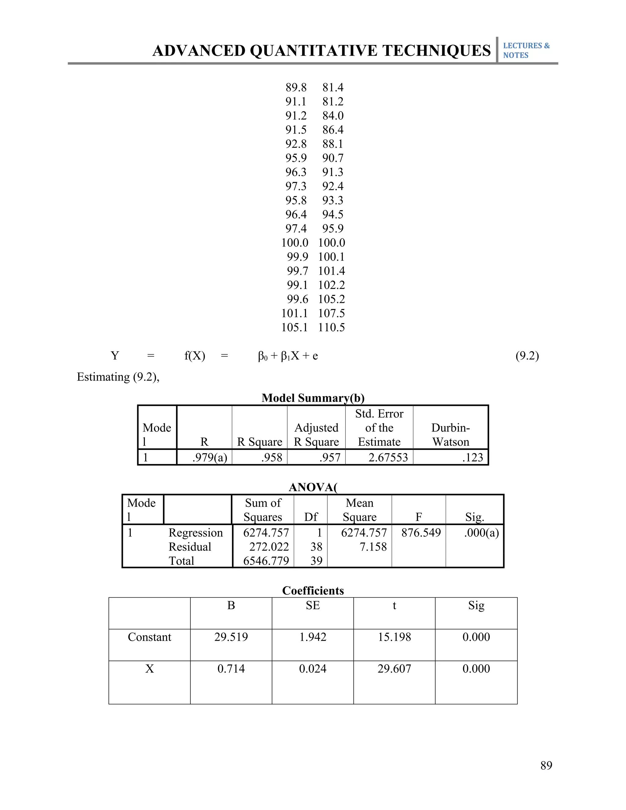
How to test? The estimated model (9.2) estimates DW = 0.123, which needs to compare with
the tabulated values provided in the Durban-Watson d statistic tables. We have n = 40 and K’ = 1
(k excluding intercept). At n = 40 and K’= 1, table provides dl = 1.442 and du = 1.544. As
calculated DW = 0.123 falls below du, that suggests existence of the problem of autocorrelation.

Remedies (Gujarati 2007, pages 485-495)
There are two major remedies, namely:
(a) When the ‘coefficient of autocorrelation’ (rho = ρ) is not known, then remedy is
‘first-differencing’, that is:
(Yt – Yt-1) = β1(Xt – Xt-1) + et (9.6a)
(b) When ρ is known, then remedy is:
(Yt – ρYt-1) = α + β1(Xt – ρXt-1) + et (9.6b)
The First-Differencing method
Using TRANSFORM and COMPUTE command in SPSS, we can generate lagged variables,
namely:
LagY = Yt-1
LagX = Xt-1
Further generating FDY = Yt – Yt-1 = Yt – LagY (9.7a)
and FDX = X = Xt-1 = Xt – LagX (9.7b)

95

LECTURES &

Running regression:
FDY = α + β1FDX + et (9.8)
Results are:

Model Summaryc,d

Adjusted R Std. Error of the
b
Model R R Square Square Estimate Durbin-Watson

1 .831a .690 .683 .92580 1.611

a. Predictors: FDX

b. For regression through the origin (the no-intercept model), R Square measures the
proportion of the variability in the dependent variable about the origin explained by
regression. This CANNOT be compared to R Square for models which include an intercept.

c. Dependent Variable: FDY

d. Linear Regression through the Origin

Residuals Statisticsa,b

Minimum Maximum Mean Std. Deviation N

Predicted Value -2.9518 .6480 -1.1393 .76208 40

Residual -1.84013 2.14796 -.02567 .92543 40

Std. Predicted Value -2.378 2.345 .000 1.000 40

Std. Residual -1.988 2.320 -.028 1.000 40

a. Dependent Variable: FDY

b. Linear Regression through the Origin

Coefficientsa,b

Standardized
Unstandardized Coefficients Coefficients

Model B Std. Error Beta t Sig.

1 FDX .720 .077 .831 9.328 .000

a. Dependent Variable: FDY

b. Linear Regression through the Origin

The results have improved, especially in terms of DW statistic, which is now = 1.611.
Since no-autocorrelation zone ranges between du and 4-du, that is:
du = 1.544 and 4 – du = 4 – 1.544 = 2.456

96

LECTURES &

The calculated DW = 1.611 falls within the no-autocorrelation zone, suggesting that there exists
no autocorrelation problem, now.

The Rho-Corrected regression
Where the ‘coefficient of autocorrelation’ (rho = ρ) is known, or can be estimated, the value of
the ρ is used for correction of autocorrelation in the following form.
(Yt – ρYt-1) = α + β1(Xt – ρXt-1) + et (9.9)
The coefficient of autocorrelation ρ (rho) can be calculated, using the estimated DW statistic, as
follows.
DW = d = 2(1 – ρ) (9.10a)
ρ = 1 – (d/2) (9.10b)
In our original model (9.2), DW estimates at 0.123; putting this value in 9.10b:
ρ = 1 – (d/2) (9.11a)
= 1 – (0.123/2)
= 1 – 0.0615
= 0.9385 (9.11b)
Substituting ρ = 0.9385 in (9.9),
(Yt – 0.9385Yt-1) = α + β1(Xt – 0.9385Xt-1) + et (9.12)
and running the regression.

Prais-Winsten transformation: In case of the use of both cases of the First-differencing or the
Rho-Corrected regression, the first observation, because of not having any antecedent is lost; in
such situation, Prais-Winsten transformation helps to make good of this loss. According to this
transformation, the first observation can be retained after transforming it in the following way.
Y1 √(1 – ρ2) and Y1√(1 – ρ2) (9.13)
The correction of Autocorrelation through the use of First-differencing or Rho-corrected
regression is referred generally referred to as Generalized Least Square (GLS); when instead o
true ρ, estimated ρ is used, the method is known as Feasible GLS (FGLS) or Estimated GLS
(EGLS). In case, GLS is used with Prais-Winsten transformation, method is then called Full
EGLS or FEGLS (Gujarati 2007, pp.487-494).

97

LECTURES &

The Heteroscadasticity-and-autocorrelation consistent standard errors (HAC)
Instead of using the FGLS methods discussed earlier, one can use OLS after correcting standard
errors for autocorrelation the procedure developed by Newey and West 15 This method is an
extension of White’s heteroscedasticity-consistent standard errors discussed earlier under
Heteroscadasticilty. The corrected standard errors are known as HAC (heteroscedasticity- and
autocorrelation-consistent) standard errors or simply as Newey–West standard errors. Most
modern computer packages now calculate the Newey–West standard errors. However, it is
important to point out that the Newey–West procedure is strictly speaking valid in large samples
and may not be appropriate in small samples. Therefore, if a sample is reasonably large, one
should use the Newey–West procedure to correct OLS standard errors not only in situations of
autocorrelation only but also in cases of heteroscedasticity, for the HAC method can handle both,
unlike the White method, which was designed specifically for heteroscedasticity (Gujarati 2007,
pp.494-95)

OLS versus FGLS and HAC
In the presence of autocorrelation, OLS estimators, although unbiased, consistent, and
asymptotically normally distributed, are not efficient. Therefore, the usual inference procedure
based on the t, F, and χ2 tests is no longer appropriate. On the other hand, FGLS and HAC
produce estimators that are efficient, but the finite, or small-sample, properties of these
estimators are not well documented. This means in small samples the FGLS and HAC might
actually do worse than OLS. As a matter of fact, in a Monte Carlo study Griliches and
Rao46 found that if the sample is relatively small and the coefficient of autocorrelation,
ρ, is less than 0.3, OLS is as good or better than FGLS. As a practical matter, then, one may use
OLS in small samples in which the estimated Rho is, say, less than 0.3 (Gujarati 2007, p,495).

15
W. K. Newey, and K. West, “A Simple Positive Semi-Definite Heteroscedasticity and Autocorrelation
Consistent Covariance Matrix, Econometrica, vol. 55, 1987, pp. 703–708.

98

LECTURES &

TOPICS 10 – 15
SPECIAL APPLICATIONS

Topic 10
Mediation analysis: problems and prospects

Topic 11
Moderation analysis: problems and prospects

Topics 12 - 13
Time-series analysis: problems and prospects

Topic 14
Panel data analysis: problems and prospects

Topic 15
Minimization, maximization and optimization

Topic 16
Welfare analysis: maximization of producer and consumer
surpluses and minimization of social costs

99

Aqt instructor-notes-final

More Related Content

Similar to Aqt instructor-notes-final

Aqt instructor-notes-final