This document discusses analytical models of learning curves with variable processing times. It introduces the concept of learning curves where operators get faster at tasks over time. It presents the basic log-linear model used to mathematically represent learning curves. The objectives are to calculate processing times for single-machine and two-machine systems using different models that account for variability in processing times, like exponential and hypo-exponential distributions. Equations are developed and examples are shown for determining average and variability of processing times. Further work is identified to extend the calculations to two-machine systems with both infinite and finite buffer sizes.

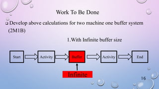
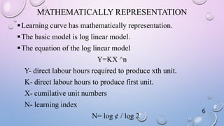
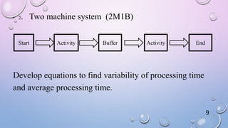
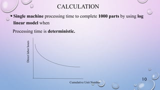
1. ANALYTICAL MODELS OF
LEARNING CURVES WITH
VARIABLE
PROCESSING TIME
M.S.P,MUTHUKUMARANAGE
E/11/267 1

2. New
labour
INTRODUCTION
2

3. INTRODUCTION
New or unskilled operators cannot achieved
acceptable speed at first time.
The operator will require less and less time to
complete the similar task as time goes on.
This is the basic concept of learning curves.
3

4. INTRODUCTION
The concept of learning curve was
reported by wright in 1936.
Wright developed a mathematically
representation of learning curve
4

5. LEARNING RATE (¢)
 The operator’s performance will improve at a constant rate each time
the output doubles.
5

6. MATHEMATICALLY REPRESENTATION
Learning curve has mathematically representation.
The basic model is log linear model.
The equation of the log linear model
Y=KX ^n
Y- direct labour hours required to produce xth unit.
K- direct labour hours to produce first unit.
X- cumilative unit numbers
N- learning index
N= log ¢ / log 2
6

7. OTHER MODELS
1. The plateau model
2. The stanford-b model
3. The dejong model
4. The S model
Above all models are the different form of log linear model.
1
2
3
4
Cumulative unit number
Directlabourhoursper
unit
7

8. OBJECTIVES
Calculate the time to complete a given batch of items exactly for
1. One machine system
Start Buffer Activity End
8

9. • 2. Two machine system (2M1B)
Develop equations to find variability of processing time
and average processing time.
Start Activity Buffer Activity End
9

10. CALCULATION
 Single machine processing time to complete 1000 parts by using log
linear model when
Processing time is deterministic.
Cumulative Unit Number
Directlaborhours
10

11. 11

12. Processing time has exponential distribution.
1 2 3 4 5
Cumulative Unit Number
Directlaborhours
K
K3n
K4
n K5n
K2
n
Mean = K*Xn
12

13. Exponential distribution
Mean=1/λ
Probability density function = λ 𝑒−λ 𝑥
Hypo-exponential distribution
𝑀𝑒𝑎𝑛 = 𝑖=1
𝑛
1/ λ(i)
𝑉𝑎𝑟𝑖𝑎𝑛𝑐𝑒 = 𝑖=1
𝑛
1/ λ(i)2
13

14. CALCULATION
Considering hypo exponential distribution
Mean time for produce 1000 parts =1587 hr
Variance =3062 hr
0.008
0.007
0.006
0.005
0.004
0.003
0.002
0.001
0.000
X
Density
1479
0.025
1695
0.025
1587
Distribution Plot
Normal, Mean=1587, StDev=55.33
14

15. Results Using Other Models
Model Name Equation Mean Variance
Stanford-B
model
Y(x)=Y1(X+B)-b
1559.857 2813.13
Dejong’s
model
Y(x)=Y1[M+(1-M)X-b]
2428.25 6336.51
15

16. Work To Be Done
 Develop above calculations for two machine one buffer system
(2M1B)
1.With Infinite buffer size
Start Activity Buffer Activity End
Infinite 16

17. 2. With finite buffer size(by increasing one by one)
Start Activity
Buffer
Size= 1
Activity End
Start Activity
Buffer
size=2
Activity End
17

18. THANK YOU
18