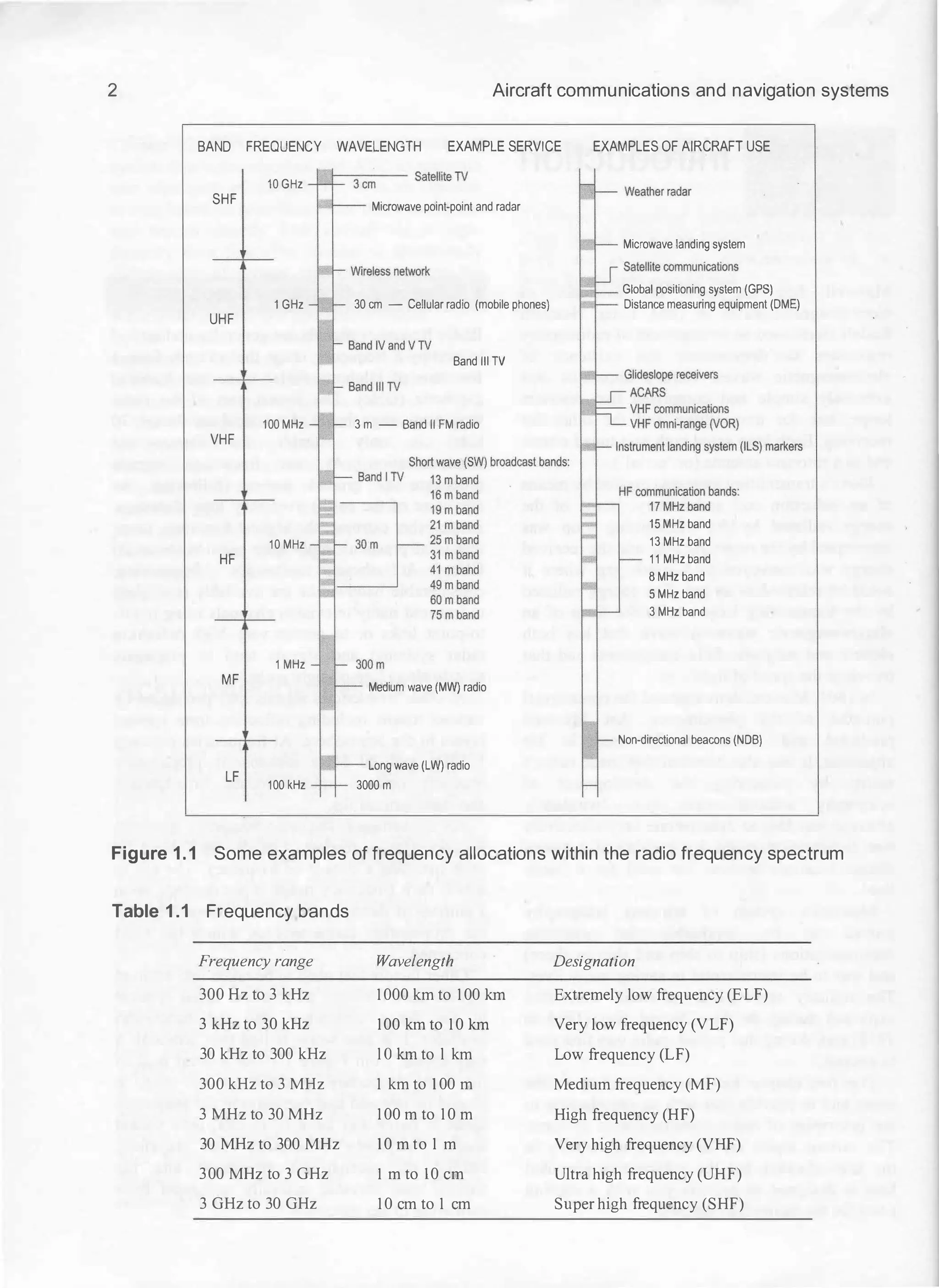
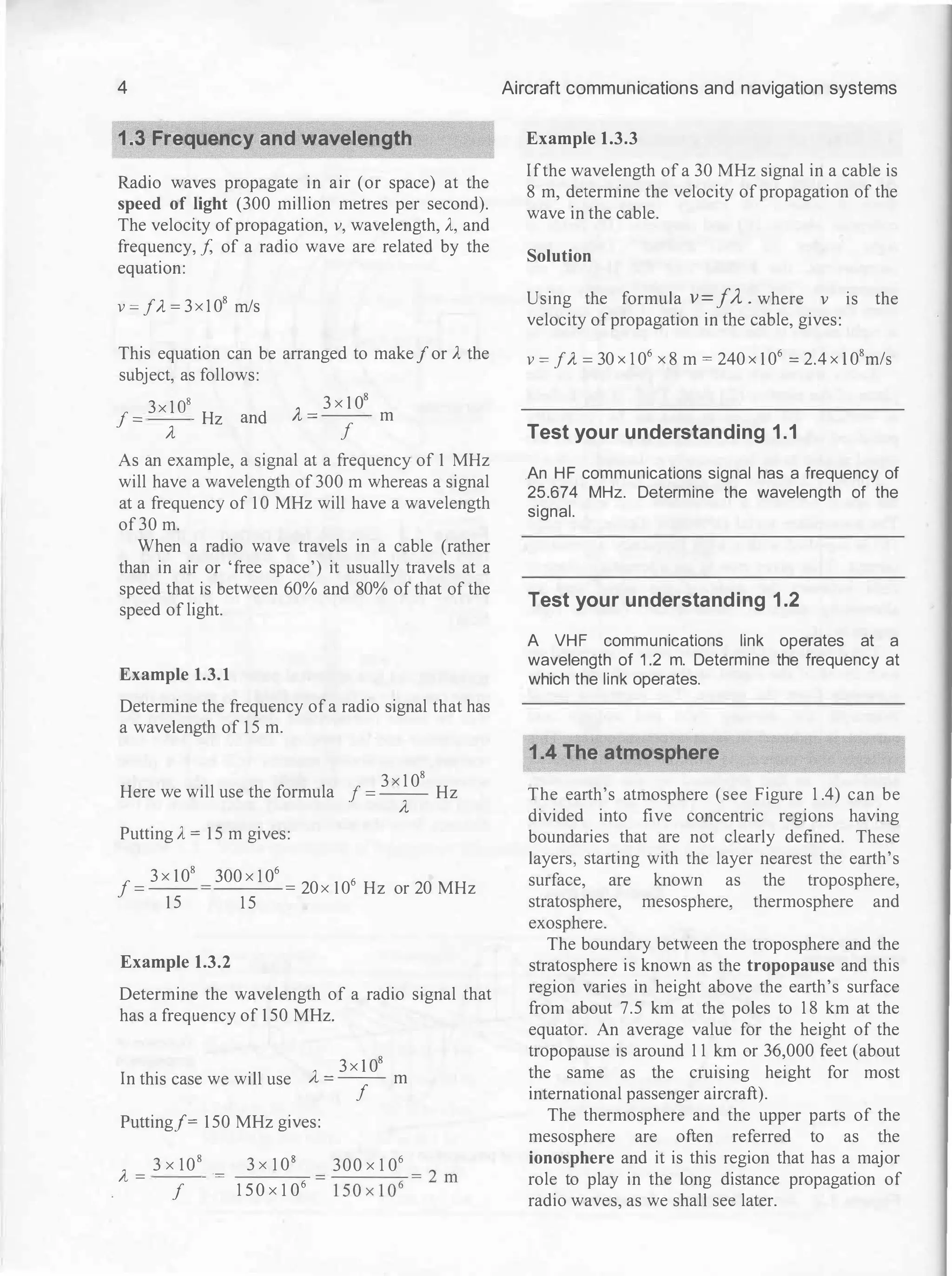
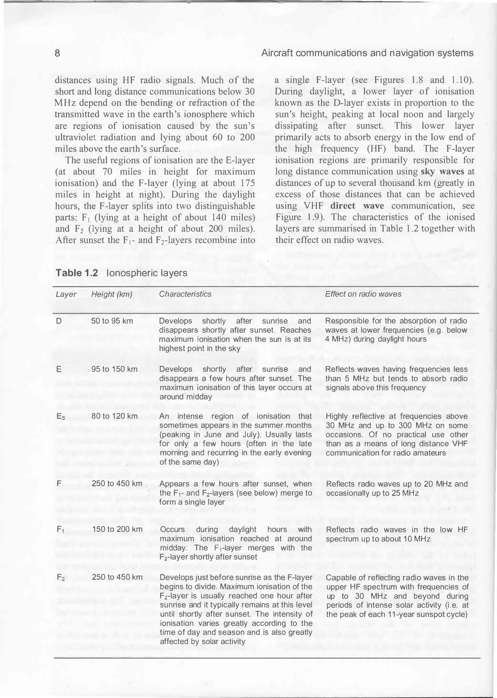
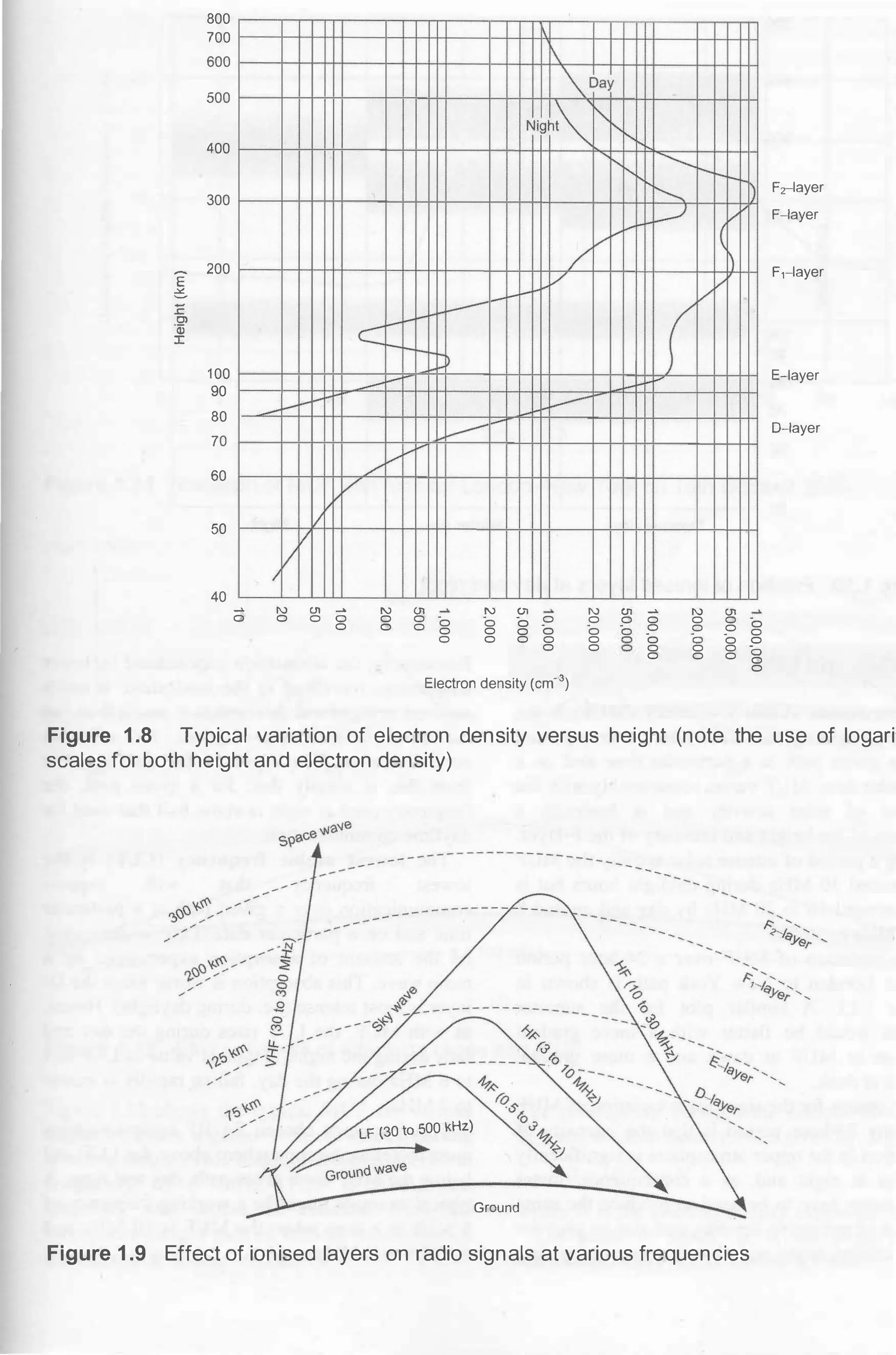
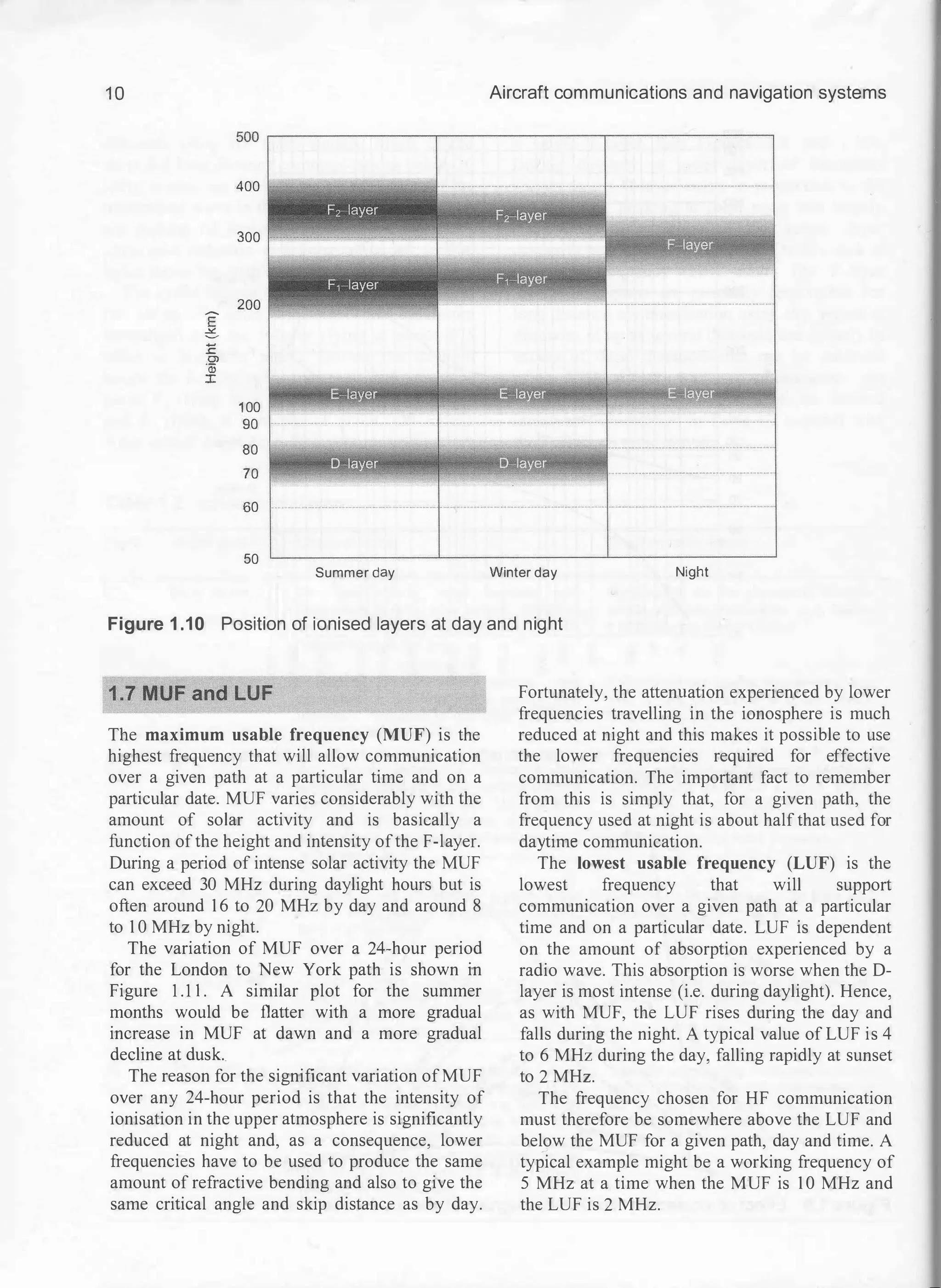
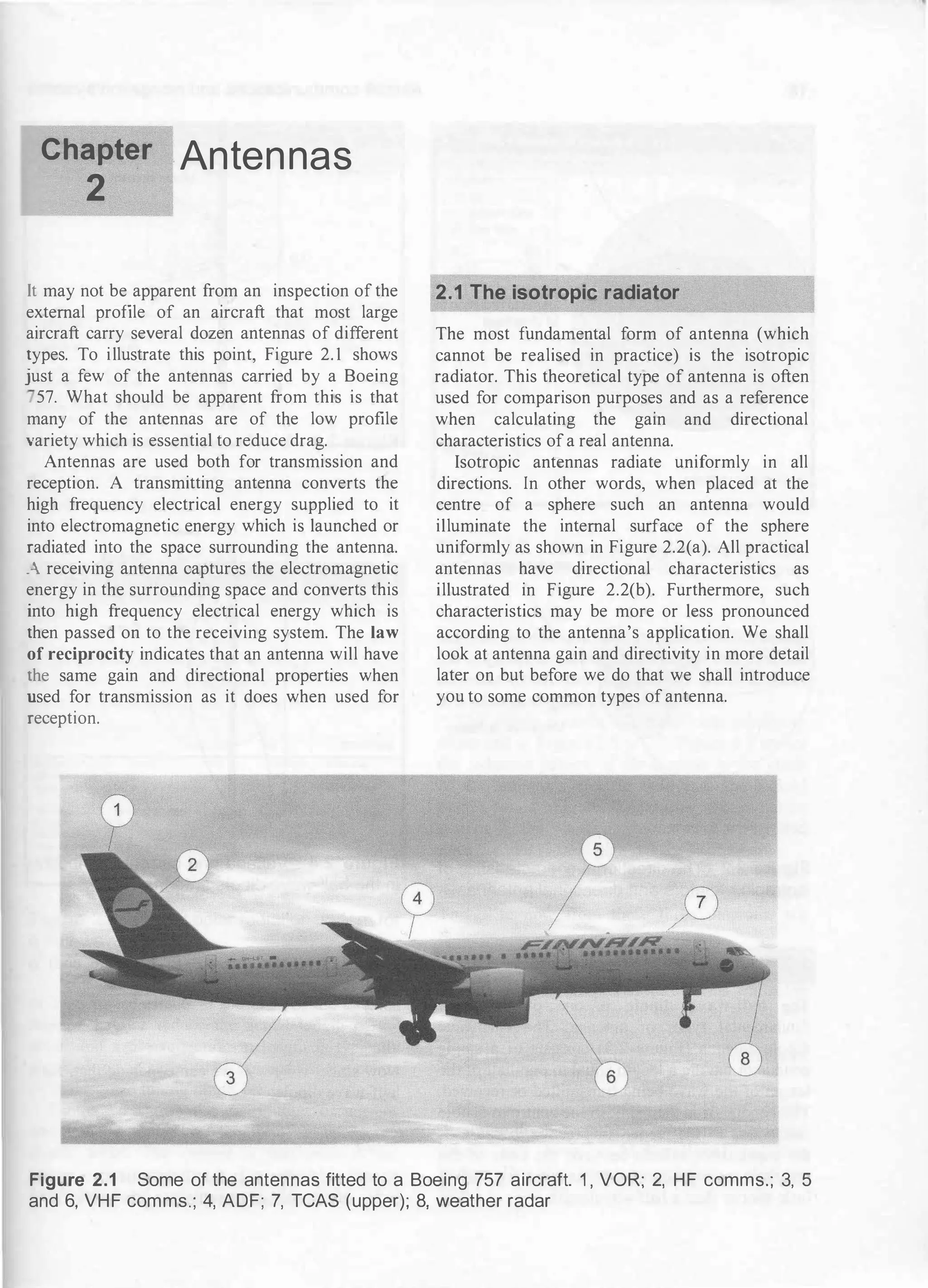
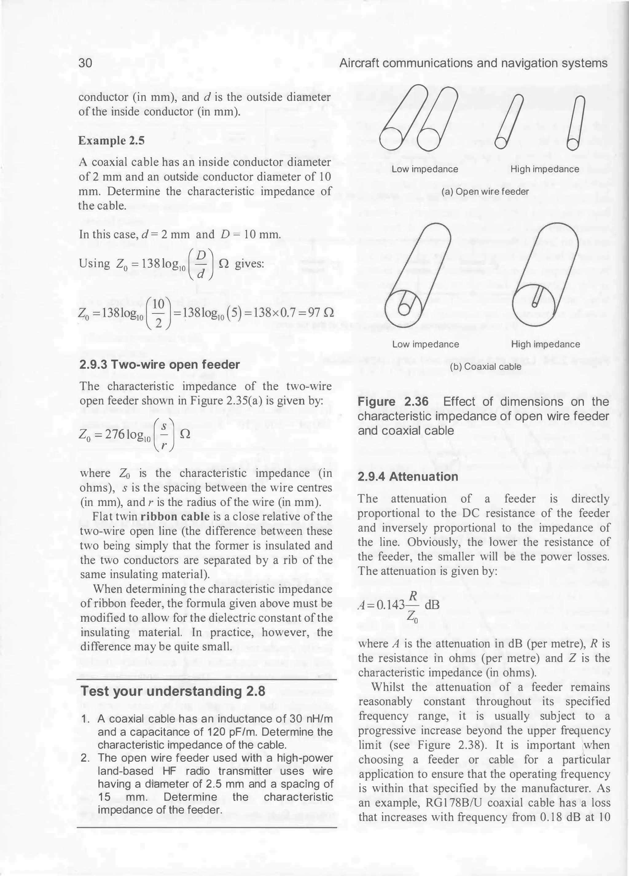
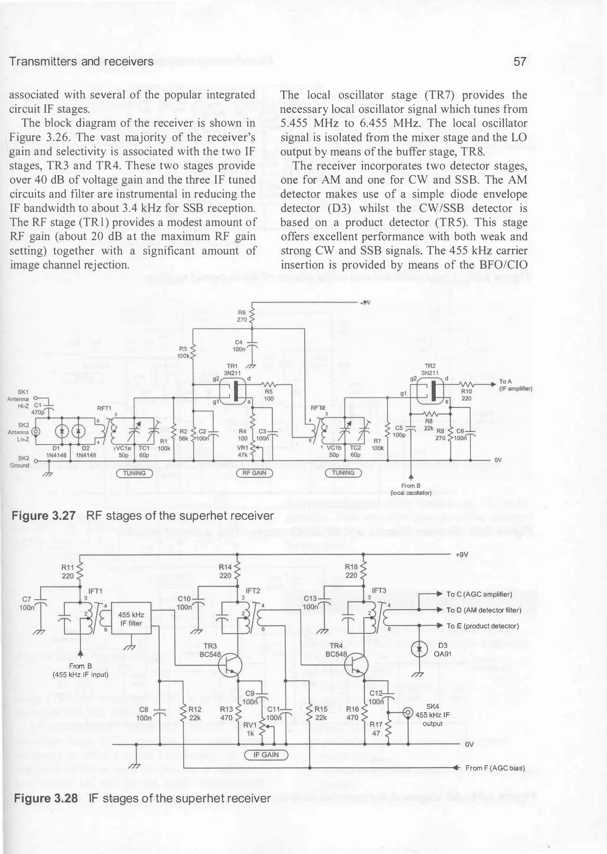
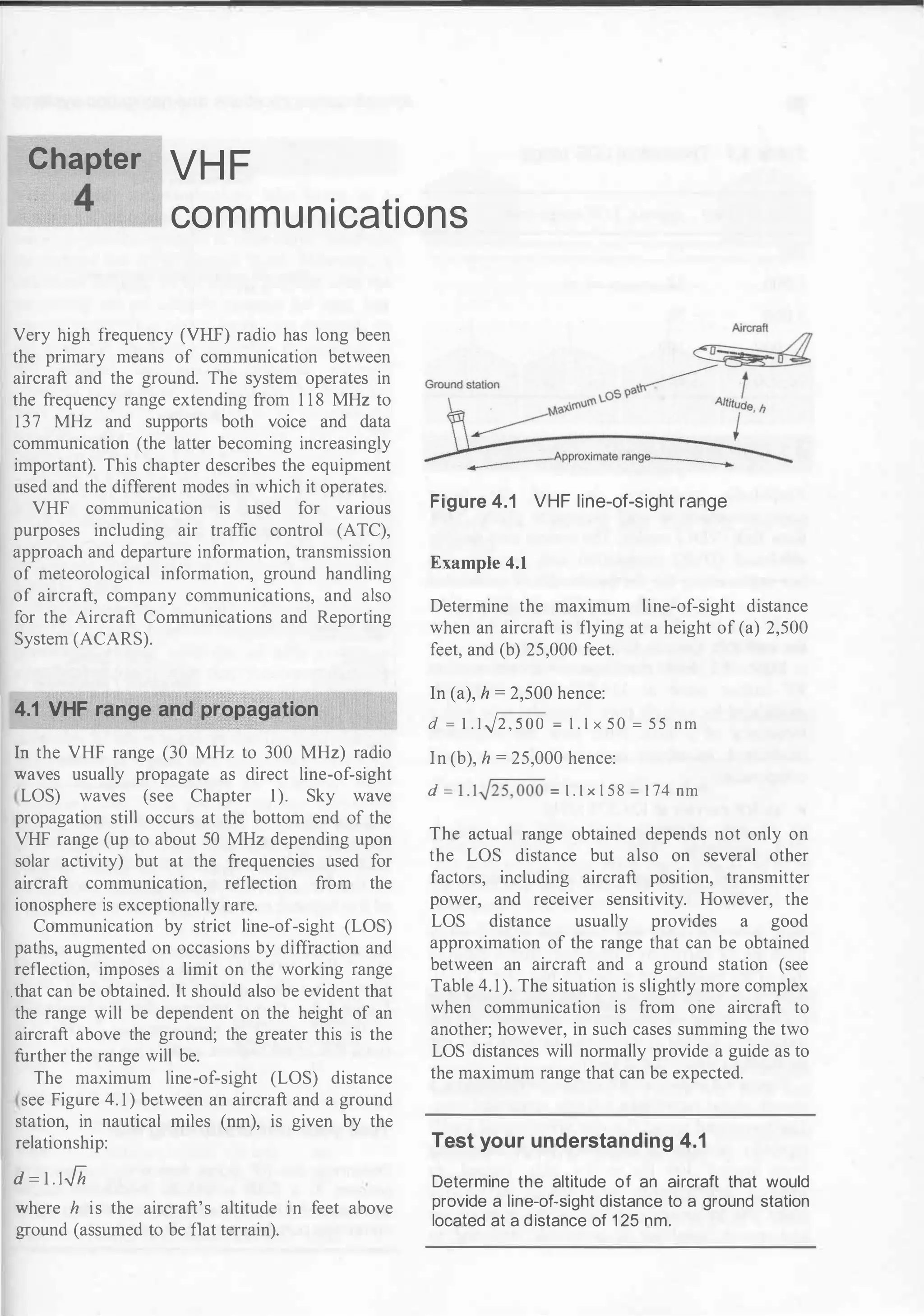
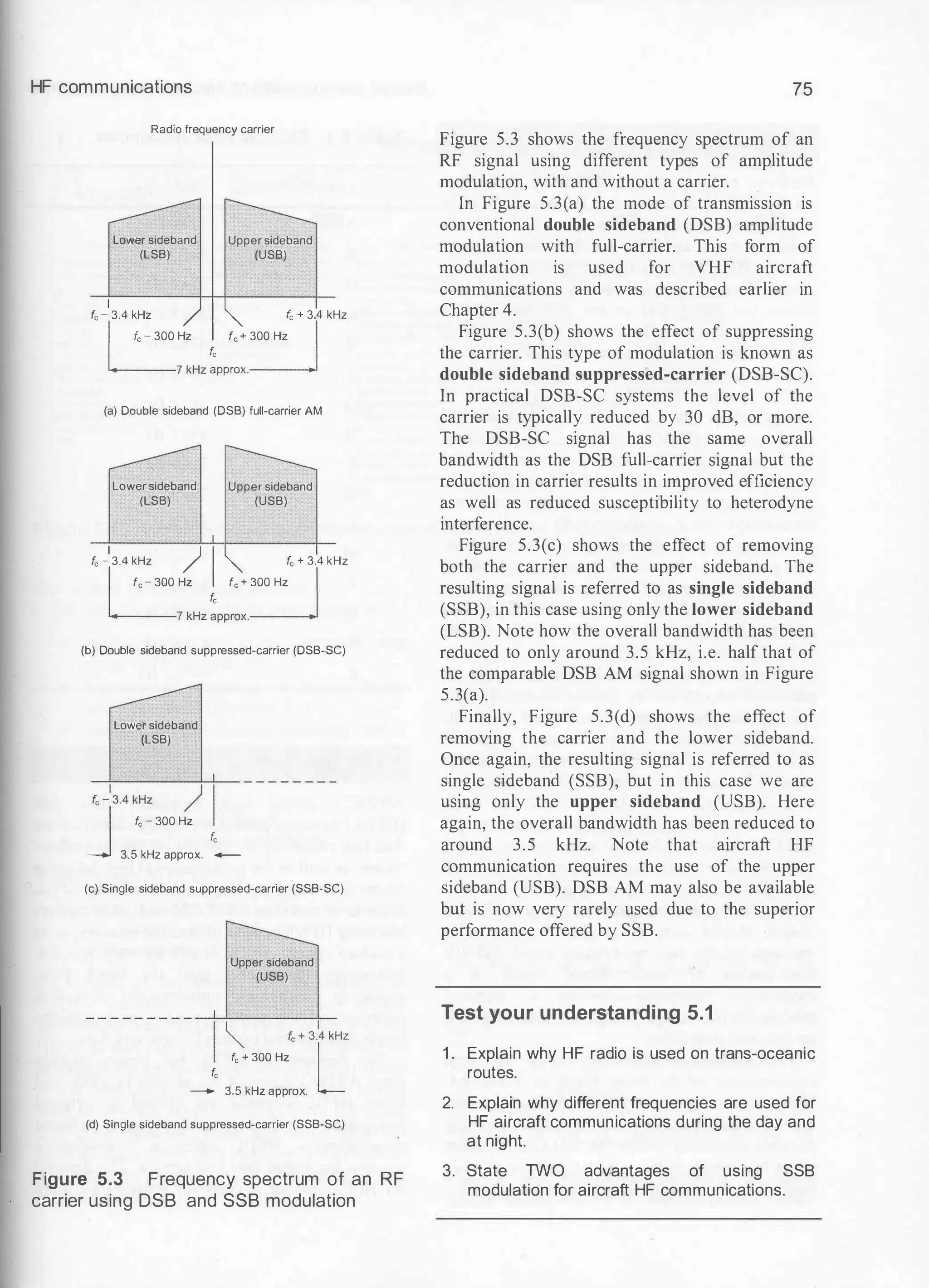
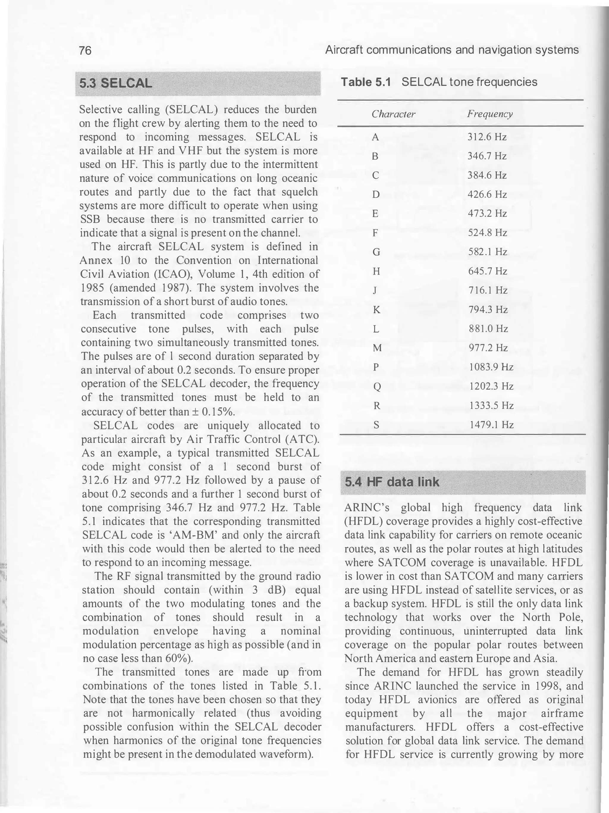
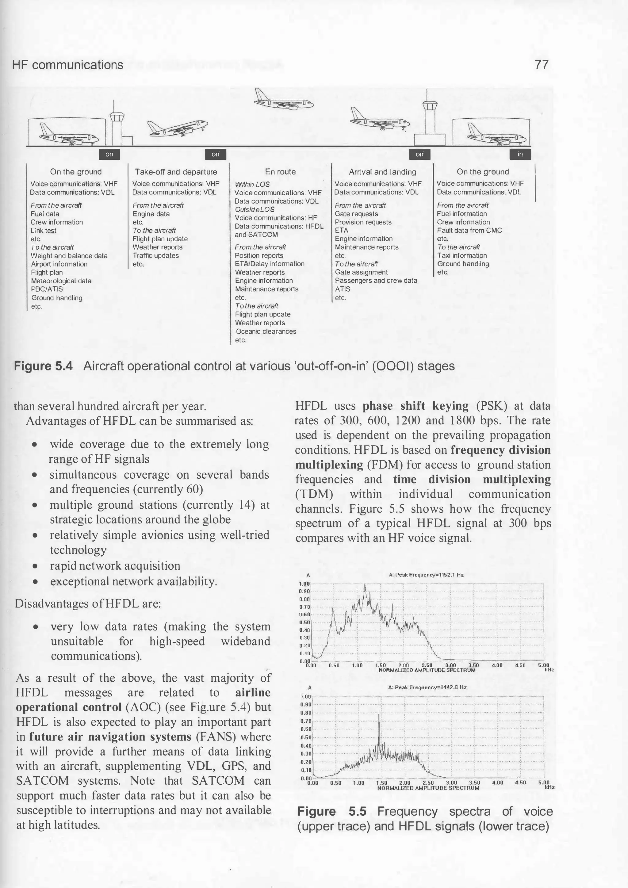
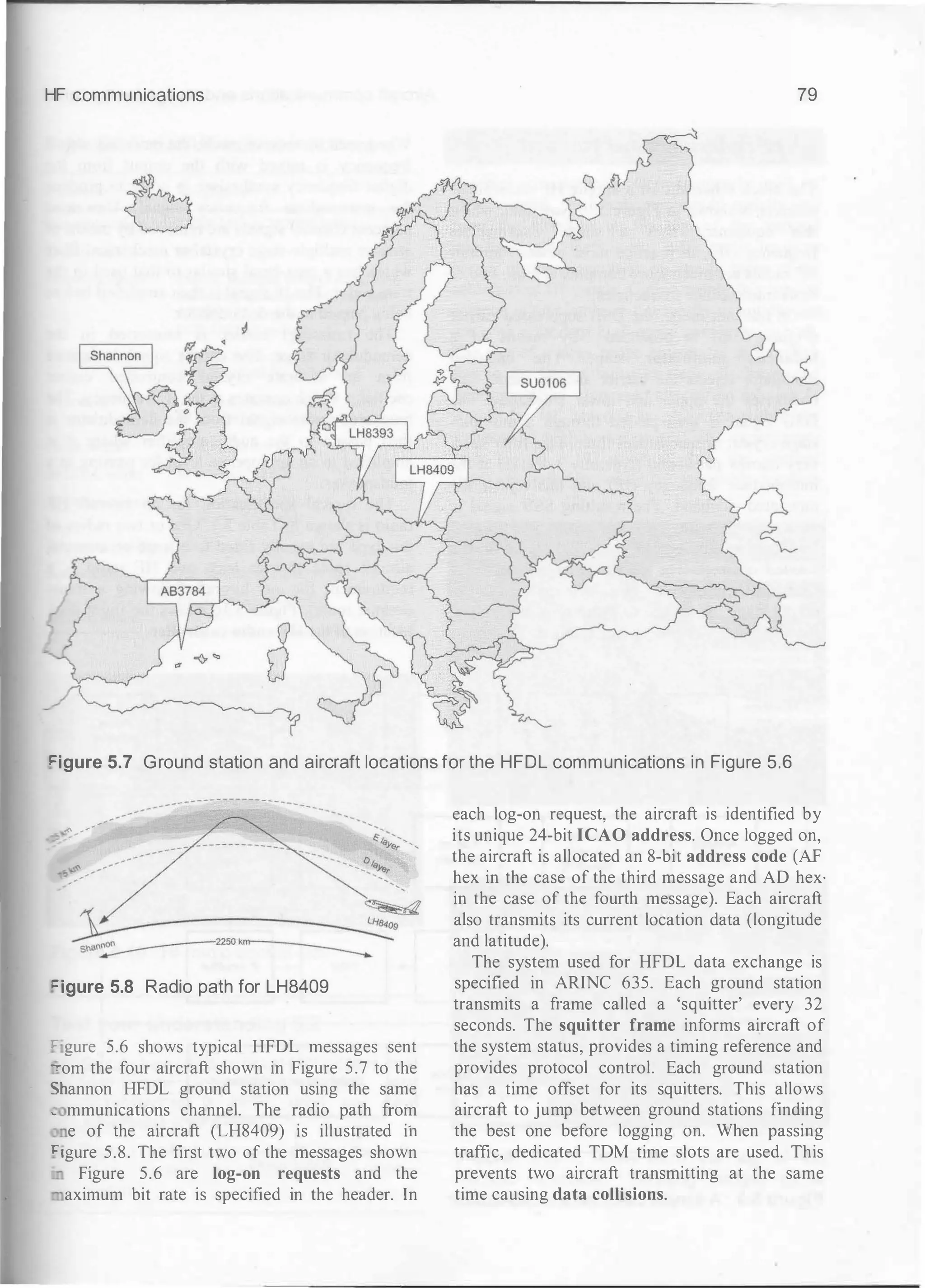
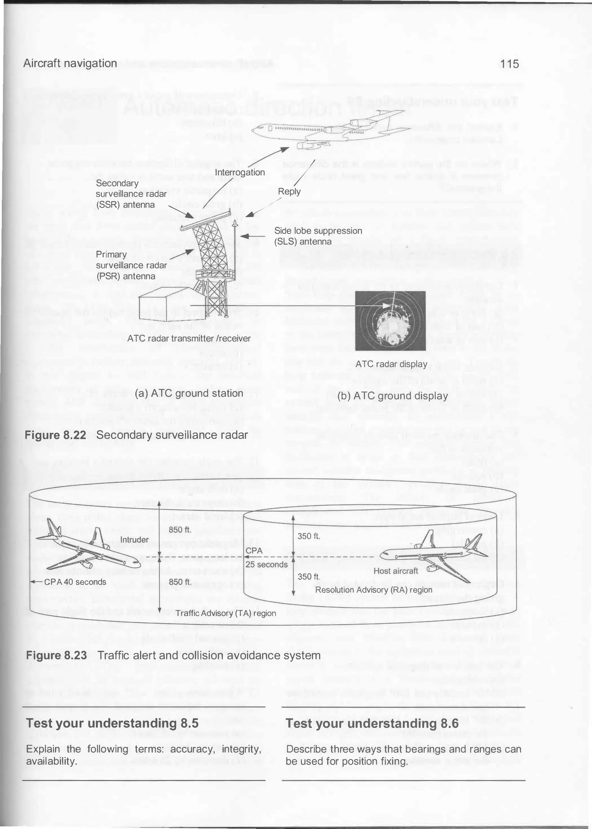
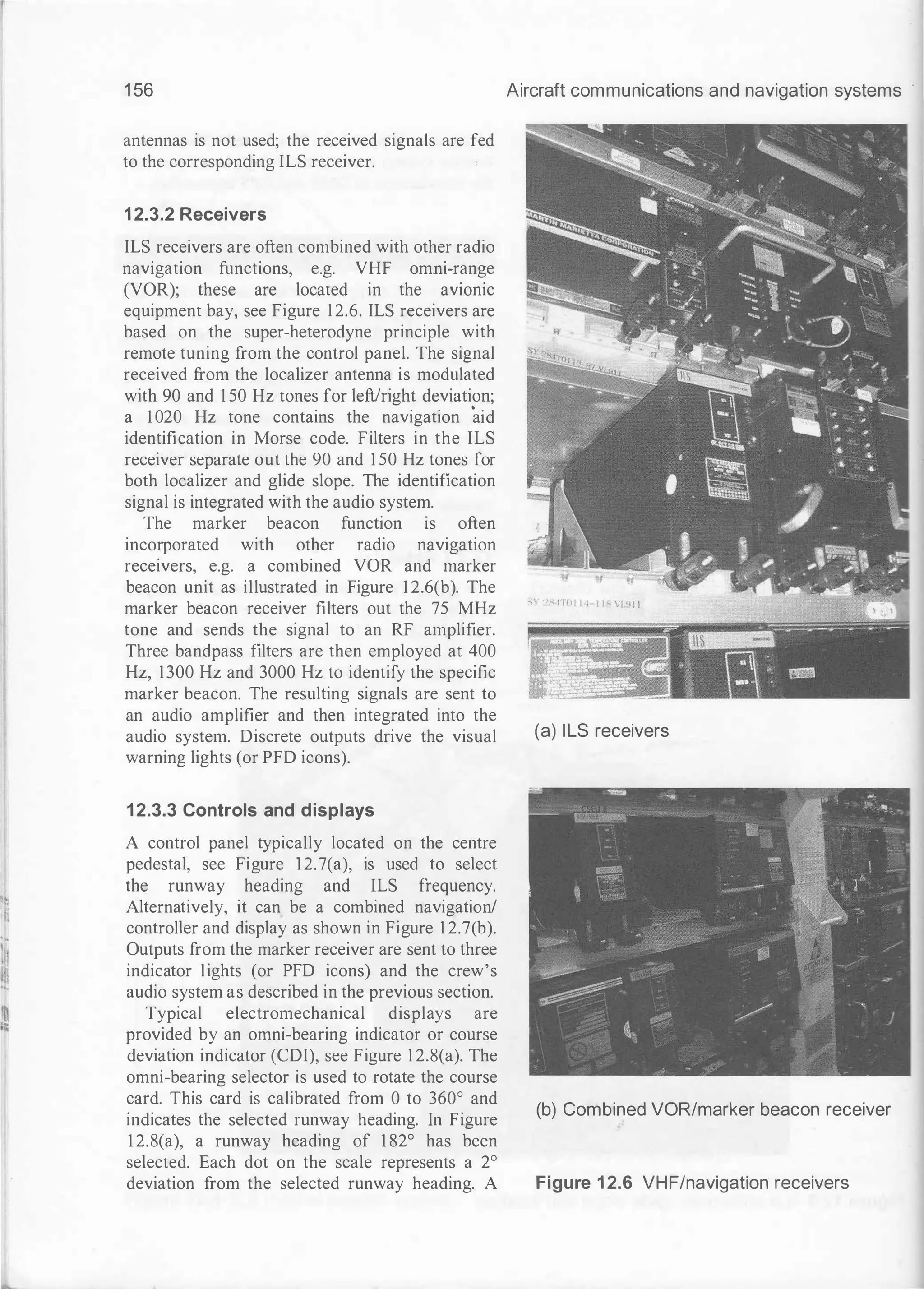
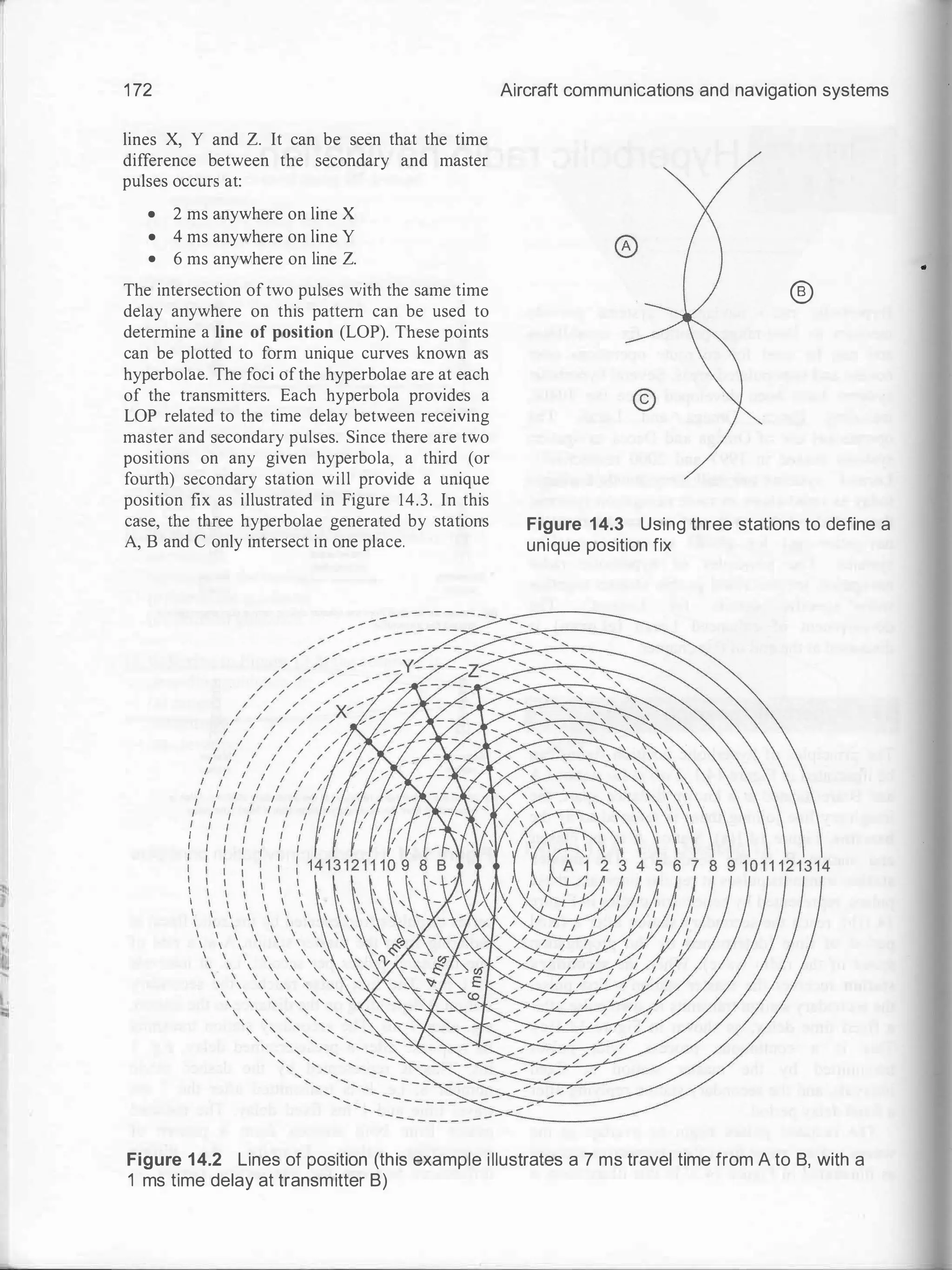
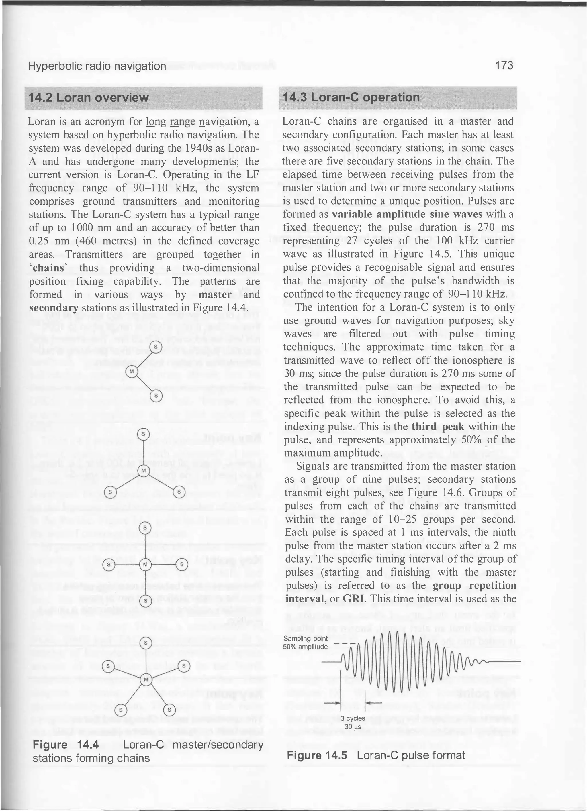
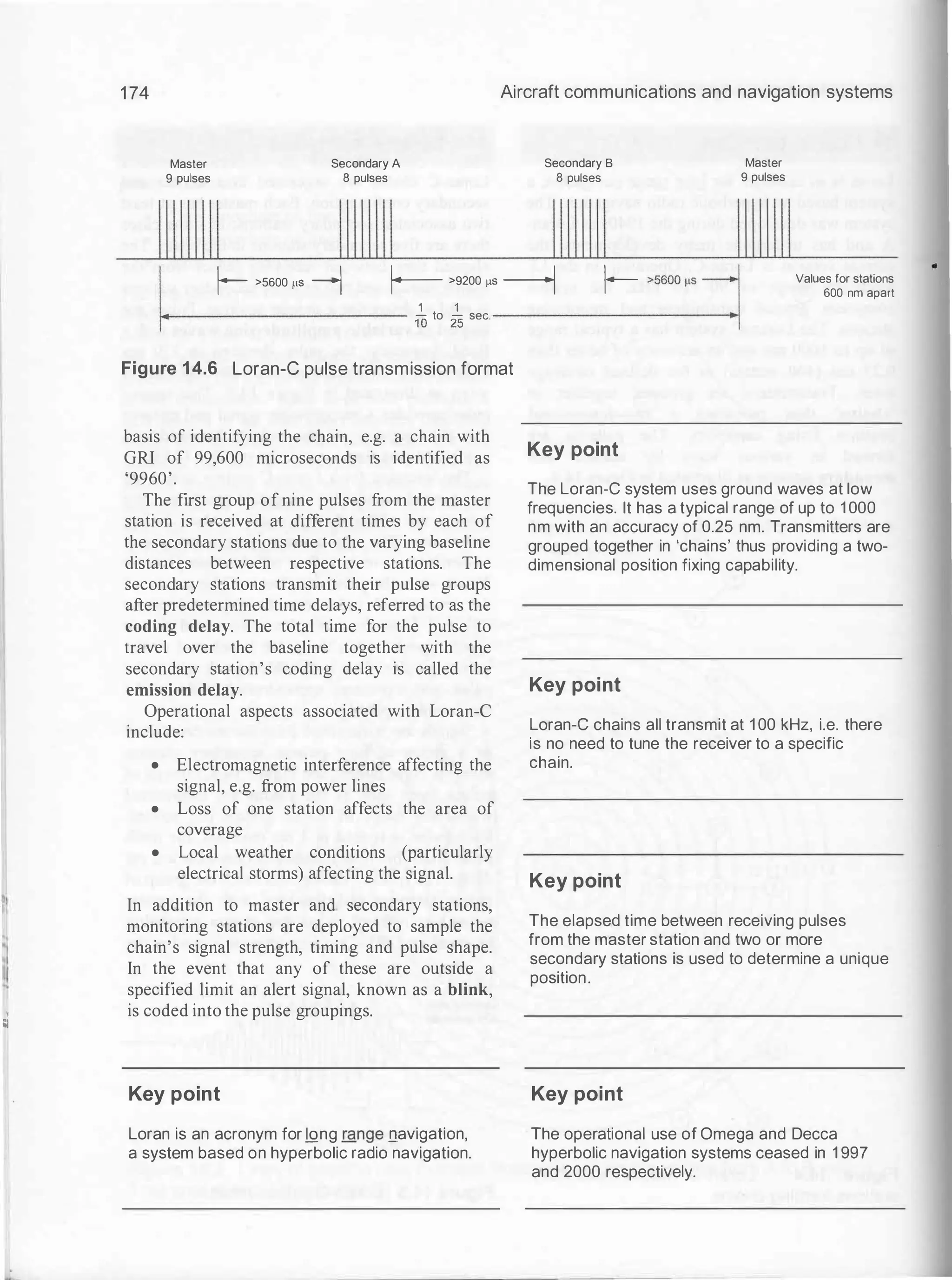
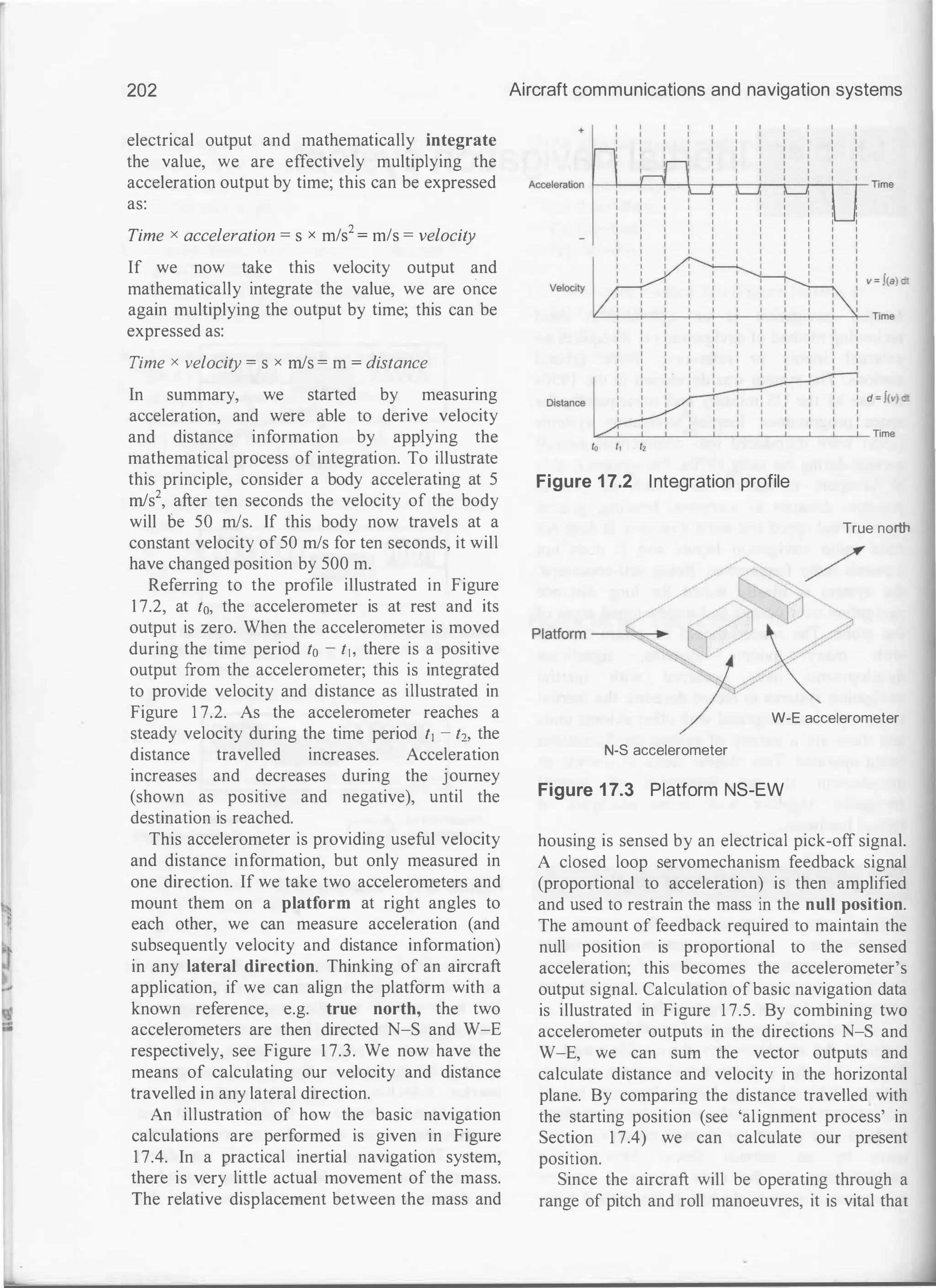
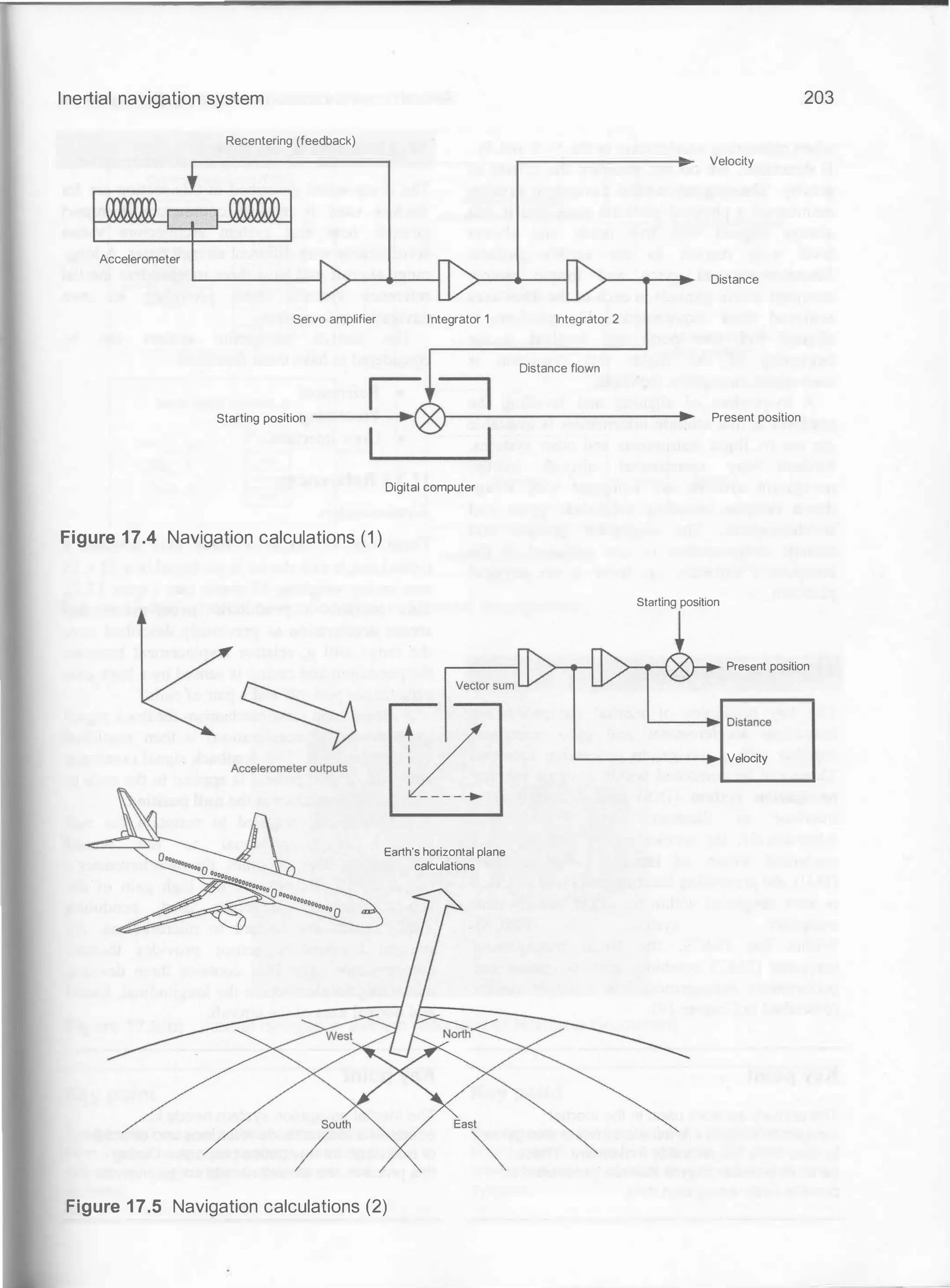
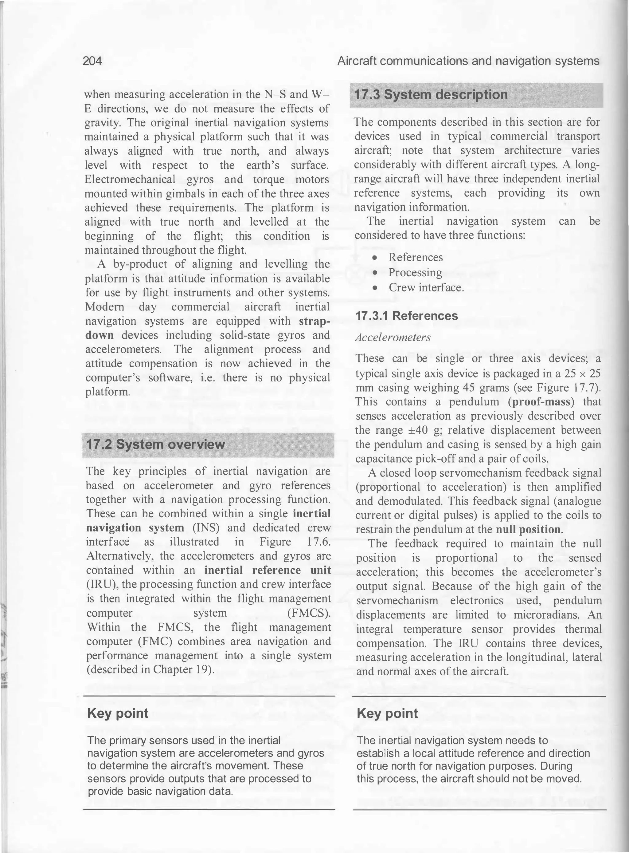
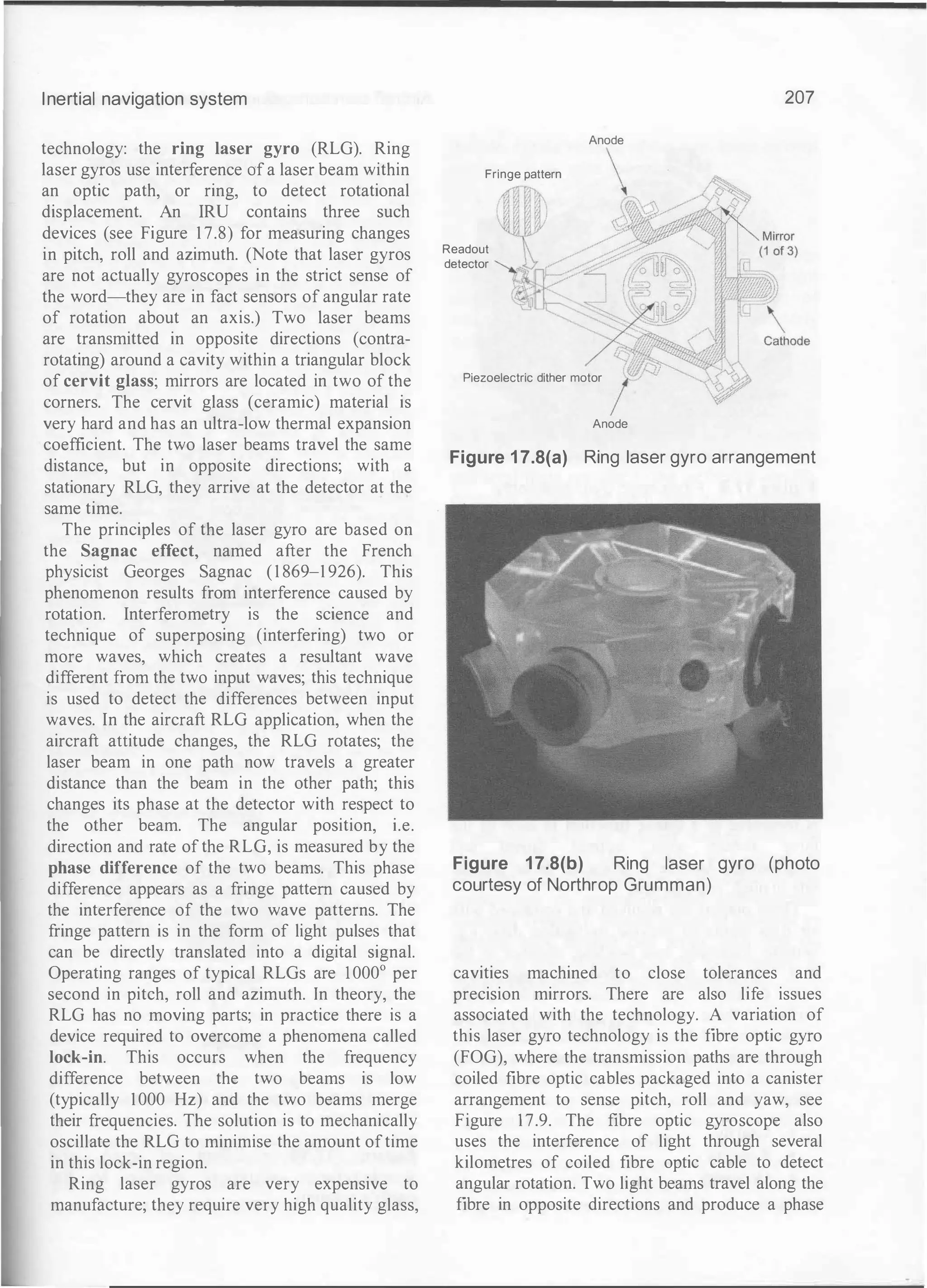
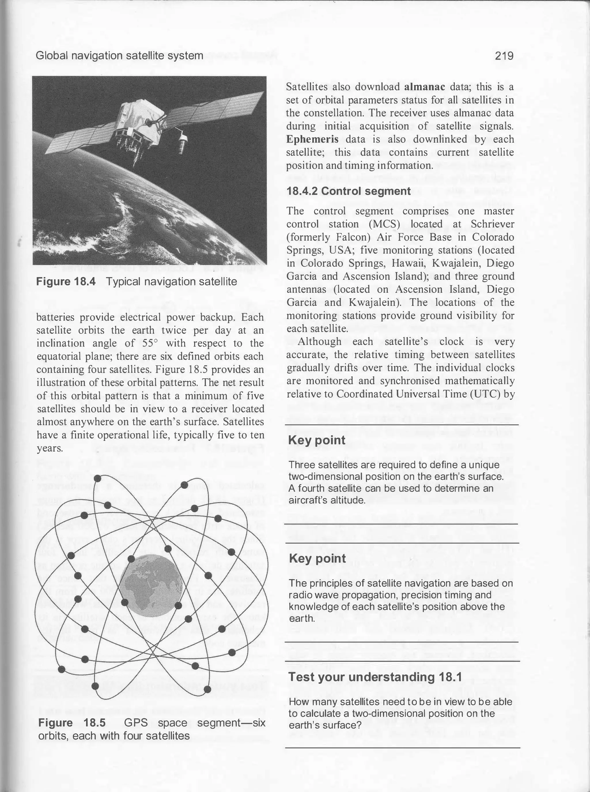
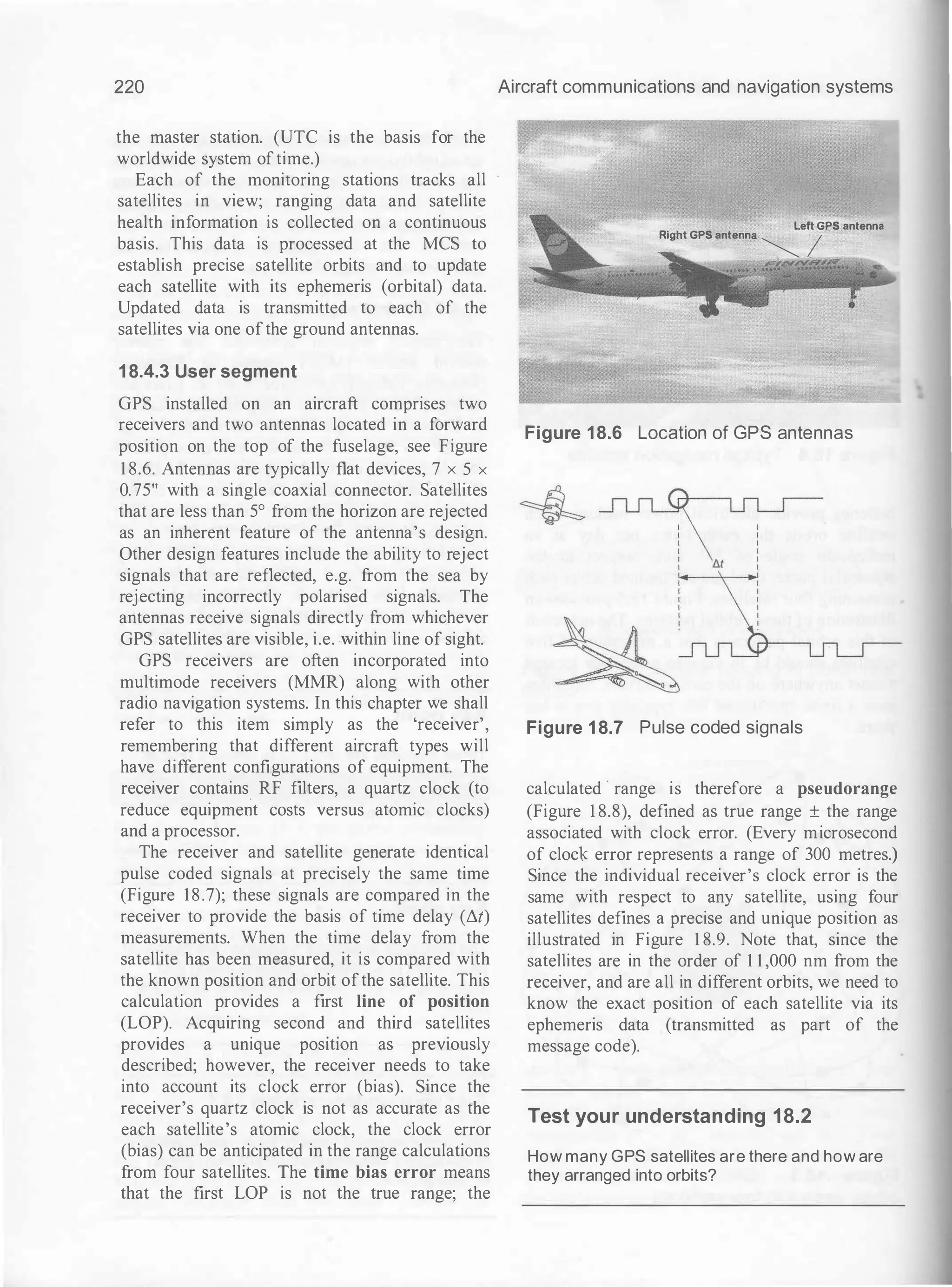
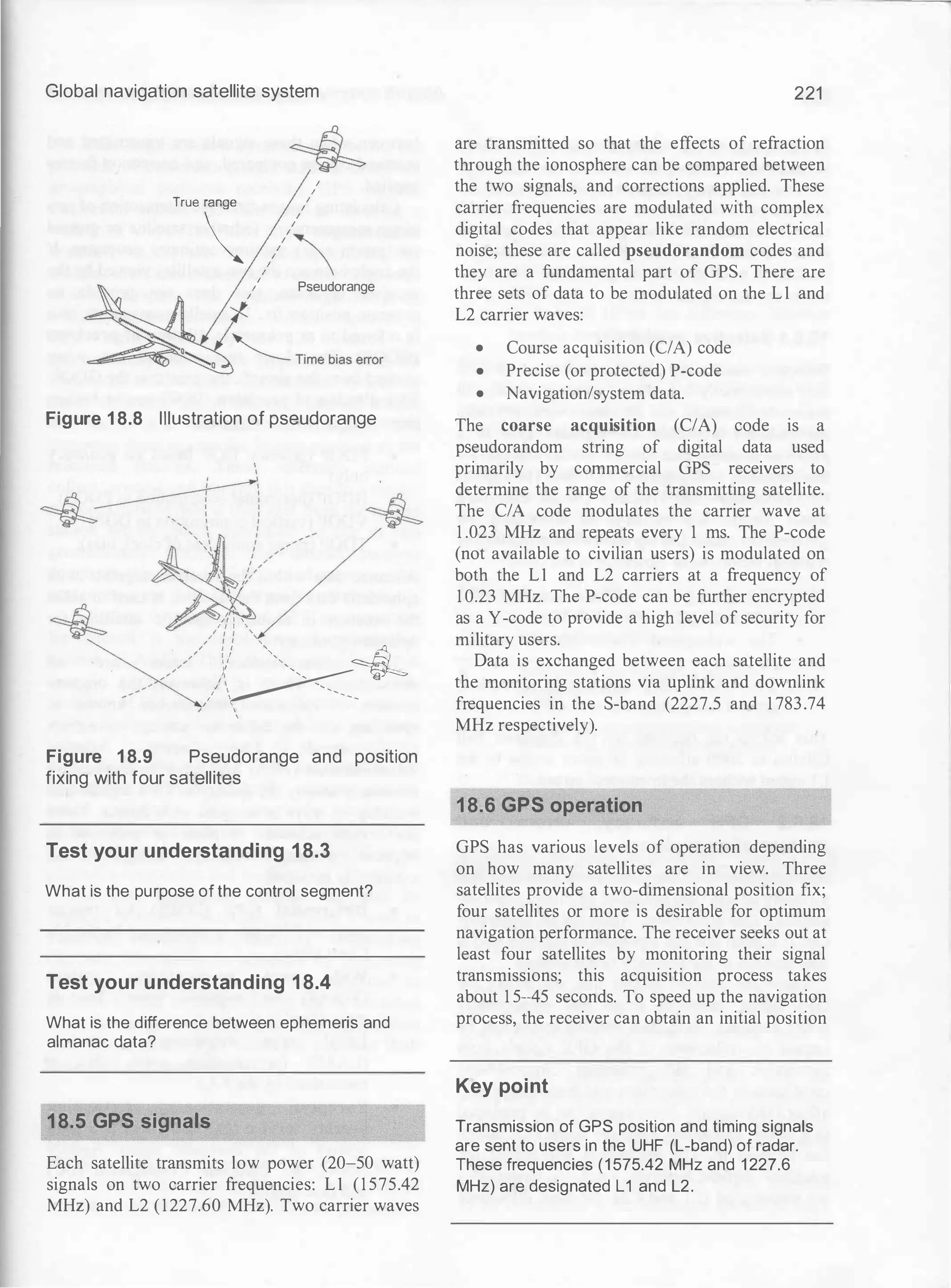
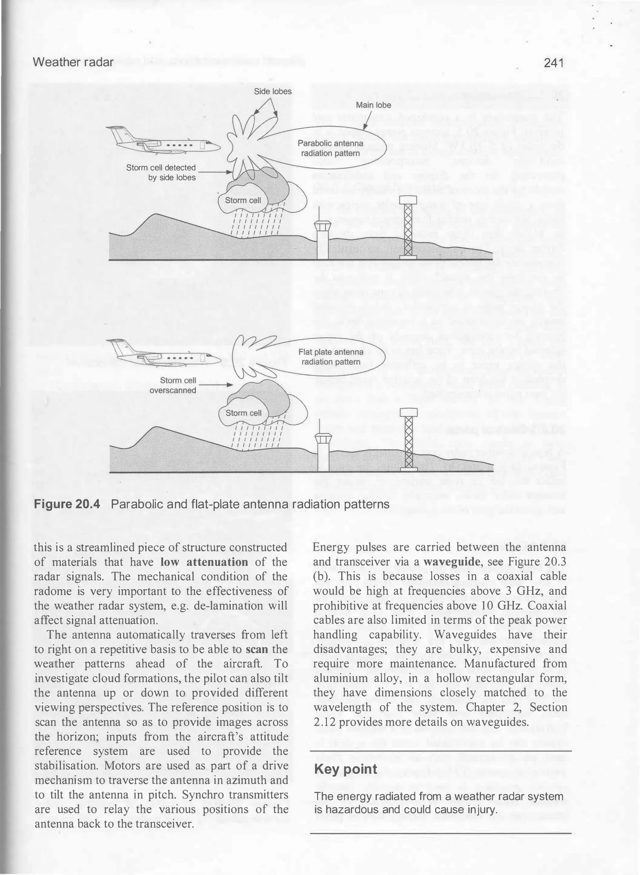
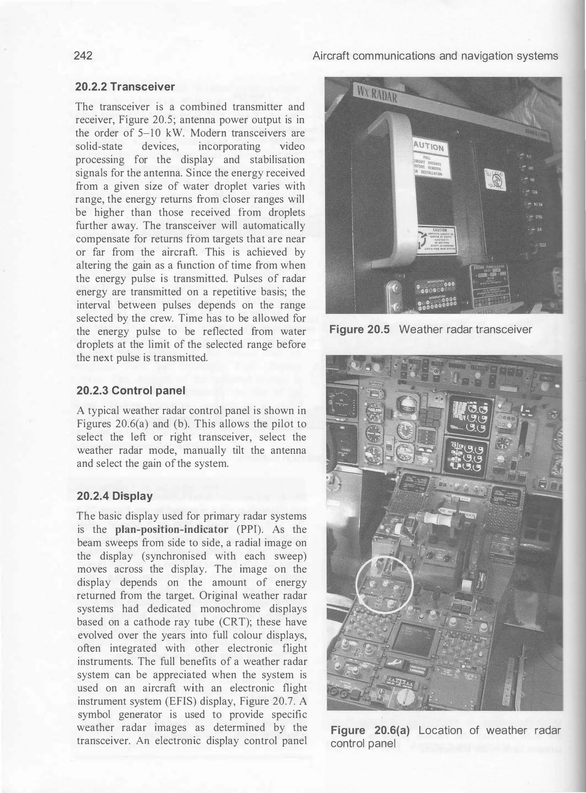
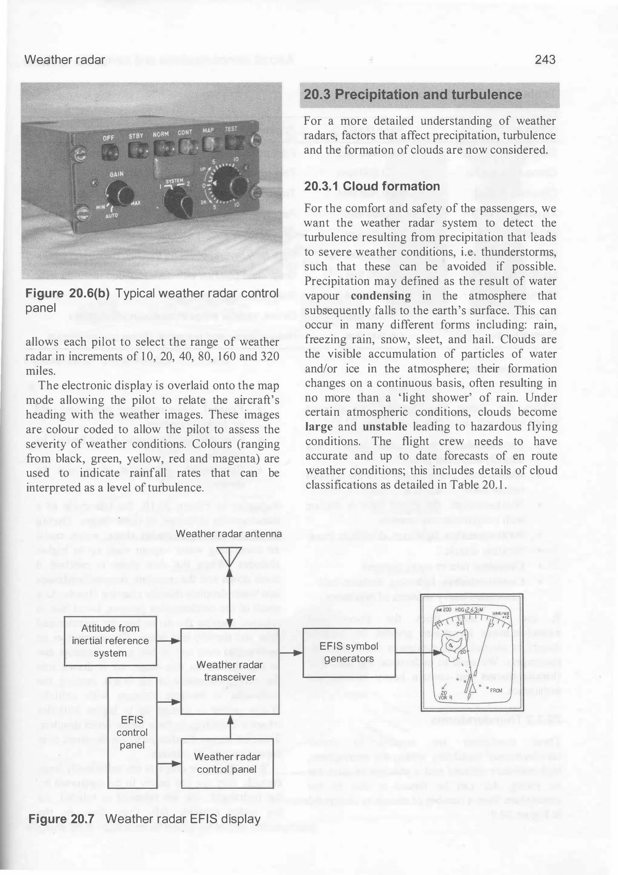
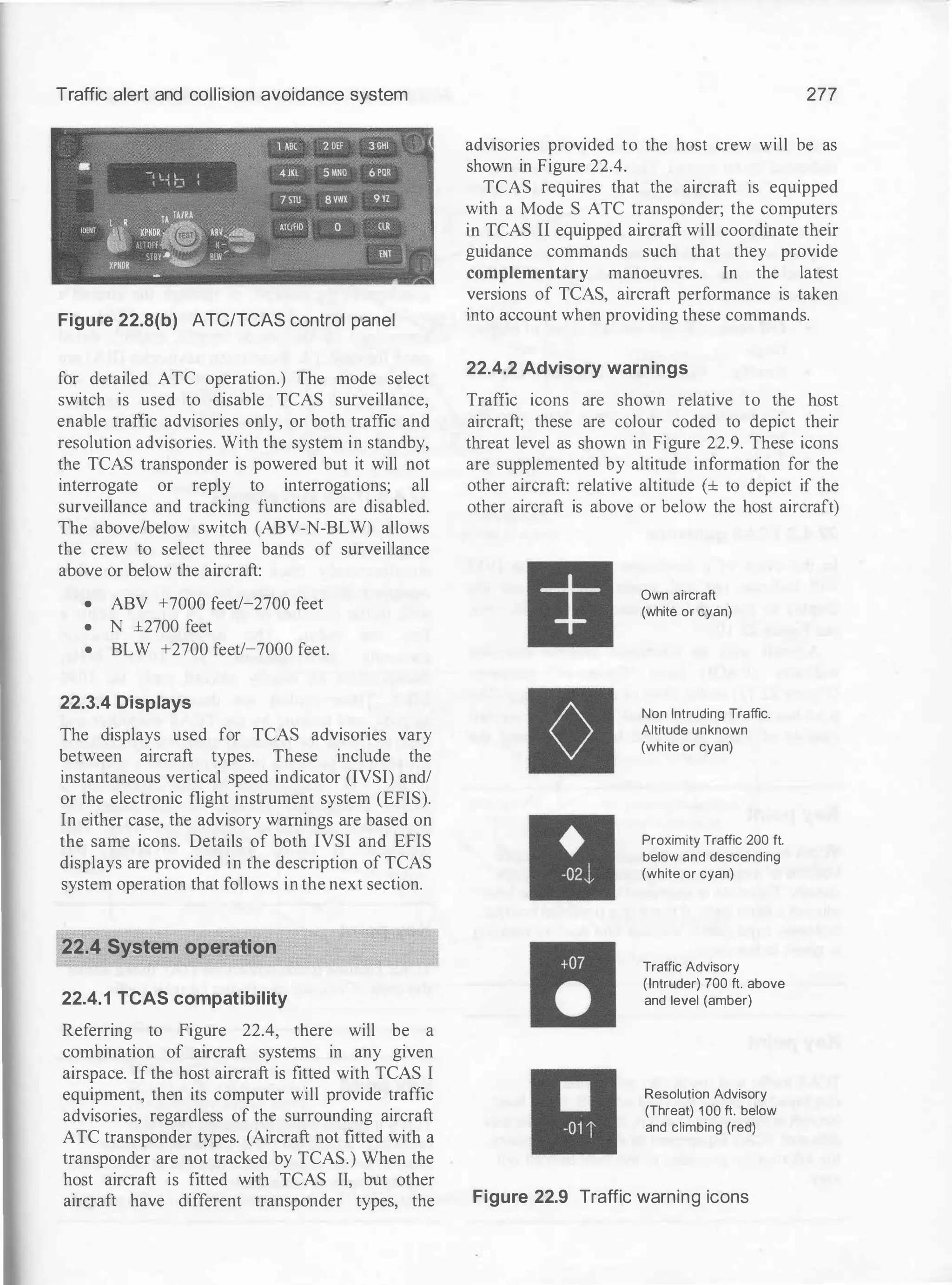
This document serves as a comprehensive guide to aircraft communications and navigation systems, detailing the principles, operation, and maintenance of various technologies in the field. It covers topics from electromagnetic wave propagation and radio frequency spectrum to specific systems such as VHF, HF communications, and modern navigation aids like GPS, ADF, and ILS. The text is aimed at individuals engaged in aircraft maintenance and related educational programs, providing essential knowledge for understanding and working with aircraft technology.

![Antennas
,. 20 Plol: Orpole in free space
�LQJL8J
� Edit V
&ew
Total Field
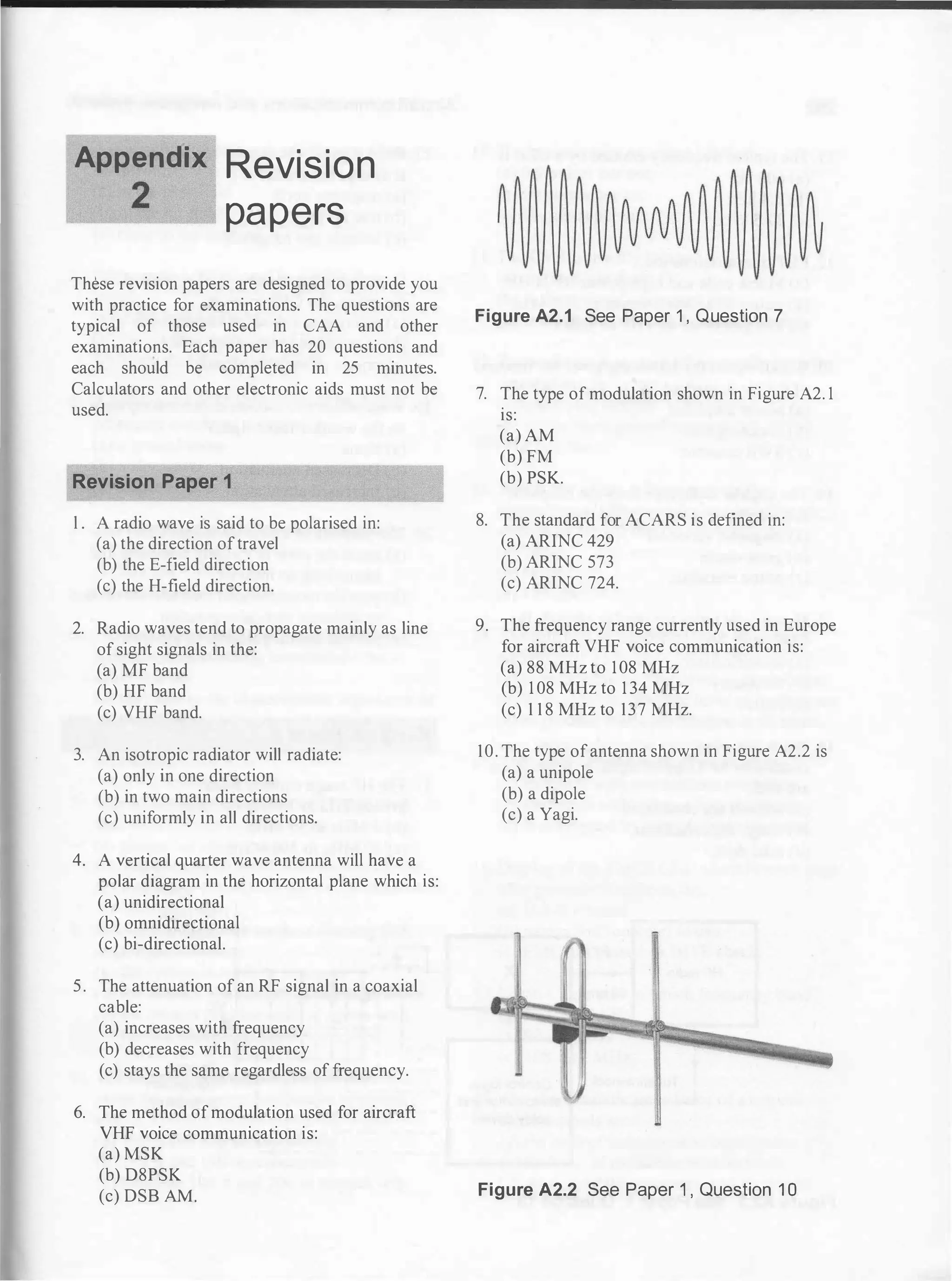
.......-.Ah Piol
3eve!IOO Angle 0.0 deg. Goin
Olier Rng 2.16 dBI
Slce Max Goin 2.16 dEll @ Az Angle = 0.0 deg.
�-. 99.99 d8
Beomwidth 77 4 deg.; -3d8 @ 321 .3, 38.7 deg.
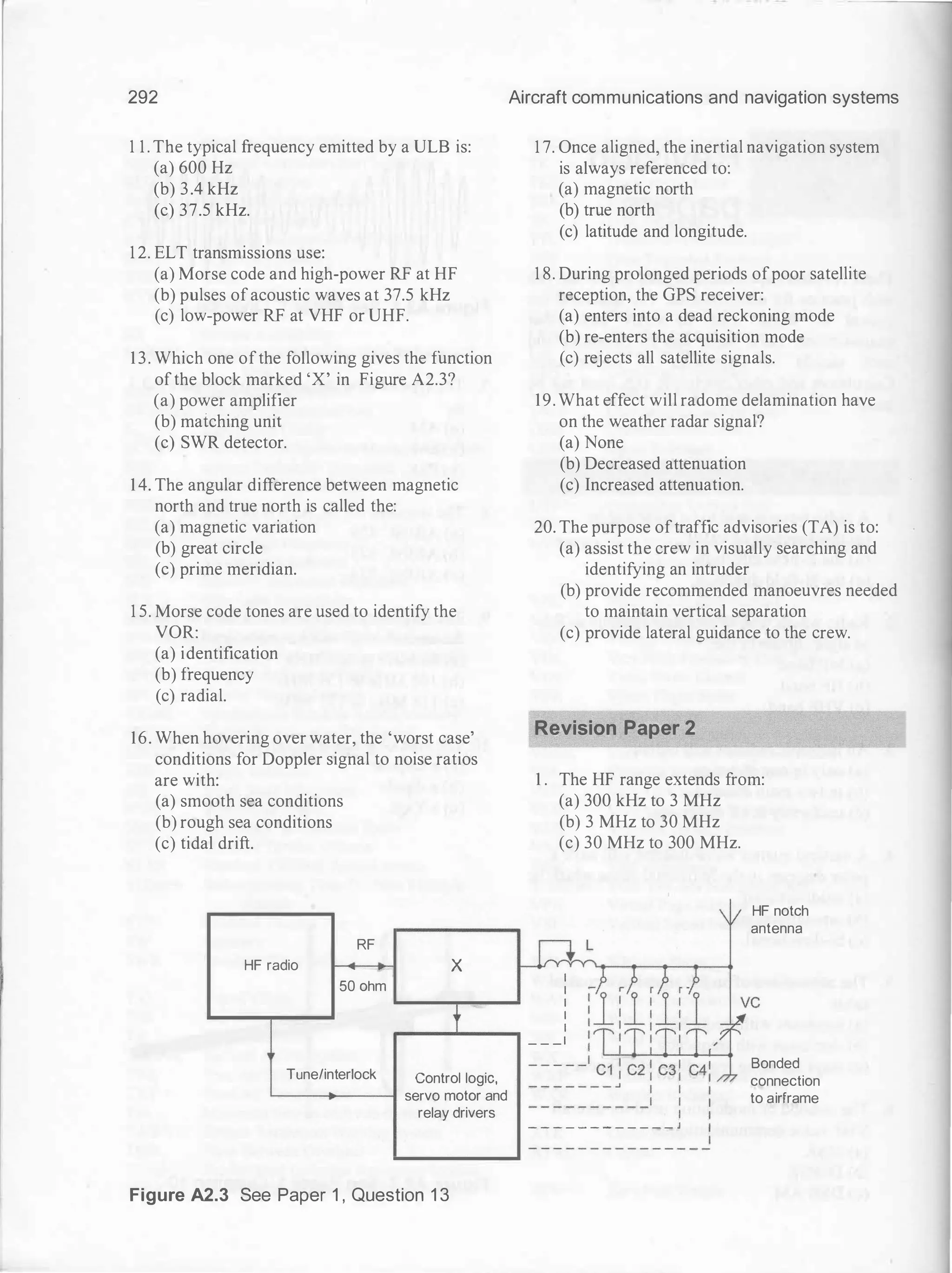
Stdelobo Goln 2.16 dBI @ Az Angle = 1 80.0 deg.
�tOrtJSidelobe o.o dB
EZNEC Demo
299.793 111Hz
0.0 deg.
2.16 cfli
0.0 dBmax
Figure 2.5 E-field polar radiation pattern for
a half-wave dipole
,. 20 Plot. Cardioid r;;]LQJL8J
=.e Edit View
Total Aeld
o.=mih Piol
3e'<SXln Angle 0.0 deg.
Juer Ring 1 64 dBi
Slce Max Goin 1 .64 dEll @ Az Angle = 185.0 deg.
�.m.eocl< 0.02 d8
Seomwldlh ?
ScelobeGoln 1 .64 dBi @ Az Angle = 354.0 deg.
='O!'tJSidelobo 0.0 dB
EZNEC Demo
299.793 111Hz
315.0deg.
1 42 dBi
-022 d8max
Figure 2.6 H-field polar radiation pattern for
a half-wave dipole
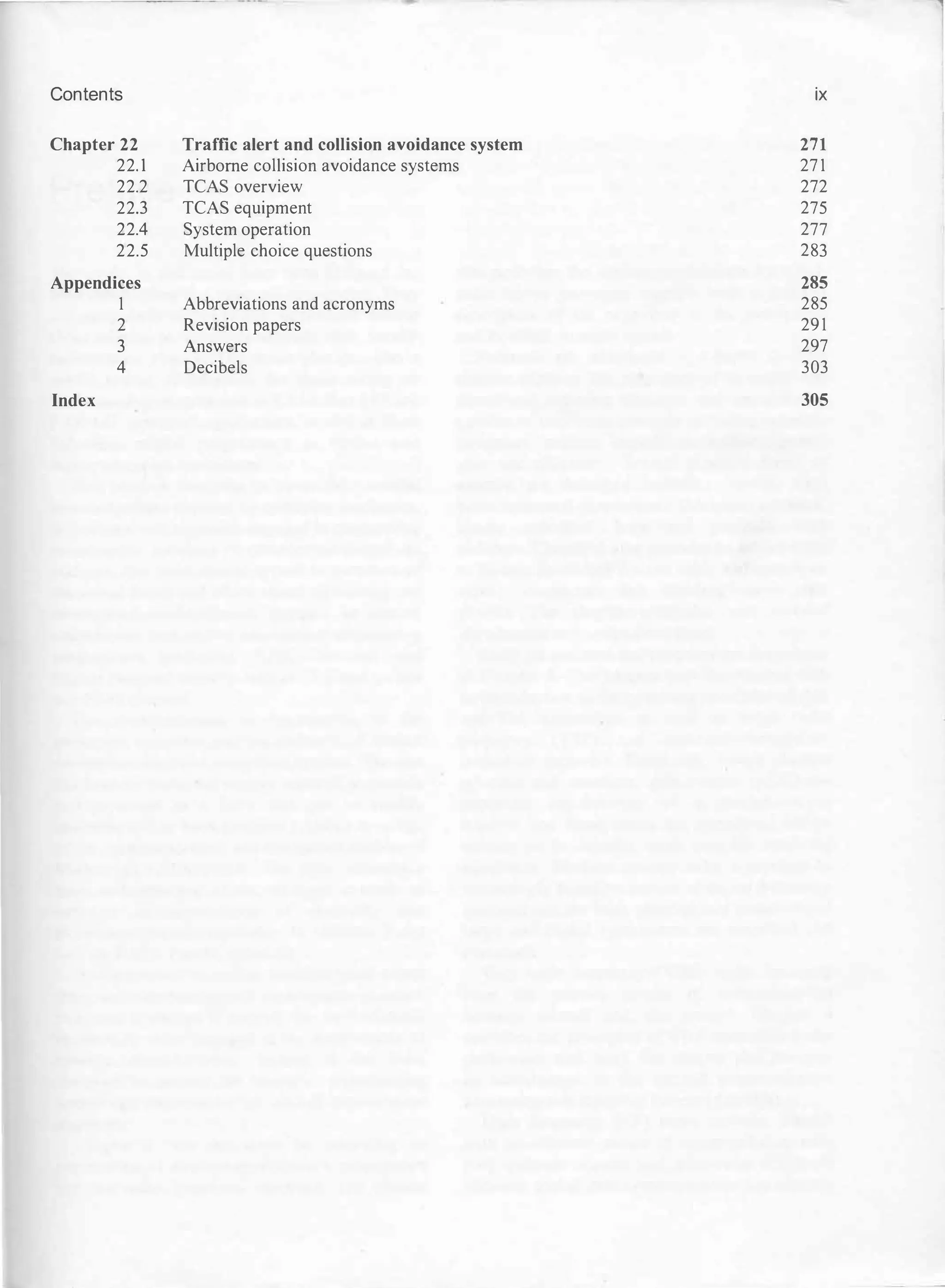
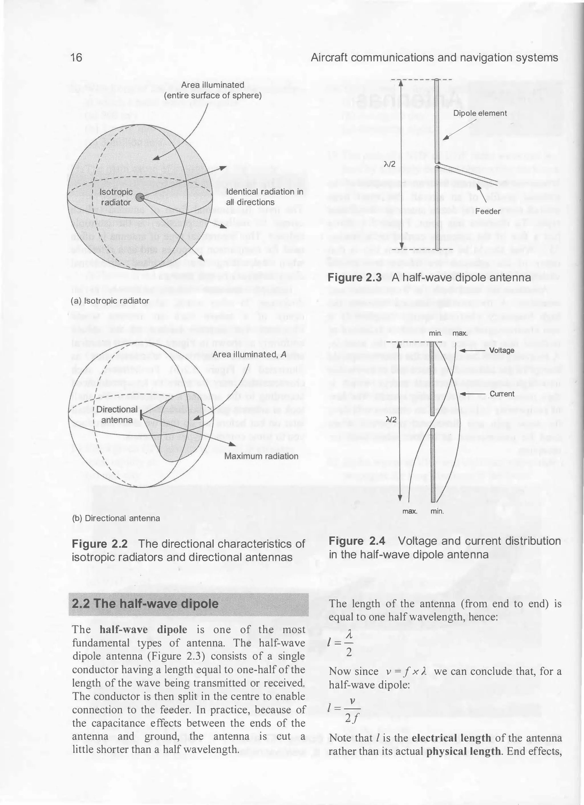
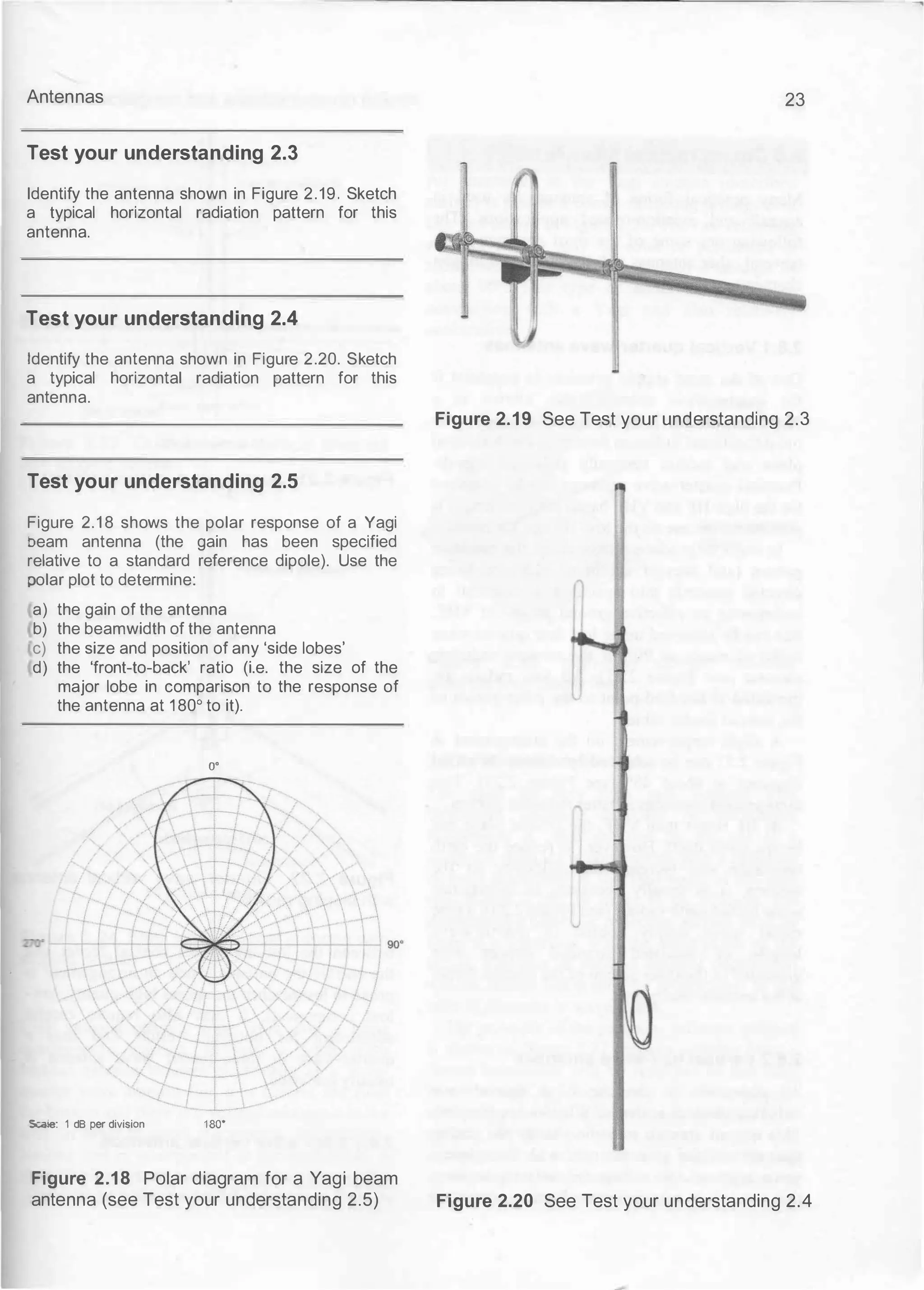
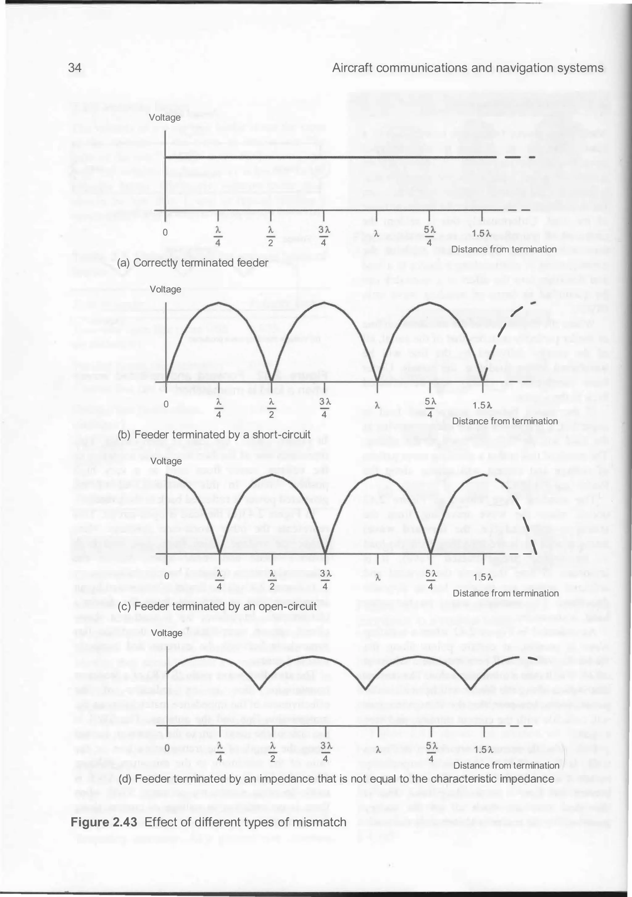
or capacitance effects at the ends of the antenna
::equire that we reduce the actual length of the
erial and a 5% reduction in length is typically
:equired for an aerial to be resonant at the centre
of its designed tuning range.
Figure 2.4 shows the distribution of current
and voltage along the length of a half-wave
dipole aerial. The current is maximum at the
;::entre and zero at the ends. The voltage is zero at
:he centre and maximum at the ends. This
1 7
Iii 3D Plot: Dipole in free space c;J(g]�
File Edit View Options Reset
rHighlight-- .--
-
-
-
-
-
-
-
-
-=
E
=
z
N
""
E
""'
C
.,.
Oe
_
m
_
o
--1
(' Off
(' 8zimuth Slice
(o' E]ev Slice Y
,,·0 360
_ill_-..cl
0
SliceAzimuth
1 180
0
J ·180
II Cursor Elev
l___ - -
P' _2how 2D Plot
Figure 2.7 30 polar radiation pattern for a
half-wave dipole (note the 'doughnut' shape)
implies that the impedance is not constant along
the length ofaerial but varies from a maximum at
the ends (maximum voltage, minimum current)
to a minimum at the centre.
The dipole antenna has directional properties
illustrated in Figures 2.5 to 2.7. Figure 2.5 shows
the radiation pattern of the antenna in the plane
of the antenna's electric field (i.e. the E-field
plane) whilst Figure 2.6 shows the radiation
pattern in the plane of the antenna's magnetic
field (i.e. the H-field plane).
The 3D plot shown in Figure 2.7 combines
these two plots into a single 'doughnut' shape.
Things to note from these three diagrams are
that:
• in the case of Figure 2.5 minimum radiation
occurs along the axis ofthe antenna whi1st the
two zones of maximum radiation are at 90°
(i.e. are 'normal to') the dipole elements
• in the case of Figure 2.6 the antenna radiates
uniformly in all directions.
Hence, a vertical dipole will have omni
directional characteristics whilst a horizontal
dipole will have a bi-directional radiation
pattern. This is an important point as we shall see
later.](https://image.slidesharecdn.com/aircraftcommunicationsandnavigationsystemsprinciplesoperationandmaintenancepdfdrive-250205173033-c029e156/75/Aircraft-communications-and-navigation-systems_-principles-operation-and-maintenance-PDFDrive-pdf-27-2048.jpg)
![22
{b) Light analogy
{c) Directional pattern
·�·
Figure 2.15 Light analogy for the four
element Vagi shown in Figure 2.1 4
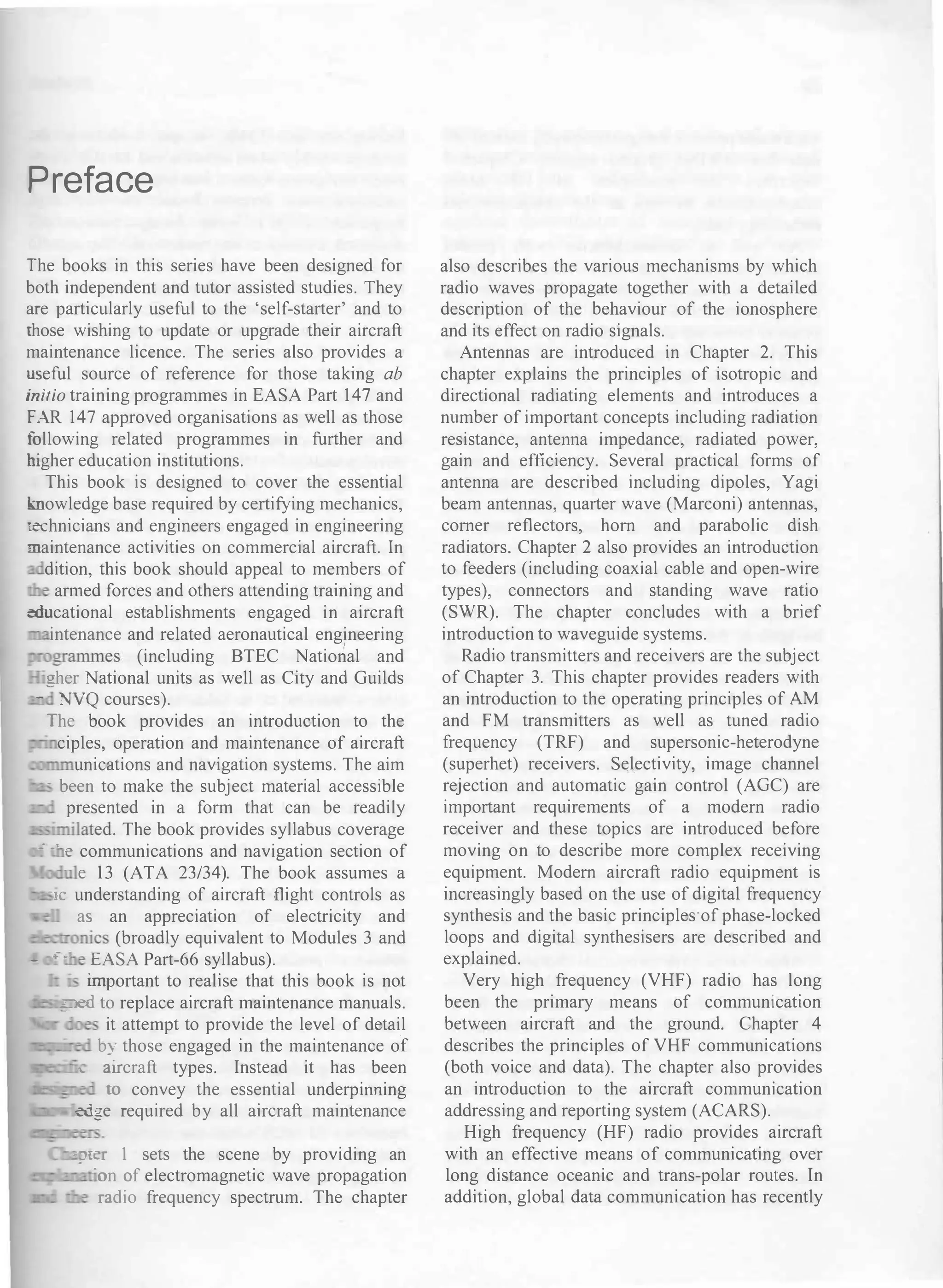
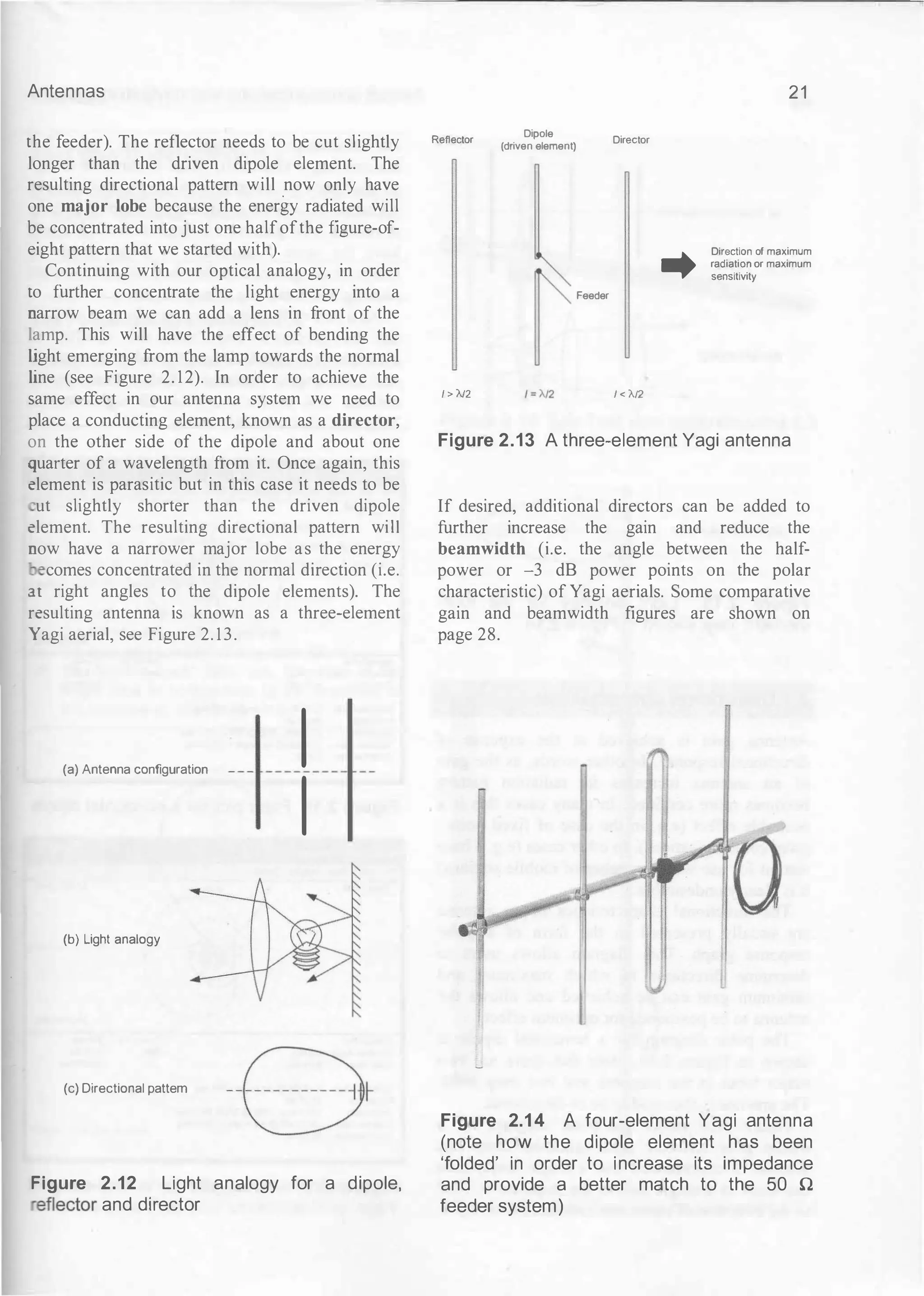
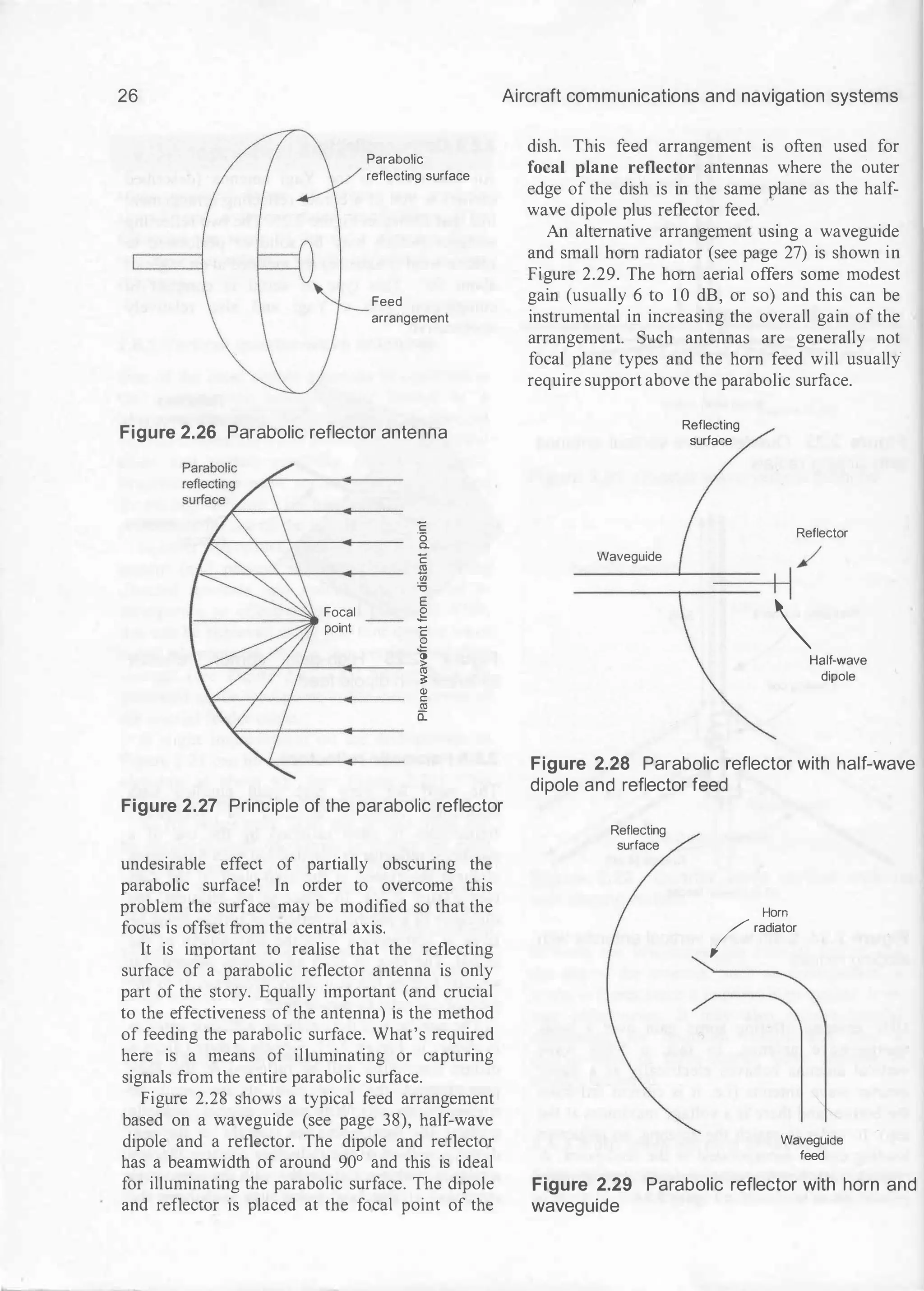
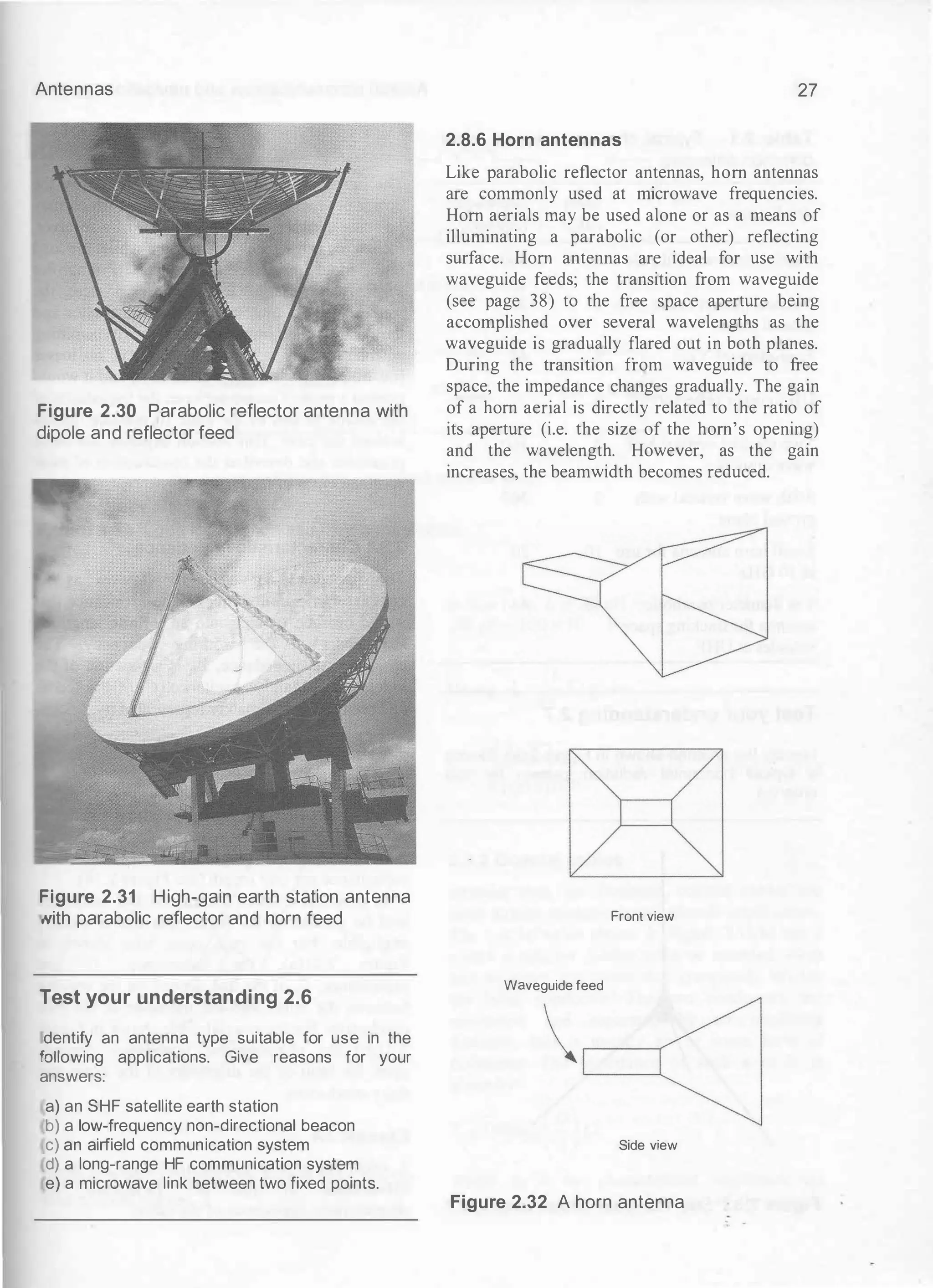
2 .7 Directional characteristics
Antenna gain is achieved at the expense of
directional response. In other words, as the gain
of an antenna increases its radiation pattern
becomes more confined. In many cases this is a
desirable effect (e.g. in the case of fixed point
point communications). In other cases (e.g. a base
station for use with a number of mobile stations)
it is clearly undesirable.
The directional characteristics of an antenna
are usually presented in the form of a polar
response graph. This diagram allows users to
determine directions in which maximum and
minimum gain can be achieved and allows the
antenna to be positioned for optimum effect.
The polar diagram for a horizontal dipole is
shown in Figure 2. 1 6. Note that there are two
major lobes in the response and two deep nulls.
The antenna is thus said to be bi-directional.
Figure 2. 1 7 shows the polar diagram for a
dipole plus reflector. The radiation from this
antenna is concentrated into a single major lobe
and there is a single null in the response at 1 80°
to the direction of maximum radiation.
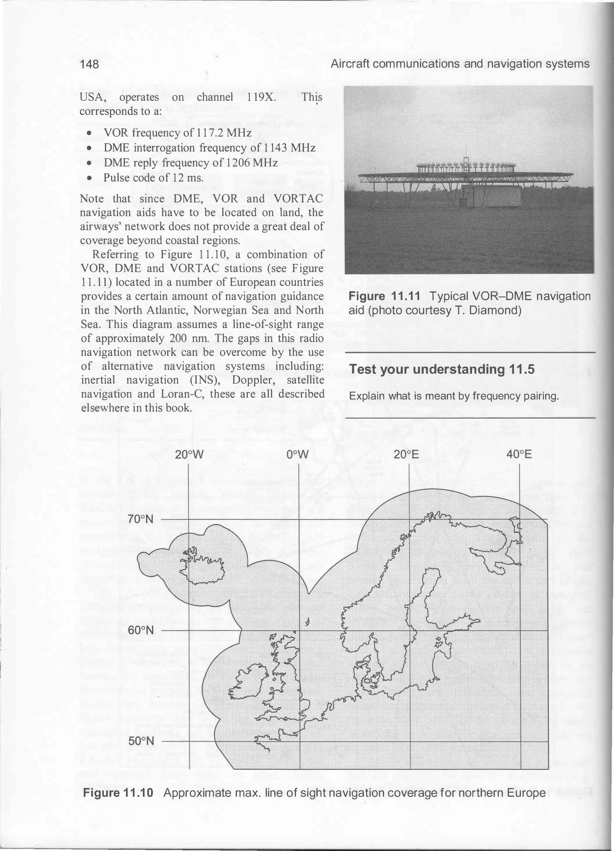
Aircraft communications and navigation systems
An alternative to improving the gain but
maintaining a reasonably wide beamwidth is that
of stacking two antennas one above another (see
Figure 2.20). Such an arrangement will usually
provide a 3 dB gain over a single antenna but will
have the same beamwidth. A disadvantage of
stacked arrangements is that they require accurate
phasing and matching arrangements.
As a rule of thumb, an increase in gain of 3 dB
can be produced each time the number of
elements is doubled. Thus a two-element antenna
will offer a gain of about 3 dBd, a four-element
antenna will produce 6 dBd, an eight-element
Yagi will realise 9 dBd, and so on.
"' 20 Plot: Dipole in free space
GJLQ]�
File Edit View
• Total Field
Azimuth Plot
Elevation Angle 0.0 deg.
Outer Ring 2.16 dBI
Slice Max Gain 2.16 dBi @ Az Angle = 0.0 deg.
Front/Side 99.99 d8
Beomwidth 77.4 deg; -3dB @ 321.3, 38.7 deg.
Sidelobe Gain 2.1 6 d8i @ Az Angle = 180D deg.
Fronii.Sidolobe 0.0 dB
Gain
EZNEC Demo
299.793 MHz
0.0 deg.
2.16 oBi
0.0 dBme.x
Figure 2.1 6 Polar plot for a horizontal dipole
"' 20 Plot. Cardioid
GJ(QJ�
File Edi
t View
� Total Field
Azim..th Piot
Elevotioo Angie 0.0 deg.
OuterRilg 8.19 dBi
Slice Mox ooin 8.1 9 d8i @ Az Angle = O.O deg.
Frori.eock 3521 d8
Beamwfdth 1 78.4 deg.; -3dB @ 270.8, 89.2 deg.
Sidelobe Gain -27.02 dBi @ Az Angle = 1 60.0 deg.
FrontiSidelobe 35.21 dB
EZNEC Demo
299.793 h4Hz
0.0 deg.
8.19 d8i
0.0 d8mox
Figure 2.17 Polar plot for a two-element
Vagi](https://image.slidesharecdn.com/aircraftcommunicationsandnavigationsystemsprinciplesoperationandmaintenancepdfdrive-250205173033-c029e156/75/Aircraft-communications-and-navigation-systems_-principles-operation-and-maintenance-PDFDrive-pdf-32-2048.jpg)
![Antennas
Resistance, R Reactance, X
50 .---��--�----.-------.-�----.---�--.-------e 50
SWR SWR
3 40 !----�+-----t--;----;c:::-"'""""'-,--'---'---+-+--,--'-----l-+-+--'--------l 40 3
2.5 30
2 20
]_
0
1 17.5 120 122.5 125
Frequency (MHz)
127.5 1 30
0
1 32.5
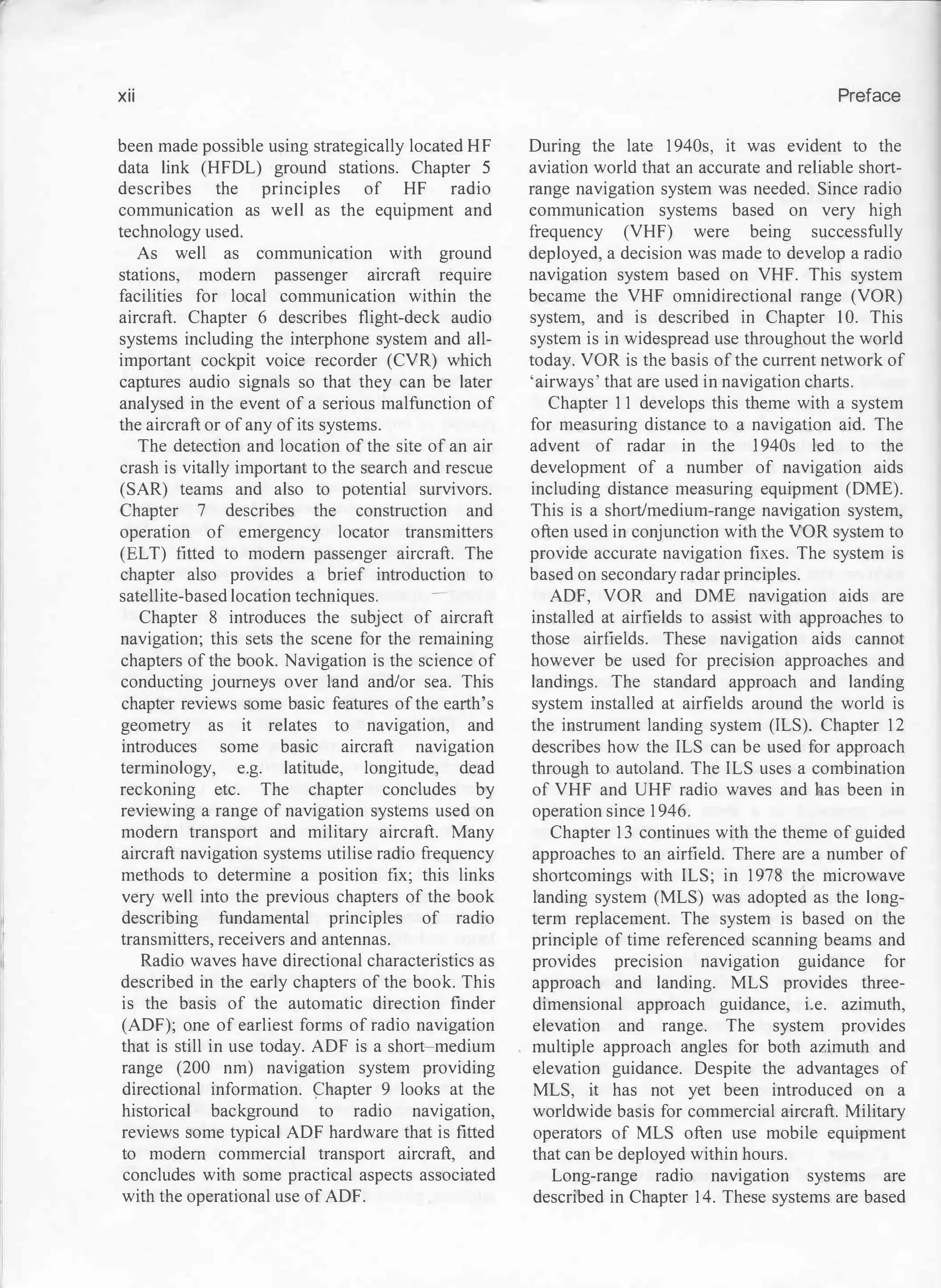
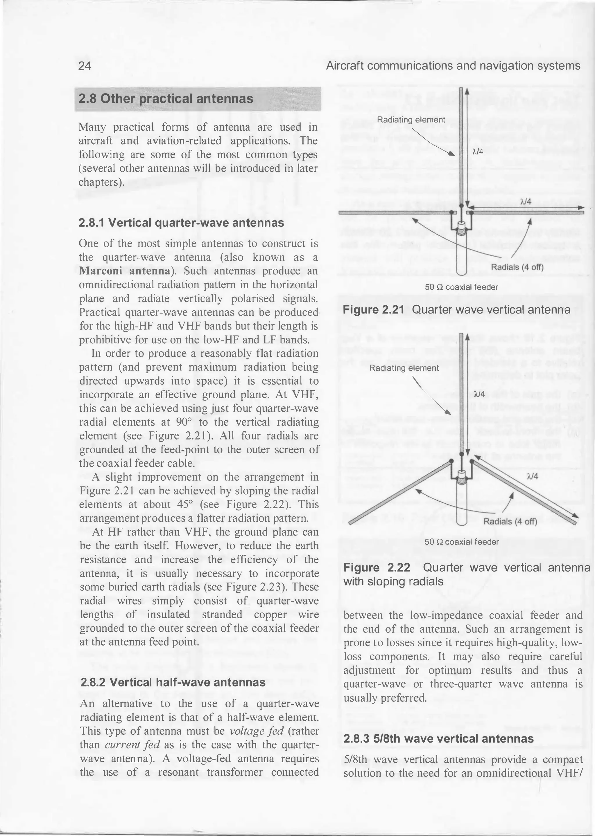
Figure 2.52 See Test your knowledge 2.9
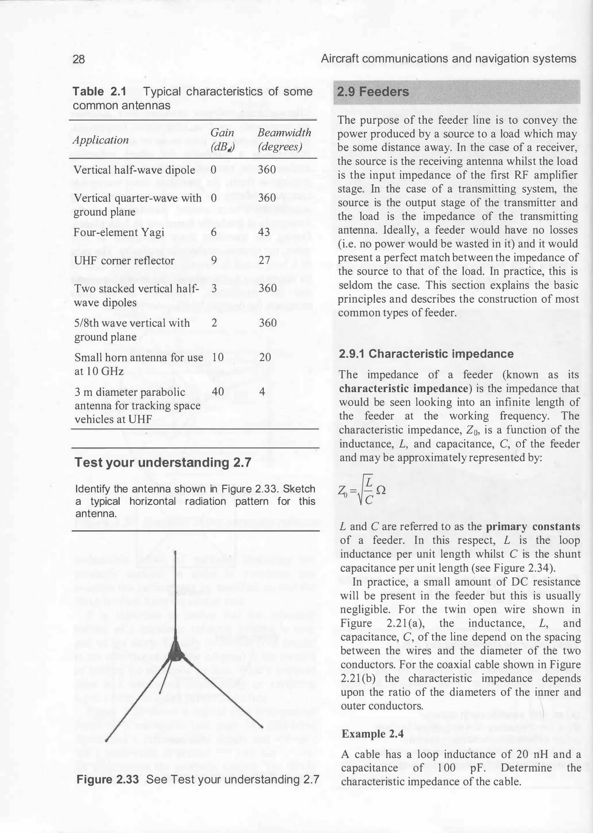
Test your understanding 2.9
l=igure 2.52 shows the frequency response of a
ertical quarter-wave antenna used for local VHF
communications. Use the graph to determine the
<allowing:
a) The frequency at which the SWR is minimum
'b) The 2:1 SWR bandwidth of the antenna
c) The reactance of the antenna at 1 20 MHz
d) The resistance of the antenna at 1 20 MHz
e) The frequency at which the reactance of the
antenna is a minimum
2.13 Multiple choice questions
1 . An isotropic radiator will radiate:
(a) only in one direction
(b) in two main directions
(c) uniformly in all directions.
2. Another name for a quarter-wave vertical
antenna is:
(a) a Yagi antenna
(b) a dipole antenna
(c) a Marconi antenna.
39
f) The frequency at which the resistance of the
antenna is 50 n.
3. A full-wave dipole fed at the centre must be:
(a) current fed
Test your understanding 2.10
Explain what is meant by standing wave ratio
SWR) and why this is important in determining
"he performance of an antenna/feeder
combination.
(b) voltage fed
(c) impedance fed.
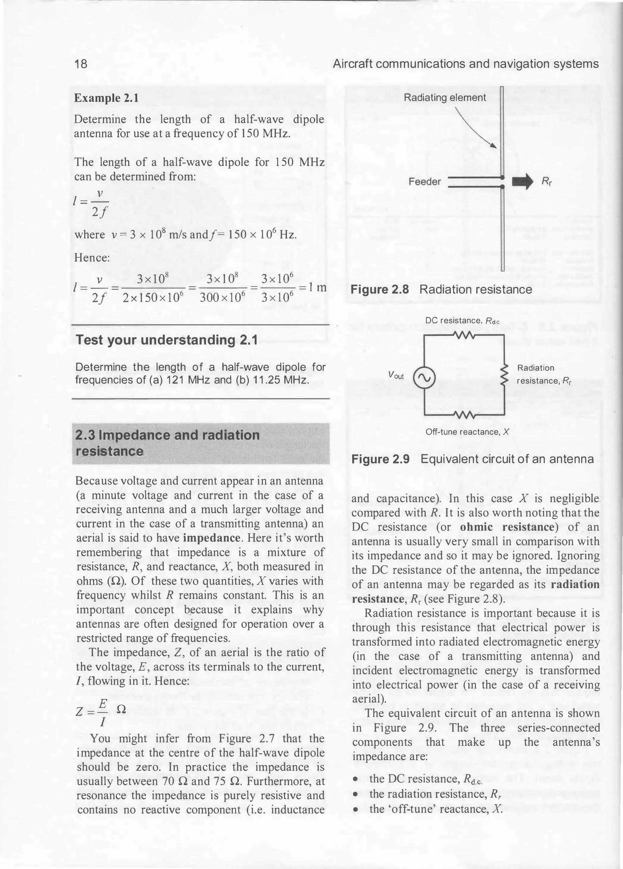
4. The radiation efficiency ofan antenna:
(a) increases with antenna loss resistance
(b) decreases with antenna loss resistance
(c) is unaffected by antenna loss resistance.](https://image.slidesharecdn.com/aircraftcommunicationsandnavigationsystemsprinciplesoperationandmaintenancepdfdrive-250205173033-c029e156/75/Aircraft-communications-and-navigation-systems_-principles-operation-and-maintenance-PDFDrive-pdf-49-2048.jpg)
!['
"i
42 Aircraft communications and navigation systems
The BFO can be above or below the incoming _j�M��n� ��� nfln���M_jnn_
signal frequency by an amount that is equal to the -�ijijijijijijijijijv�ijijijijijijijijijv
beat frequency (i.e. the audible signal that results
from the 'beating' of the two frequencies and - • - e
which appears at the output of the detector stage).
Hence, ]sFO =!RF±]AF
from which:
}sFO = (162.5 ± 1 .25) kHz = 1 60.75 or 1 63.25 kHz
Test your understanding 3.1
An audio frequency signal of 850 Hz is produced
when a BFO is set to 455.5 kHz. What is the input
signal frequency to the detector?
3.1 .1 Morse code
Transmitters and receivers for CW operation are
extremely simple but nevertheless they can be
extremely efficient. This makes them particularly
useful for disaster and emergency communication
or for any situation that requires optimum use of
low power equipment. Signals are transmitted
using the code invented by Samuel Morse (see
Figures 3 .2 and 3.3).
A · - N - ·
B - · · · 0 - - -
c - · - · p · - - ·
D - · · Q - - · -
E • R · - ·
F · · - · s • • •
G - - · T -
H • • • • u · · -
I • • v · · · -
J · - - - w · - -
K - · - X - · · -
L · - · · y - · - -
M - - z - - · ·
1 · - - - - 6 - · · · ·
2 · · - - - 7 - - · · ·
3 · · · - - 8 - - - · ·
4 · · · · - 9 - - - - ·
5 • • • • • 0 - - - - -
Figure 3.2 Morse code
c
Figure 3.3 Morse code signal for the letter C
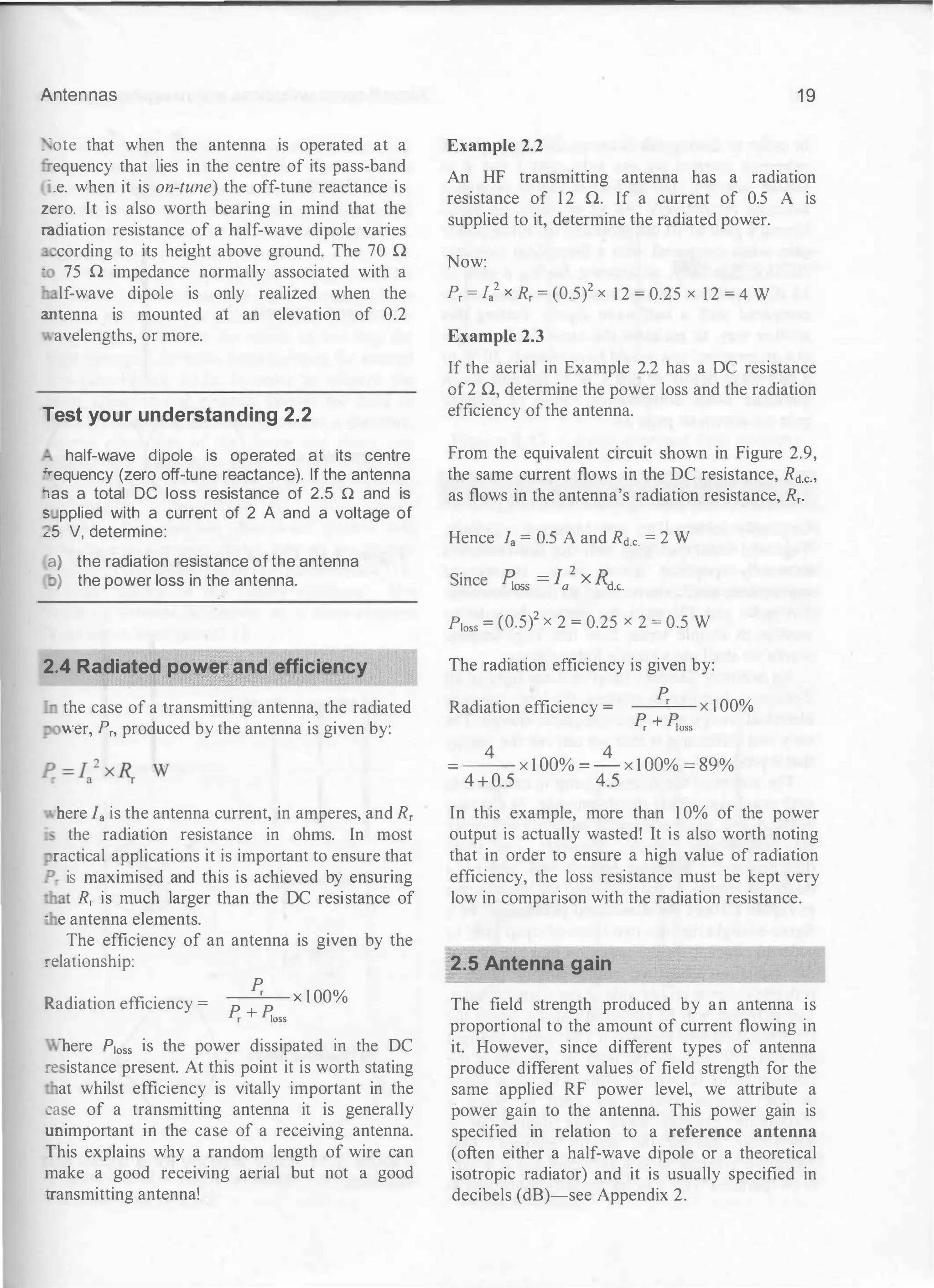
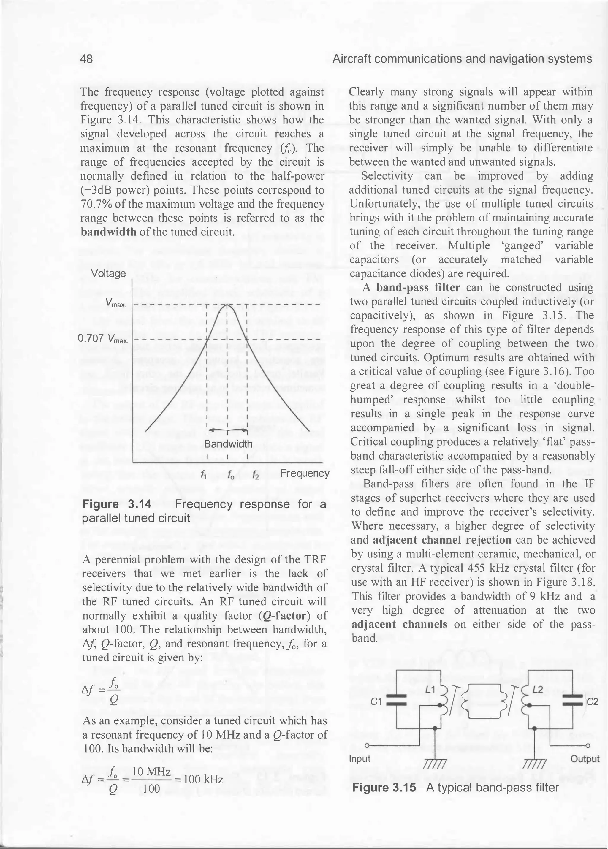
3.2 Modulation and demodulation
In order to convey information using a radio
frequency carrier, the signal information must be
superimposed or 'modulated' onto the carrier.
Modulation is the name given to the process of
changing a particular property of the carrier wave
in sympathy with the instantaneous voltage (or
current) signal.
The most commonly used methods of
modulation are amplitude modulation (AM) and
frequency modulation (FM). In the former case,
the carrier amplitude (its peak voltage) varies
according to the voltage, at any instant, of the
modulating signal. In the latter case, the carrier
frequency is varied in accordance with the
voltage, at any instant, ofthe modulating signal.
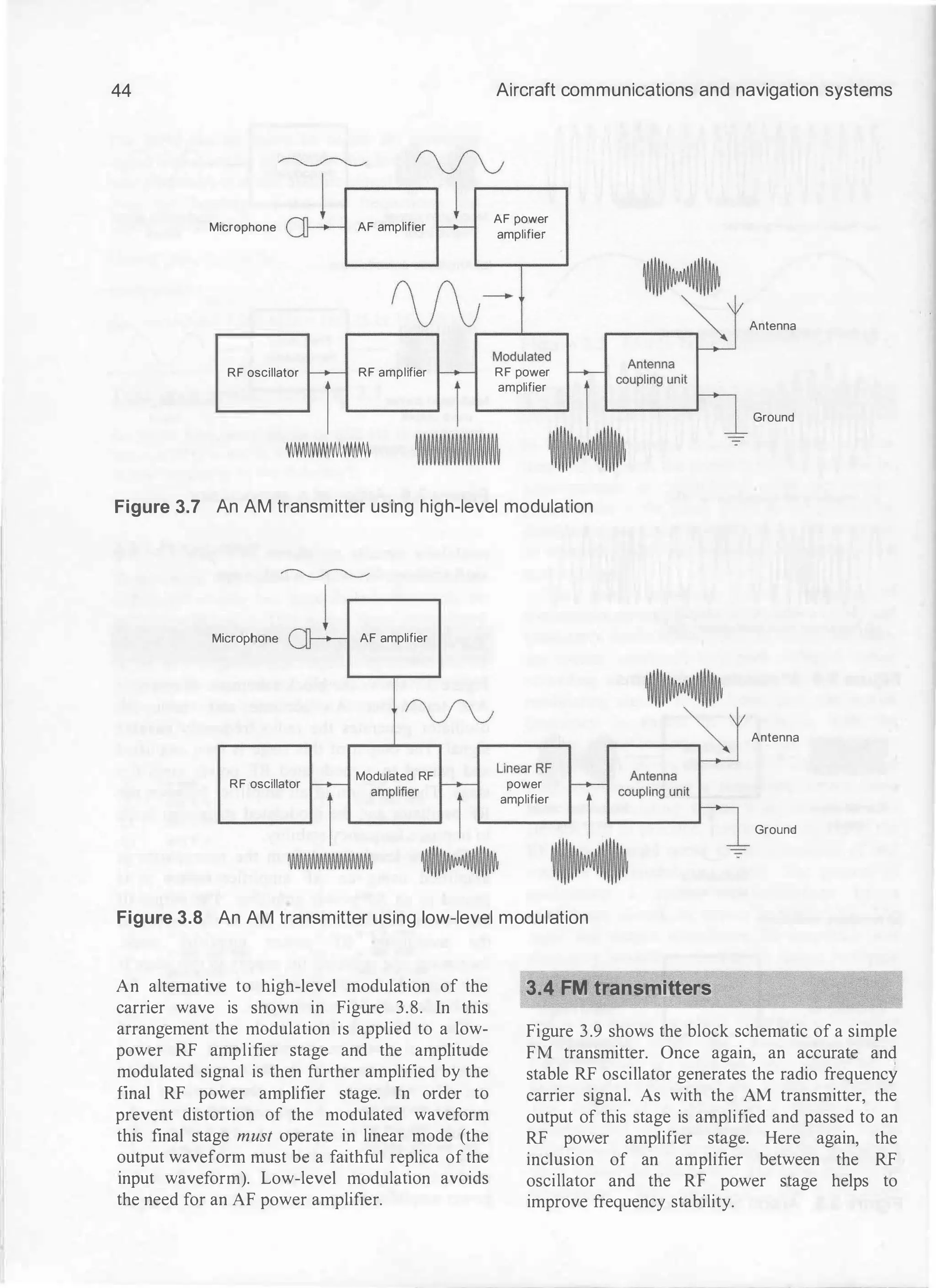
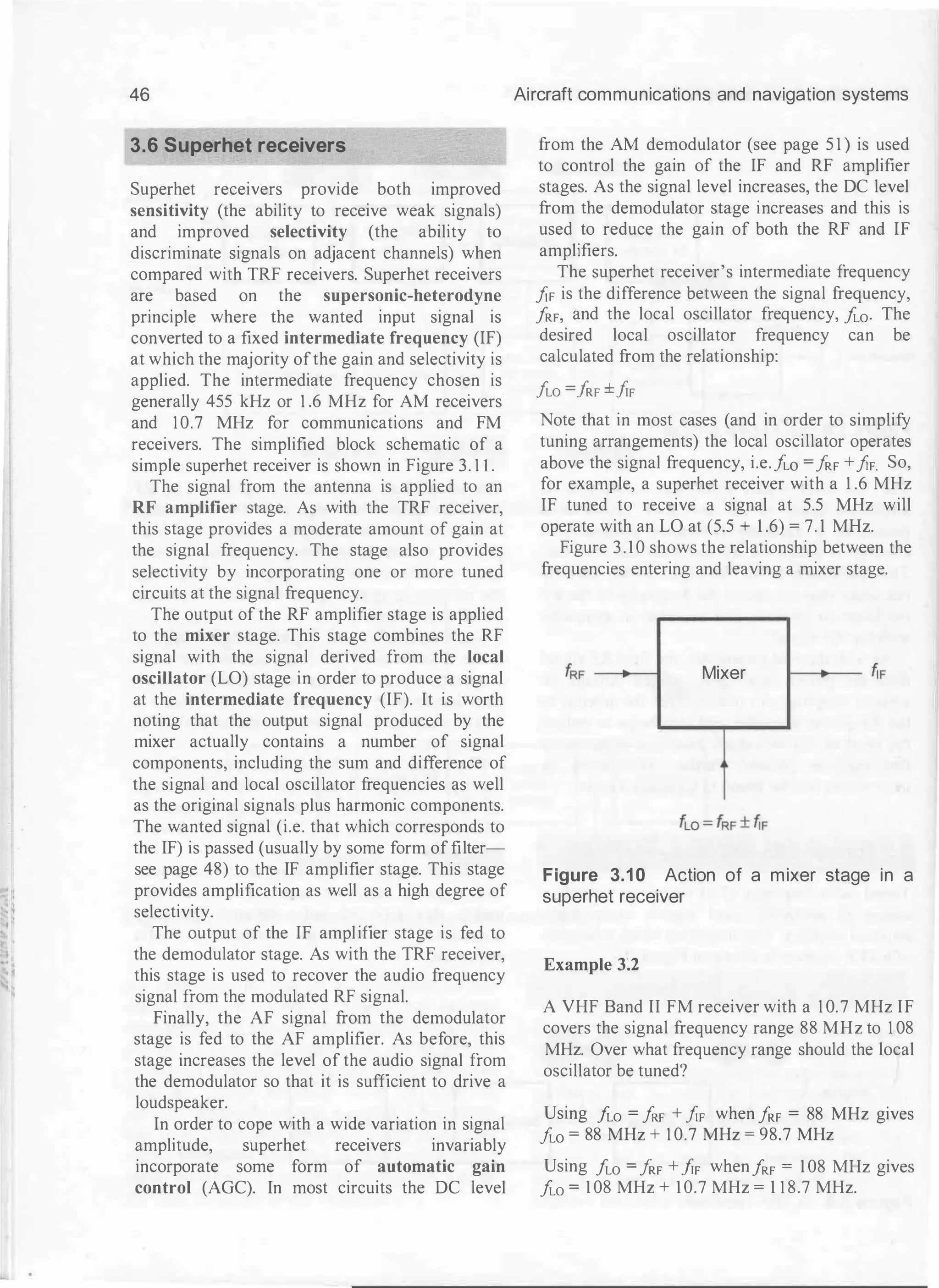
Figure 3.4 shows the effect of amplih1de and
frequency modulating a sinusoidal carrier (note
that the modulating signal is in this case also
sinusoidal). In practice; many more cycles of the
RF carrier would occur in the time-span of one
cycle of the modulating signal. The process of
modulating a carrier is undertaken by a
modulator circuit, as shown in Figure 3.5. The
input and output waveforms for amplitude and
frequency modulator circuits are shown in Figure
3.6.
Demodulation is the reverse of modulation
and is the means by which the signal information
is recovered from the modulated carrier.
Demodulation is achieved by means of a
demodulator (sometimes also called a detector).
The output of a demodulator consists of a
reconstructed version of the original signal
information present at the input of the modulator
stage within the transmitter. The input and output
waveforms for amplitude and frequency](https://image.slidesharecdn.com/aircraftcommunicationsandnavigationsystemsprinciplesoperationandmaintenancepdfdrive-250205173033-c029e156/75/Aircraft-communications-and-navigation-systems_-principles-operation-and-maintenance-PDFDrive-pdf-52-2048.jpg)
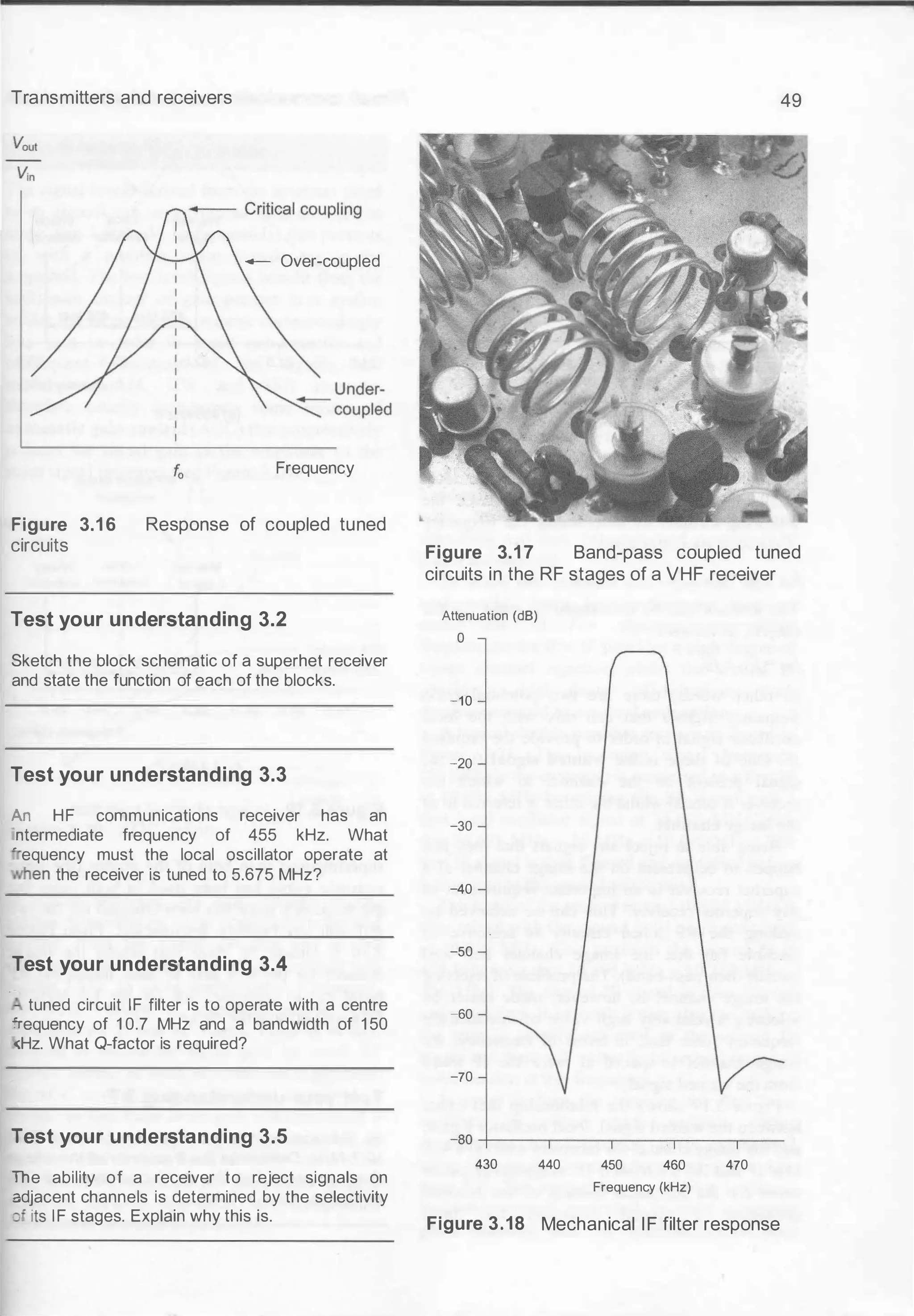


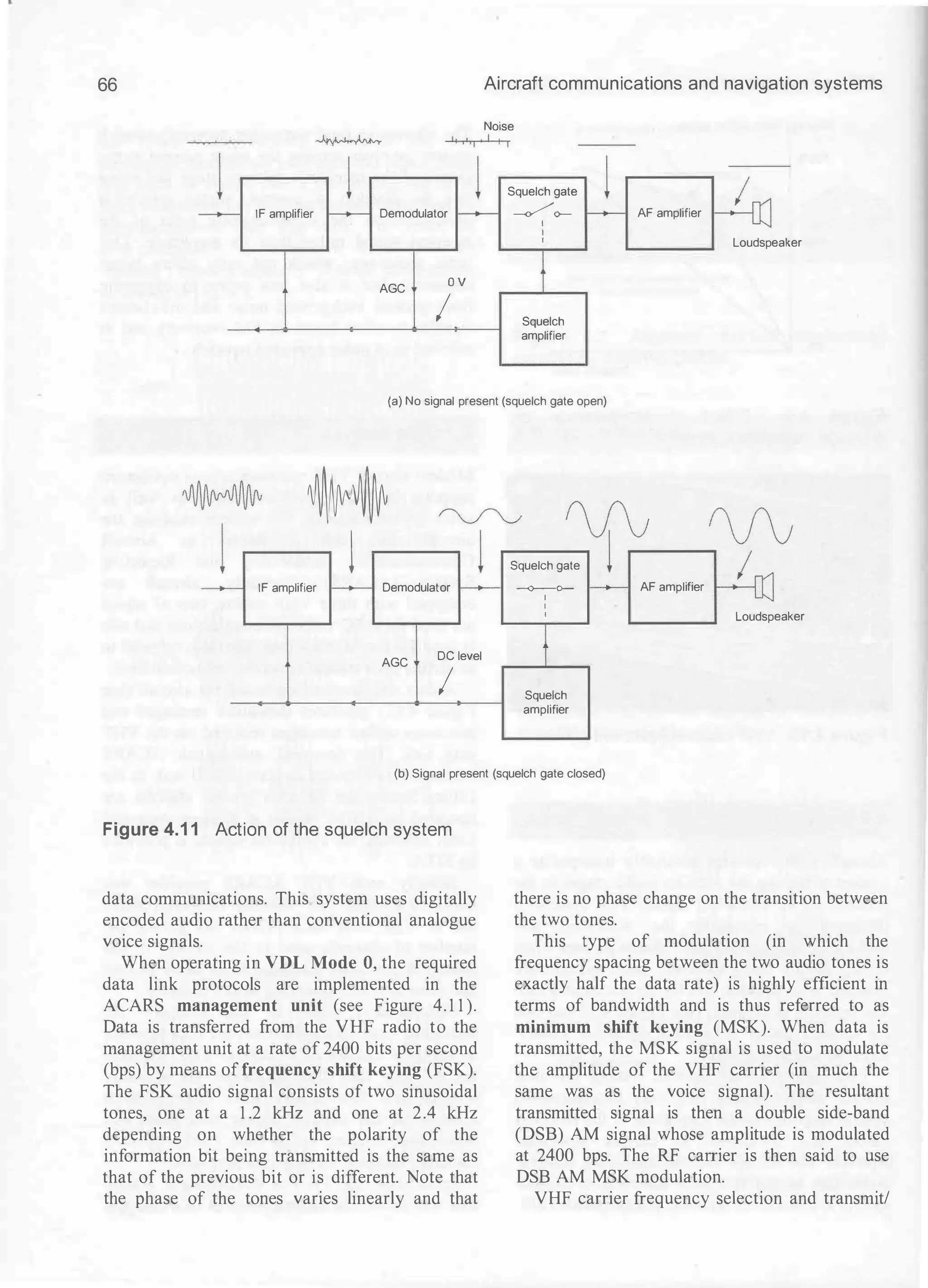
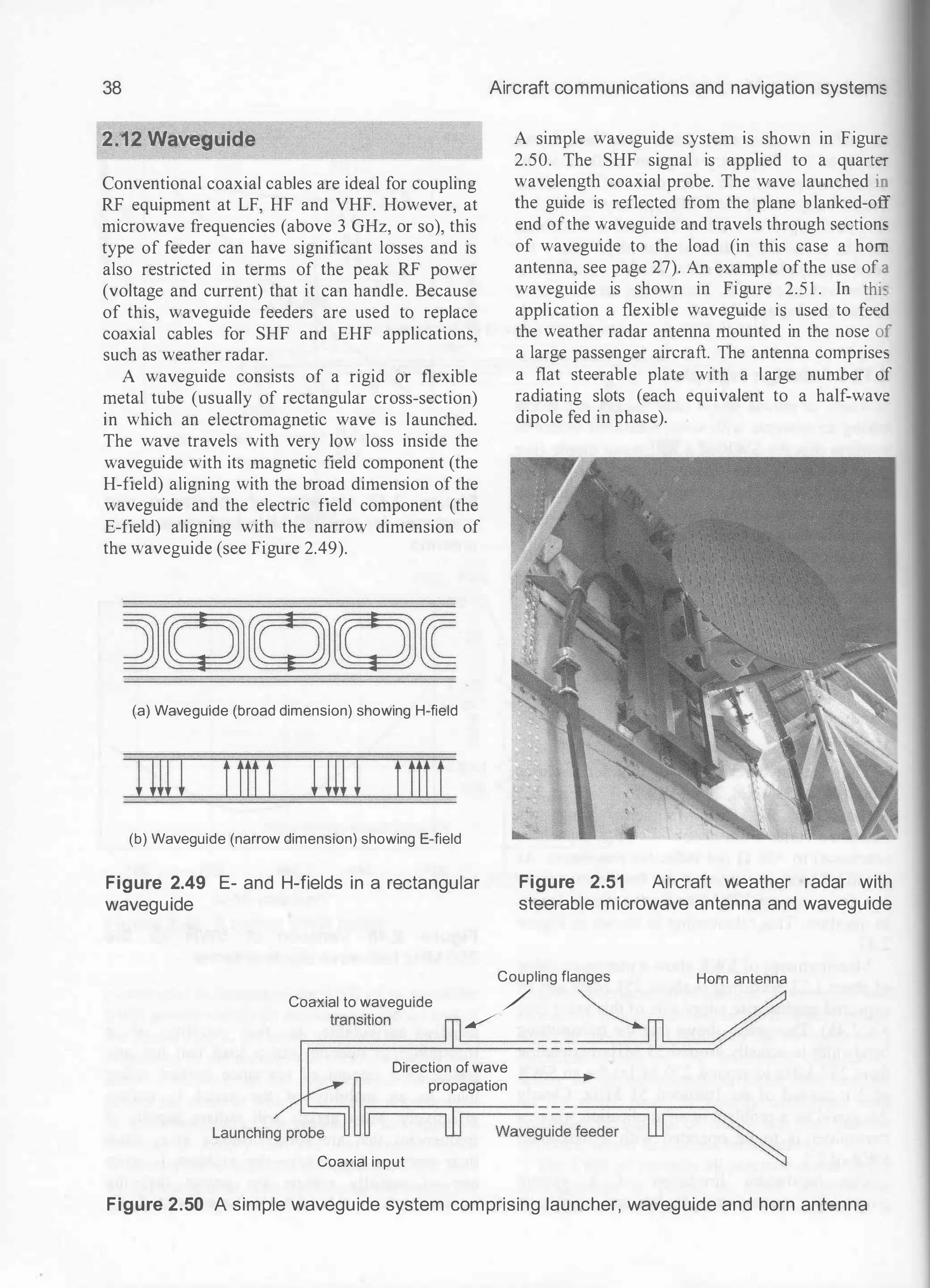
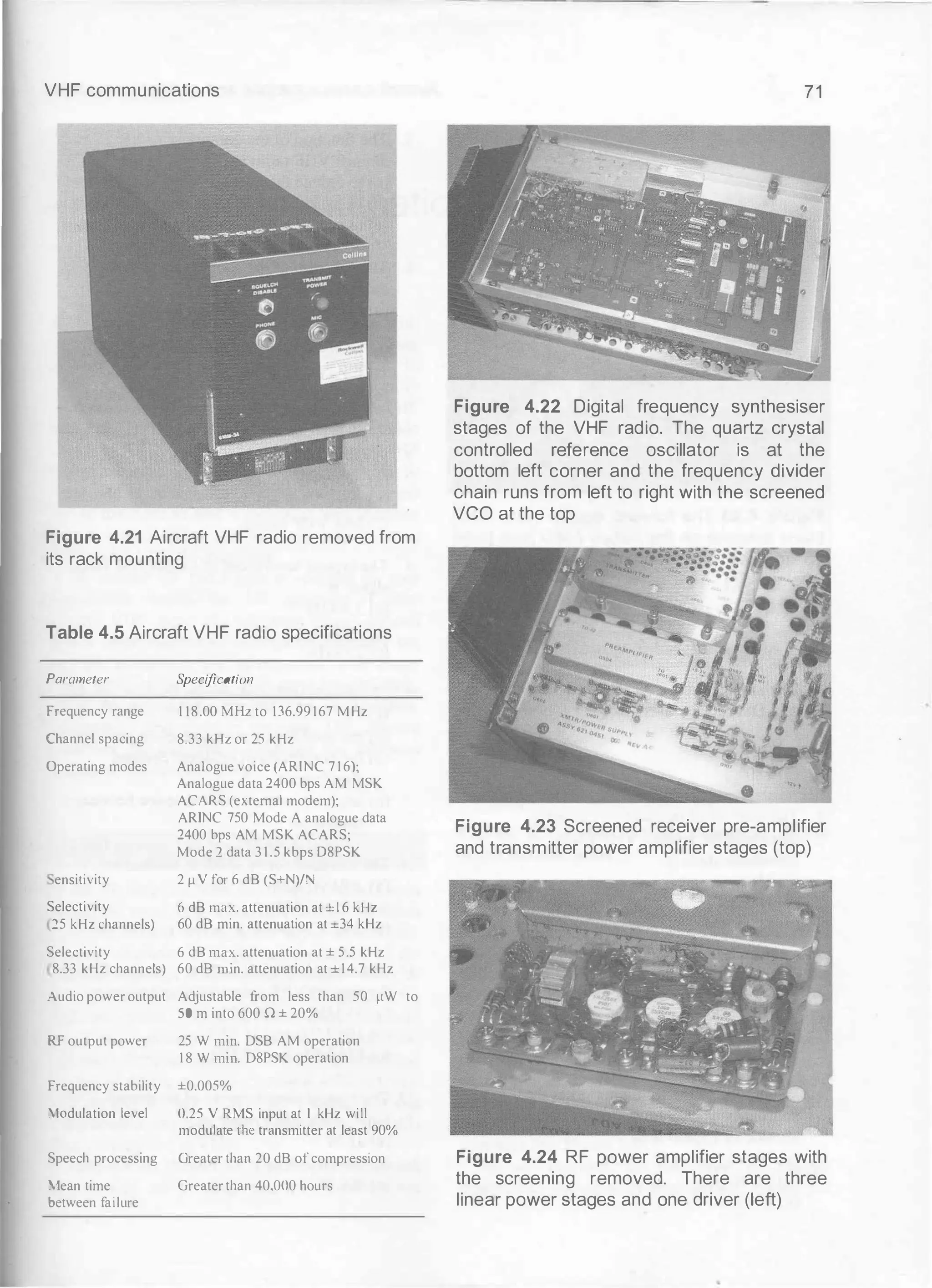
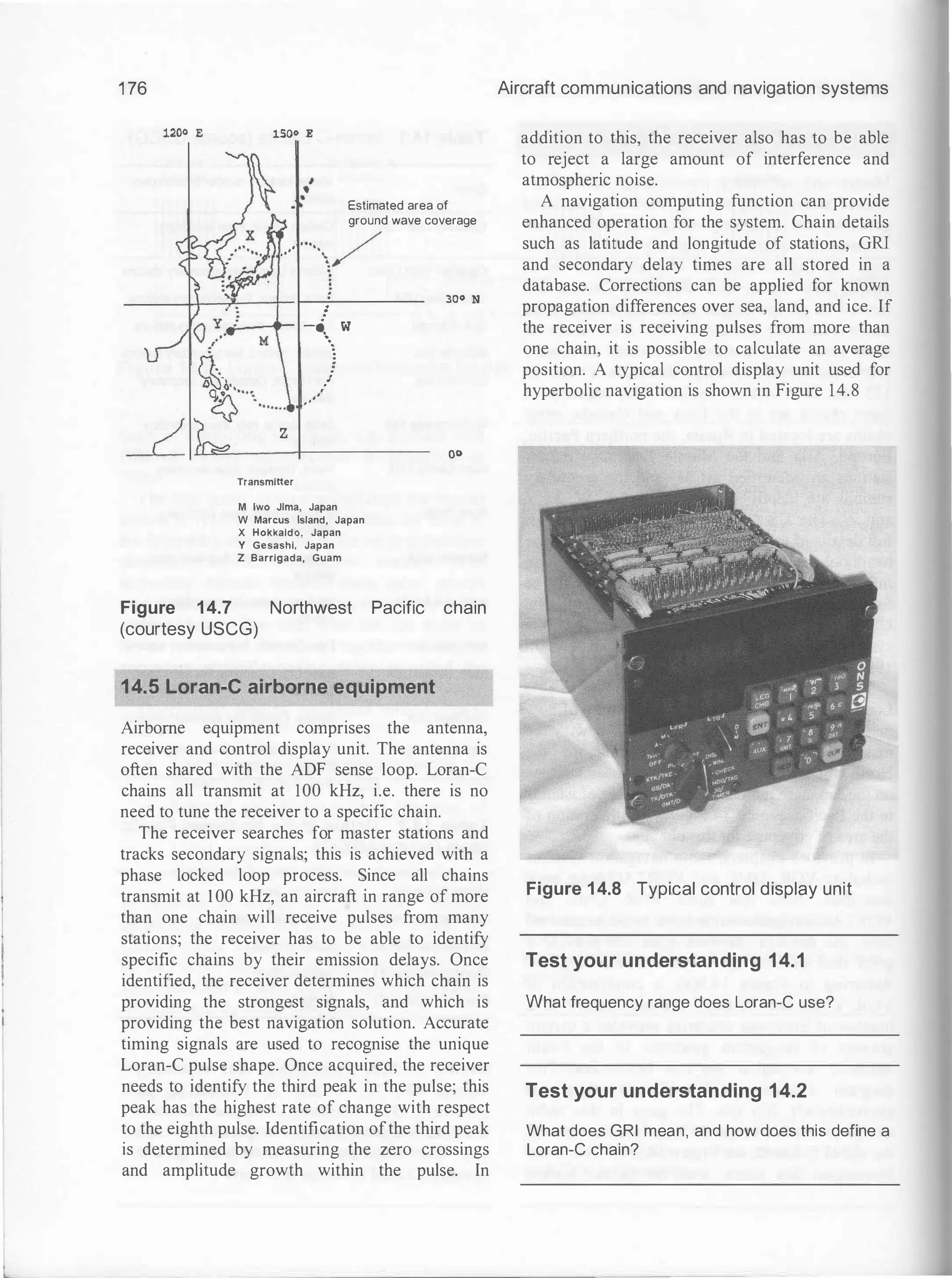
![VHF communications
in the aircraft. The aircraft ACARS components
include a management unit (see Figure 4. 12)
which deals with the reception and transmission
of messages via the VHF radio transceiver, and
the control unit which provides the crew
interface and consists of a display screen and
printer. The ACARS ground network comprises
the ARlNC ACARS remote transmitting/
receiving stations and a network of computers
and switching systems. The ACARS command,
control and management subsystem consists of
the ground-based airline operations and
associated functions including operations control,
maintenance and crew scheduling.
There are two types of ACARS messages;
downlink messages that originate from the
aircraft and uplink messages that originate from
ground stations (see Figures 4. 14 to 4. 17).
Frequencies used for the transmission and
reception of ACARS messages are in the band
extending from 129 MHz to 137 MHz (VHF) as
shown in Table 4.4. Note that different channels
are used in different parts of the world. A typical
ACARS message (see Figure 4. 14) consists of:
• mode identifier (e.g. 2)
• aircraft identifier (e.g. G-DBCC)
• message label (e.g. SU-a weather request)
• block identifier (e.g. 4)
• message number (e.g. M55A)
• flight number (e.g. BD0 1NZ)
• message content (see Figure 4. 1 4).
Table 4.4 AGARS channels
Frequency ACARS service
129. 1 25 MHz USA and Canada (additional)
130.025 MHz USA and Canada (secondary)
150.450 MHz USA and Canada (additional)
1 3 l . l25 MHz USA (additional)
1 3 1 .475 MHz Japan (primary)
1 3 1 .525 MHz Europe (secondary)
1 3 1 .550 MHz USA, Canada, Australia (primary)
1 3 1 .725 MHz Europe (primary)
1 36.900 MHz Europe (additional)
ACARS mode : 2
Ai rcraft reg : G- DBCC
Me s s age l abe l : 5 U
B l o c k id : 4
Msg no : M55A
Fligh t i d : BD0 1NZ
Me s s age content : -
0 1 WXRQ 0 1NZ / 0 5 EGLL/EBBR . G- DBCC
/TYP 4 / S TA EBBR/ STA EBO S / STA EBCI
69
Figure 4.14 Example of an AGARS message
(see text)
ACARS mode : 2 Aircraft reg : N 7 8 8 UA
Me s s age label : RA Block i d : L
Msg . no : QUHD
F l i ght i d : QWDUA-
Me s s age content : -
W E I GHT MAN I FEST
UA9 3 0 S FOLHR
SFO
Z FW 3 8 3 4 8 5
TOG 5 5 9 4 8 5
MAC 4 0 . 1
TRIM 0 2 . 8
P SGRS 2 8 5
Figure 4.15 Example of aircraft transmitted
data (in this case, a weight manifest)
ACARS mode : X Aircraft reg : N1 9 9XX
Me s s age label : H1 Block i d : 7
Msg no : F O O M
Fl ight i d : GS O O O O
Me s s age content : -
# CFBER FAULT/WRG [ SWPA2 ]
I NTERFACE
TCAS FAI L ADVI SORY
TERRAIN 1 FAI L ADV I SORY
TERRAIN 1 - 2 FAI L ADV I S ORY
THROTTLE QUADRANT 1 - 2 FAIL ADV I SORY
2 2 - 1 0 2 2 1 0 0 9ATA1 OC= 1
TQA FAULT [ ATA 1 ]
INTERFACE
2 2 - 1 0 2 2 1 0 0 9ATA
Figure 4.16 Example of a failure advisory
message transmitted from an aircraft](https://image.slidesharecdn.com/aircraftcommunicationsandnavigationsystemsprinciplesoperationandmaintenancepdfdrive-250205173033-c029e156/75/Aircraft-communications-and-navigation-systems_-principles-operation-and-maintenance-PDFDrive-pdf-79-2048.jpg)
![78 Aircraft communications and navigation systems
Preamble 3 0 0 bps 1 . 8 sec Interleaver FREQ ERR 5 . 3 9 8 1 1 6 Hz Errors 0
[ MPDU AIR CRC PASS ]
N r LPDUs = 1 Ground station I D SHANNON - I RELAND SYNCHED
Aircraft ID LOG-ON
Slots Requested medium = 0 Low = 0
Max Bit rate 1 8 0 0 bps U ( R) = 0 UR ( R ) vect 0
[ LPDU LOG ON DLS REQUES T ] I CAO AID OA1 2 3C
[ H FNPDU FREQUENCY DATA ]
1 4 : 4 5 : 2 4 UTC Fl ight ID = AB3 7 8 4 LAT 3 9 3 7 1 0 N LON 0 2 1 2 0
0 7 8 7 F F 0 0 0 4 0 0 1 4 8 5 9 2 B F 3 C 1 2 OA FF D5 . . . . . . . . . . . . . . .
4 1 4 2 3 3 3 7 3 8 3 4 C8 C2 31 B F FF C2 67 88 8 C A B 3 7 8 4 . . 1
0 0 0 0 0 0 0 0 0 0 0 0 0 0 0 0 0 0 0 0 0 0 0 0 0 0 0 0 0 0 • 0 . . . . .. 0 . . .. . . . .
0 0 0 0 0 0 0 0 0 0 0 0 0 0 0 0 0 0 0 0 0 0 0 0 0 0 0 0 0 0 • • • • 0 • • • • • • • • • •
0 0 0 0 0 0 0 0 0 0 0 0 0 0
w
. . .g
Preambl e 3 0 0 bps 1 . 8 sec Interleaver FREQ ERR - 1 8 . 8 6 8 4 8 3 Hz Errors 1 9
[MPDU AIR CRC PAS S ]
N r LPDUs = 1 Ground stat ion I D SHANNON - I RELAND SYNCHED
Aircraft ID LOG-ON
Slots Reque sted medium = 0 Low = 0
Max B i t rate 1 2 0 0 bps U ( R ) = 0 UR ( R ) vect 0
[ LPDU LOG ON DLS REQUE S T ] I CAO AID 4A8 0 0 2
[ H FNPDU FREQUENCY DATA]
1 4 : 4 5 : 3 0 UTC Fl ight ID = S U0 1 0 6 LAT 54 42 1 6
0 7 8 7 F F 0 0 0 3 0 0 1 4 8 0 lE BF 0 2 8 0 4A FF D5
N LON 2 5 5 0 42 E
. . . . . . . . . . . .J . .
5 3 5 5 3 0 3 1 3 0 3 6 6A 6E F2 60 1 2 C 5 6 7 3 3 FB s U 0 1 0 6 j n . . . . g 3 .
0 0 0 0 00 0 0 0 0 0 0 0 0 0 0 00 00 0 0 00 00 00 0 0
0 0 0 0 0 0 0 0 0 0 0 0 0 0 0 0 0 0 0 0 0 0 0 0 0 0 0 0 0 0
0 0 0 0 0 0 0 0 0 0 0 0 0 0
Preamble 3 0 0 b p s 1 . 8 sec Interleaver 'FREQ ERR 1 5 . 0 5 9 2 4 7 H z Errors 2
[ MPDU AIR CRC PAS S ]
N r LPDUs = 1 Ground station I D SHANNON - I RELAND SYNCHED
Aircraft ID AF
S l ots Requested medium = 0 Low = 0
Max B i t rate 1 2 0 0 bps U ( R ) = 0 UR ( R ) vect 0
[ LPDU UNNUMBERED DATA]
[ H FNPDU PERFORMANCE ]
1 4 : 4 5 : 3 0 UTC Flight I D LH8 4 0 9 LAT 4 6 4 2 3 4 N LON 2 1 2 2 5 5
0 7 8 7 AF 0 0 0 3 0 0 3 1 4 D l D O D F F D l 4 C 4 8 3 8 . . . . . . 1 M . . . . L
3 4 3 0 3 9 7 3 1 3 8 2 3 4 O F C 5 67 0 1 3 6 0 3 0 2 0 2 4 0 9 s . . 4 . .g
0 0 B 6 0 0 0 0 0 0 0 0 0 0 0 0 0 0 0 0 0 3 0 0 0 0 0 0 0 0 • • • • • • • • • • • • • • 0
0 2 0 0 0 0 0 0 0 0 0 0 0 1 0 0 0 0 0 0 0 1 0 1 D3 EA 00 • • 0 • • • • • • • • • • • •
0 0 0 0 0 0 0 0 0 0 0 0 0 0
E
H 8
. 6
Preamble 300 bps 1 . 8 sec Interle aver FREQ ERR 8 . 3 5 5 8 4 5 H z E rrors 0
[ MPDU AIR CRC PAS S )
N r LPDUs = 1 Ground station I D SHANNON - I RELAND SYNCHED
Aircraft ID AD
S lots Requested medium = 0 Low = 0
Max Bit rate 1 2 0 0 bps U ( R ) = 0 UR ( R ) vect 0
[ LPDU UNNUMBERED DATA ]
[ H FNPDU PERFORMANCE )
1 4 : 4 3 : 3 0 UTC F l ight I D L H 8 3 9 3 LAT 5 2 3 7 2 7 N LON
0 7 8 7 AD 0 0 0 3 0 0 3 1 C 5 OB OD FF D 1 4 C 4 8 3 8 . . . . . . 1
1 6 4 6 4 1
. . . . . L H
3 3 3 9 3 3 BF 5 6 62 EE O B 89 67 0 1 SA 07 0 1 B 8 3 9 3 . v b . . . g
0 0 7 E 0 0 0 0 0 0 0 0 0 0 0 0 0 0 0 6 O F 0 0 0 0 0 0 0 0 • • • • • • • • • • • • 0 0 .
2E 0 0 0 0 0 0 0 0 0 0 05 0 0 0 0 0 0 0 5 0 7 0 8 2 7 0 0 • • • • 0 • • • • • • • 0 • •
0 0 0 0 0 0 0 0 0 0 0 0 0 0
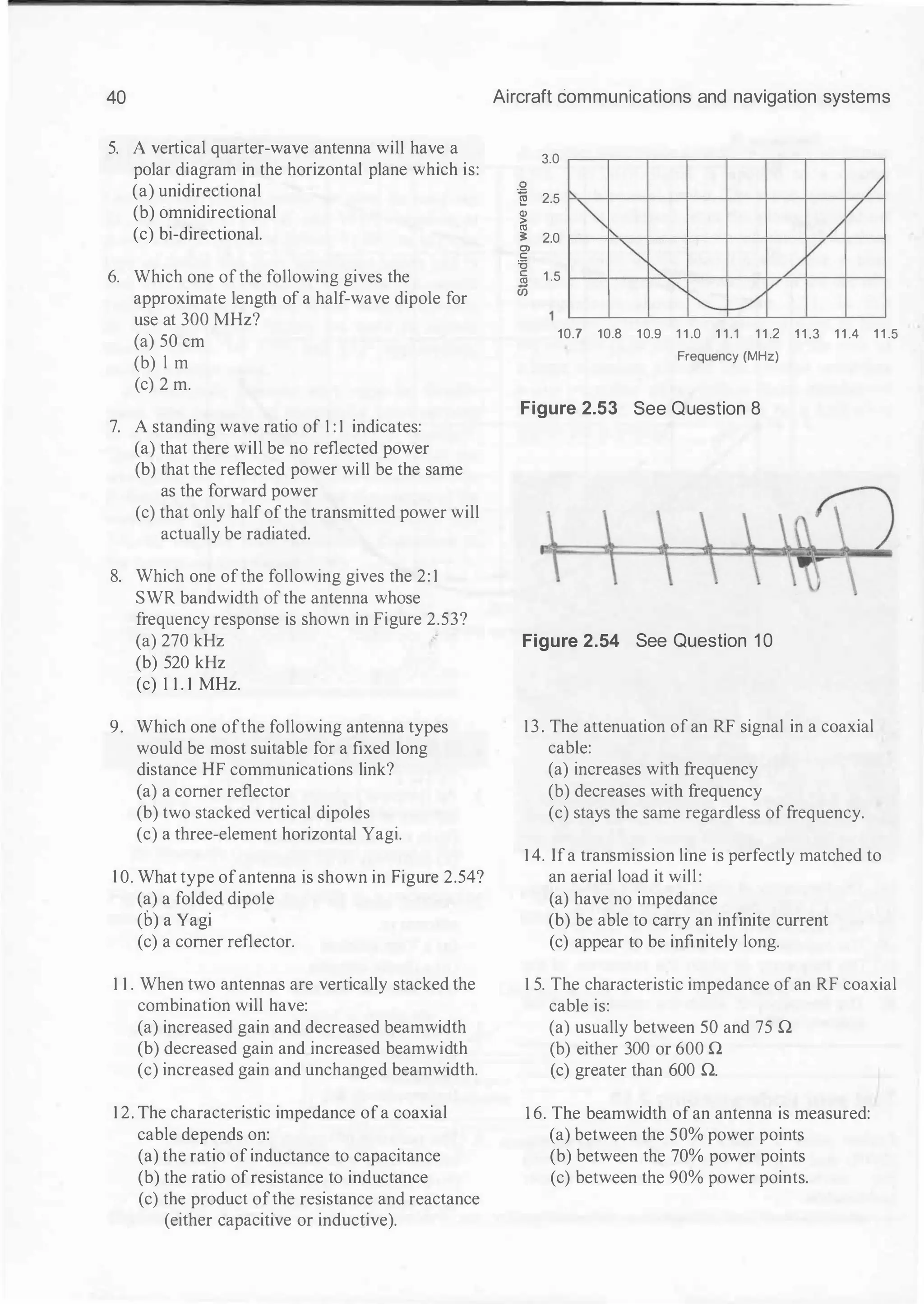
Figure 5.6 Examples of aircraft communication using HFDL
E
8
. . .](https://image.slidesharecdn.com/aircraftcommunicationsandnavigationsystemsprinciplesoperationandmaintenancepdfdrive-250205173033-c029e156/75/Aircraft-communications-and-navigation-systems_-principles-operation-and-maintenance-PDFDrive-pdf-88-2048.jpg)
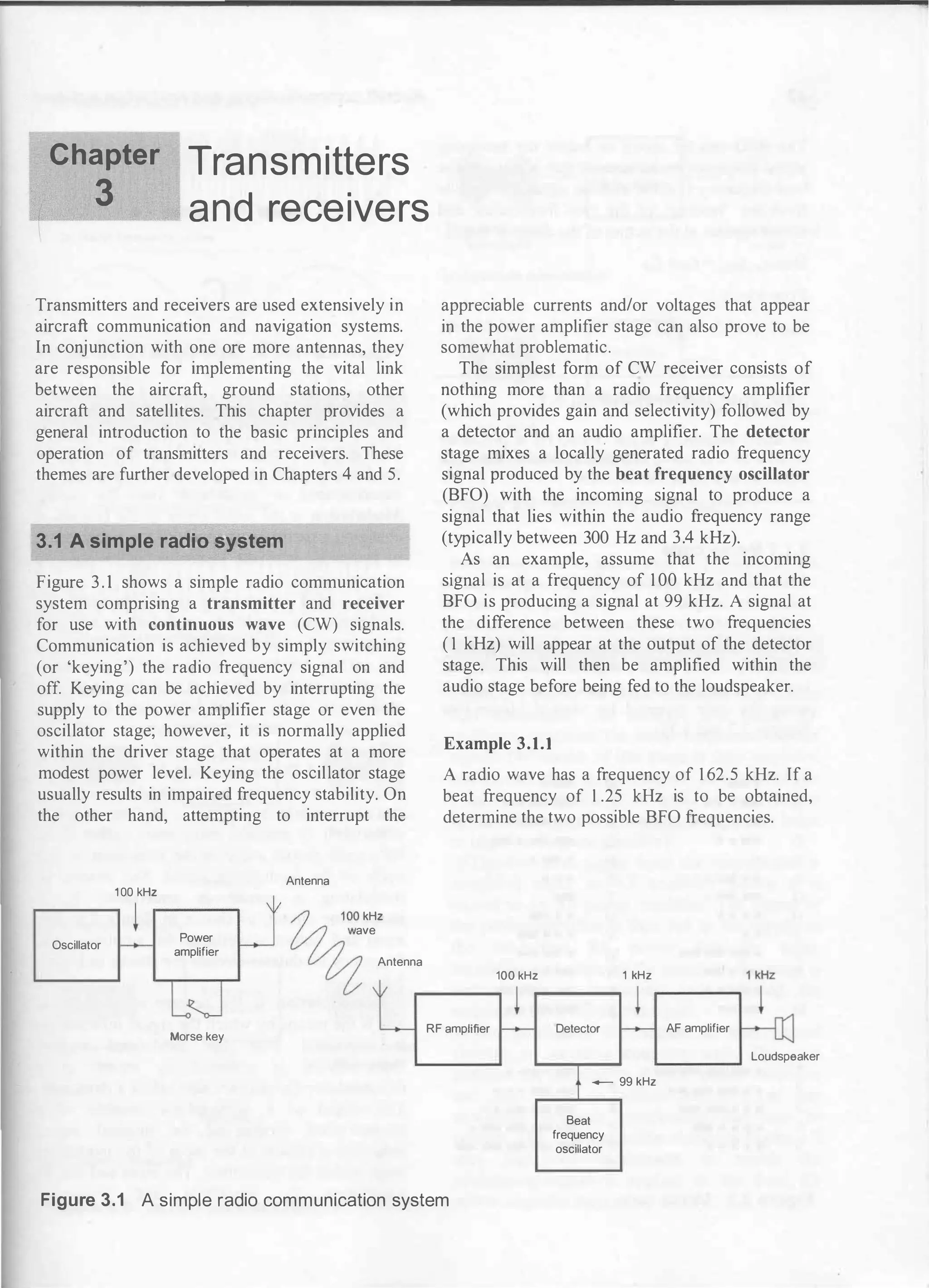
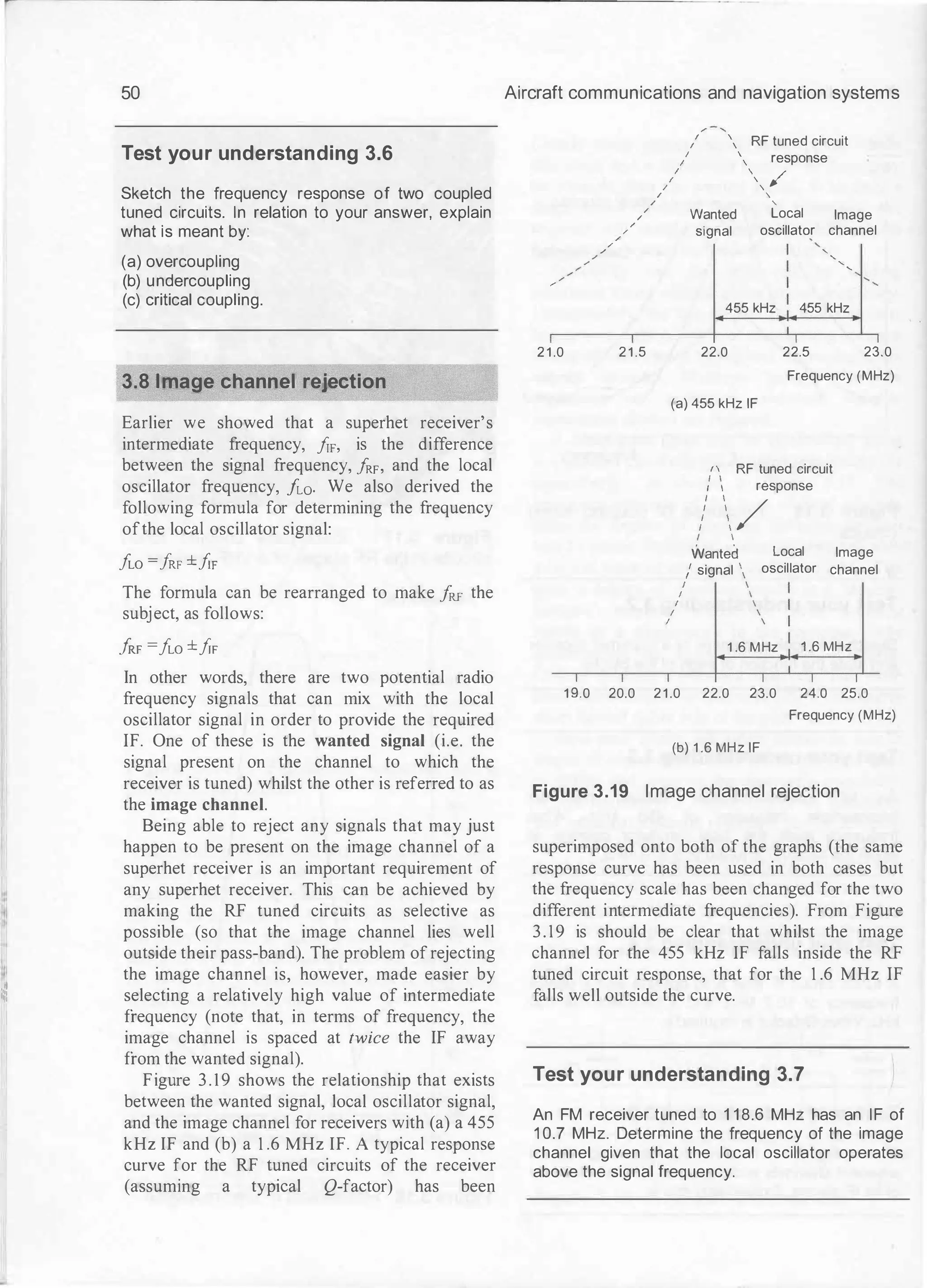
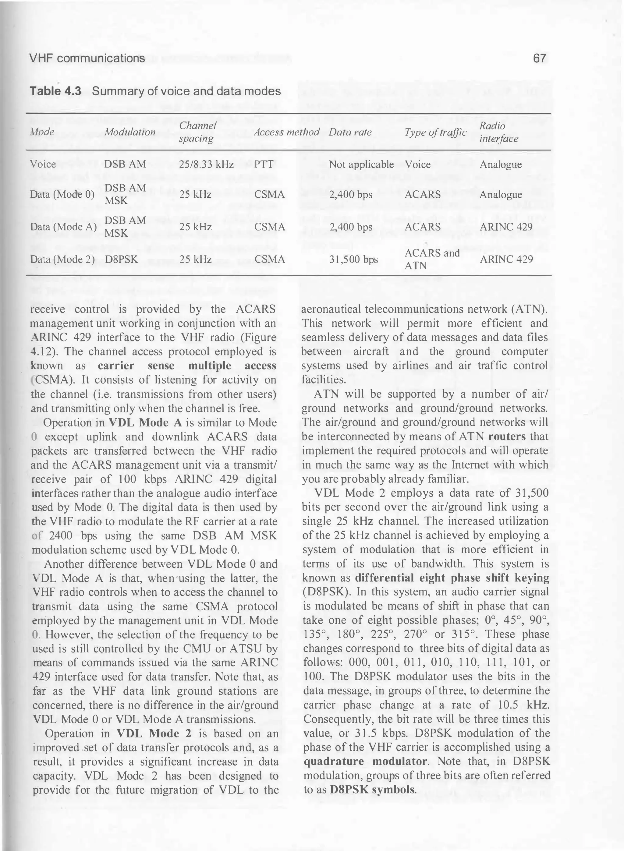
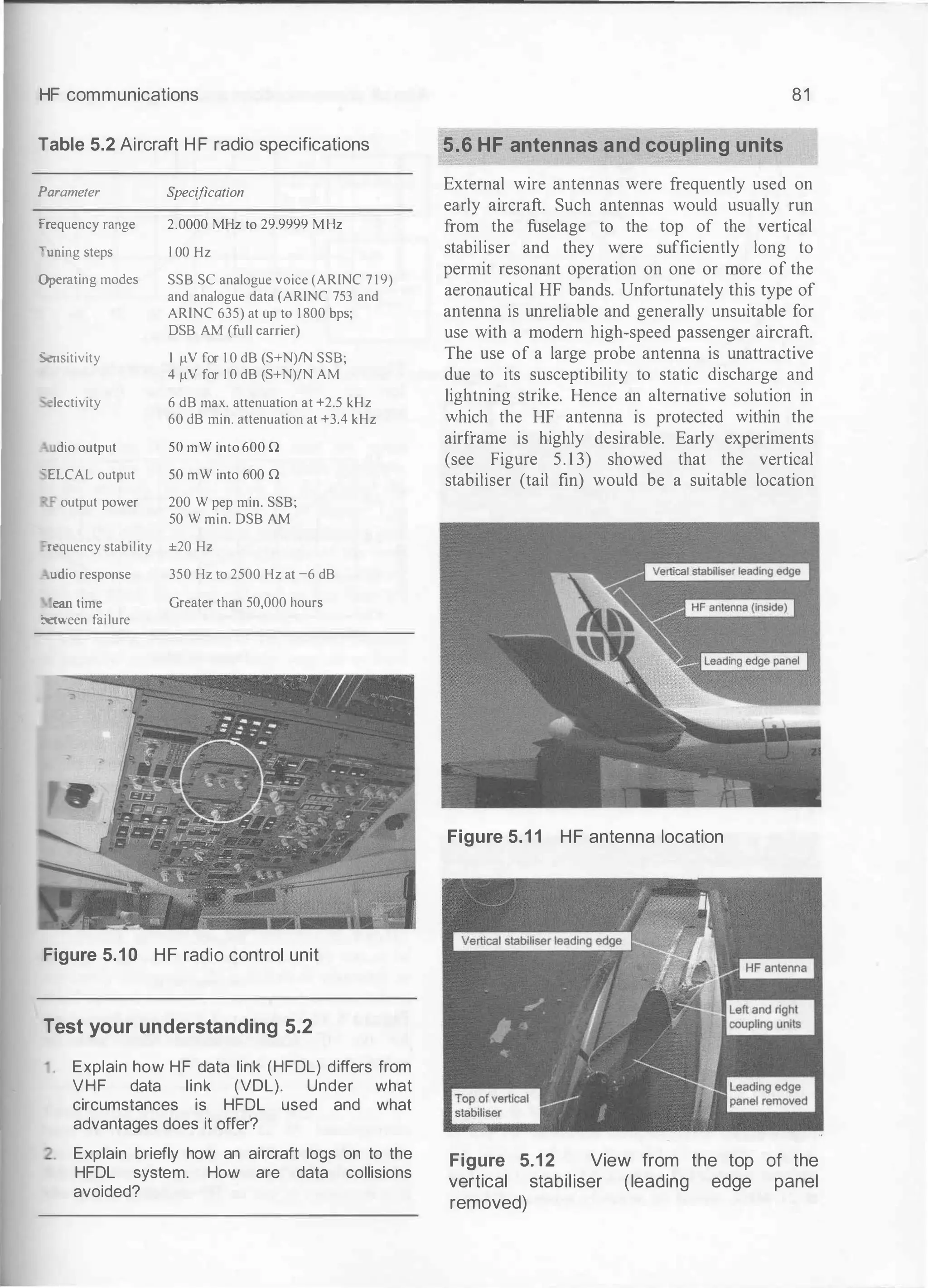
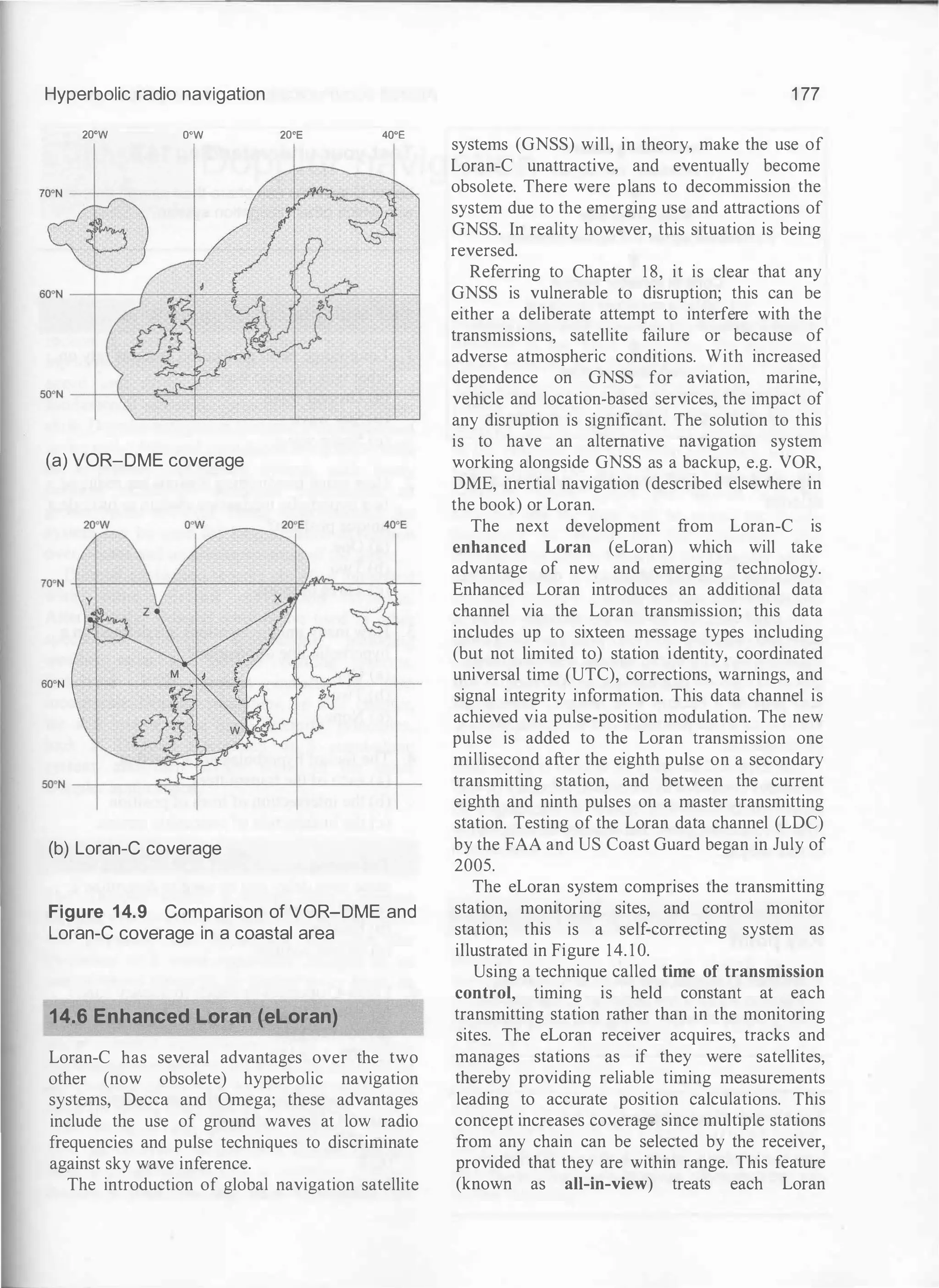
![80 Aircraft communications and navigation systems
5.5 HF radio equipment
The block schematic of a simple HF transmitter/
receiver is shown in Figure 5.9. Note that, whilst
this equipment uses a single intermediate
frequency (IF), in practice most modem aircraft
HF radios are much more complex and use two or
three intermediate frequencies.
On transmit mode, the DSB suppressed carrier
(Figure 5.2b) is produced by means of a
balanced modulator stage. The balanced
modulator rejects the carrier and its output just
comprises the upper and lower sidebands. The
DSB signal is then passed through a multiple
stage crystal or mechanical filter. This filter has a
very narrow pass-band (typically 3.4 kHz) at the
intermediate frequency (IF) and this rejects the
unwanted sideband. The resulting SSB signal is
then mixed with a signal from the digital
frequency synthesiser to produce a signal on the
wanted channel. The output from the mixer is
then further amplified before being passed to the
output stage. Note that, to avoid distortion, all of
the stages must operate in linear mode.
Microphone
(]--
Microphone
f-.-
Balanced
f-.- Filter
amplifier modulator
ntenna 1
L
t 1
Antenna
TransmiU
Carrier
1-+--- receive
coupler oscillator
switching
A
t
RF
1---- Mixer
preamplifier
Transmit/receive +
control -
Reference
oscillator
Figure 5.9 A simple SSB transmitter/receiver
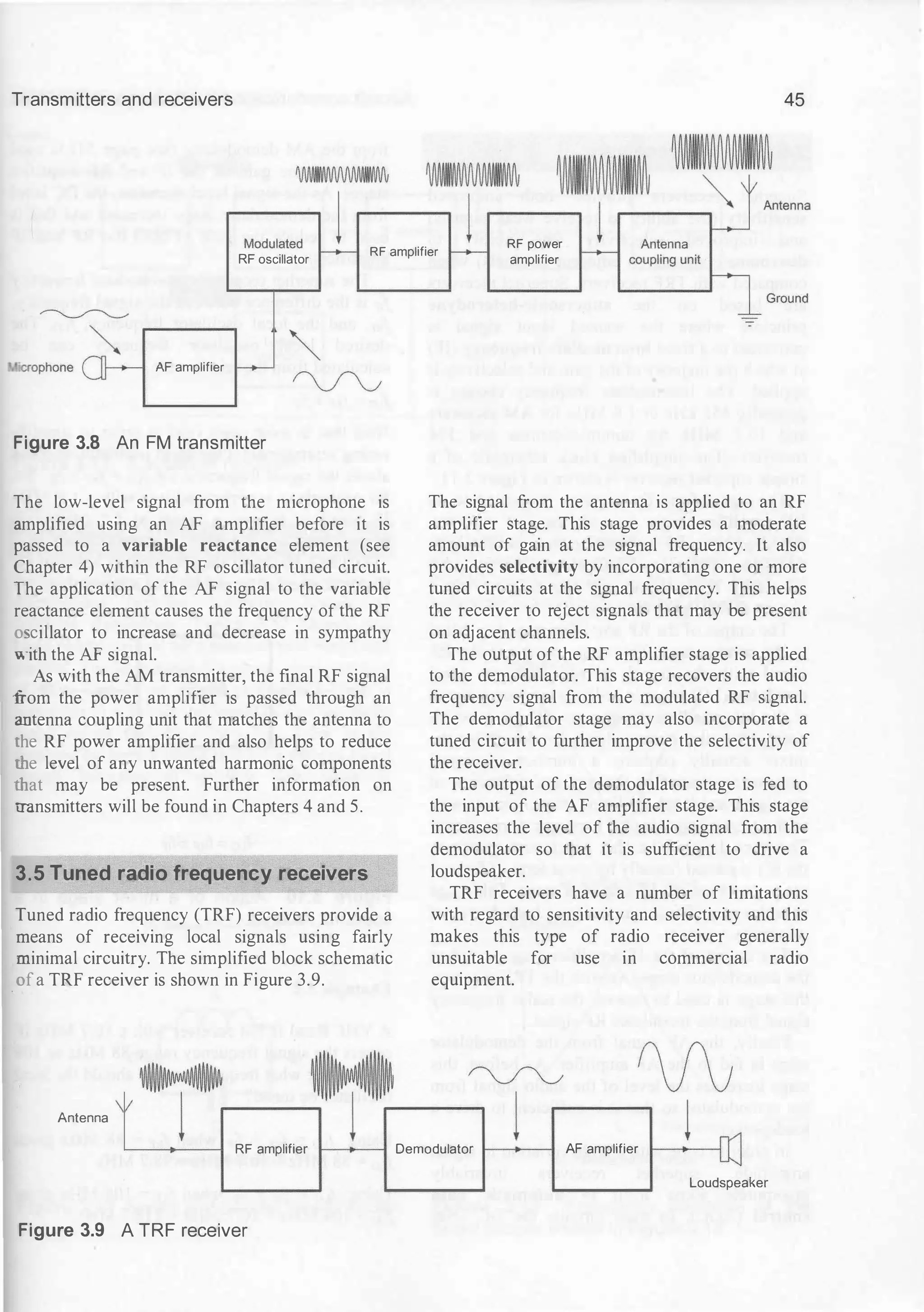
When used on receive mode, the incoming signal
frequency is mixed with the output from the
digital frequency synthesiser in order to produce
the intermediate frequency signal. Unwanted
adjacent channel signals are removed by means of
another multiple-stage crystal or mechanical filter
which has a pass-band similar to that used in the
transmitter. The IF signal is then amplified before
being passed to the demodulator.
The (missing) carrier is reinserted in the
demodulator stage. The carrier signal is derived
from an accurate crystal controlled carrier
oscillator which operates at the IF frequency. The
recovered audio signal from the demodulator is
then passed to the audio amplifier where it is
amplified to an appropriate level for passing to a
loudspeaker.
The typical specification for an aircraft HF
radio is shown in Table 5.2. One or two radios of
this type are usually fitted to a large commercial
aircraft (note that at least one HF radio is a
requirement for any aircraft following a trans
oceanic route). Figure 5.10 shows the flight deck
location ofthe HF radio controller.
f-.- Mixer f-.- f-.-
Power
I--
Driver
amplifier
!
r-oo
I-- f-.-
Audio
Demodulator
amplifier
Loudspeaker
+
t
1-+- Filter t--- IF amplifier
1-+- Digital frequency synthesiser
t u
Frequency control](https://image.slidesharecdn.com/aircraftcommunicationsandnavigationsystemsprinciplesoperationandmaintenancepdfdrive-250205173033-c029e156/75/Aircraft-communications-and-navigation-systems_-principles-operation-and-maintenance-PDFDrive-pdf-90-2048.jpg)
![86 Aircraft communications and navigation systems
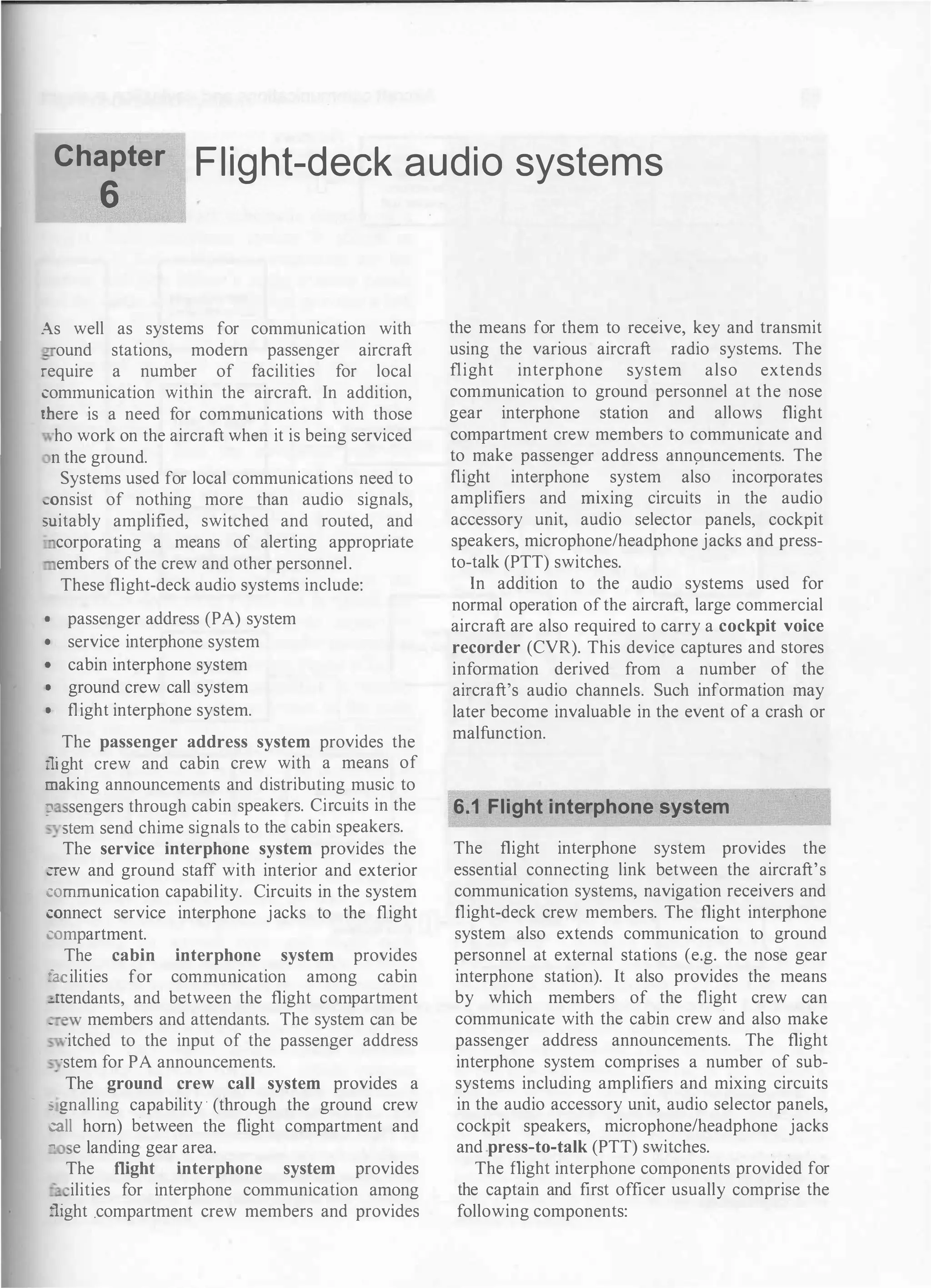
ptain's Firstofficer's
Ca
speaker
Captain's cockpit
Captain and First officer's speaker
co--
first officer's cockpit
�
interphone I+- audio selector f---- interphone
speaker unit
panels speaker unit
r- r--
Left VHF radio Right VHF radio
communications communications
Left HF radio Right HF radio - - - · ACARS
communications communications
I I
-
1
SELCAL unit
r
L__
Navigation Centre VHF radio
systems communications
-
Service
interphone jacks
Cockpit voice Electronic
recorder (CVR)
I
chimes
Cabin crew
Audio
Pilot's call Ground crew
--[1] Hom
handsets
accessory unit and
system call system
interphone amplifier
Audio
Passenger
� Cabin, toilet and cabin
reproducer
address (PA)
crew speakers
amplifier
Figure 6.1 Simplified block schematic diagram of a typical flight interphone system
• audio selector panel
• headset, headphone, and hand microphone
jack connectors
• audio selector panel and control wheel press
to-talk (PTT) switches
• cockpit speakers.
Note that, where a third (or fourth) seat is
provided on the flight deck, a third (or fourth) set
of flight interphone components will usually be
available for the observer(s) to use. In common
with other communication systems fitted to the
aircraft, the flight interphone system normally](https://image.slidesharecdn.com/aircraftcommunicationsandnavigationsystemsprinciplesoperationandmaintenancepdfdrive-250205173033-c029e156/75/Aircraft-communications-and-navigation-systems_-principles-operation-and-maintenance-PDFDrive-pdf-96-2048.jpg)
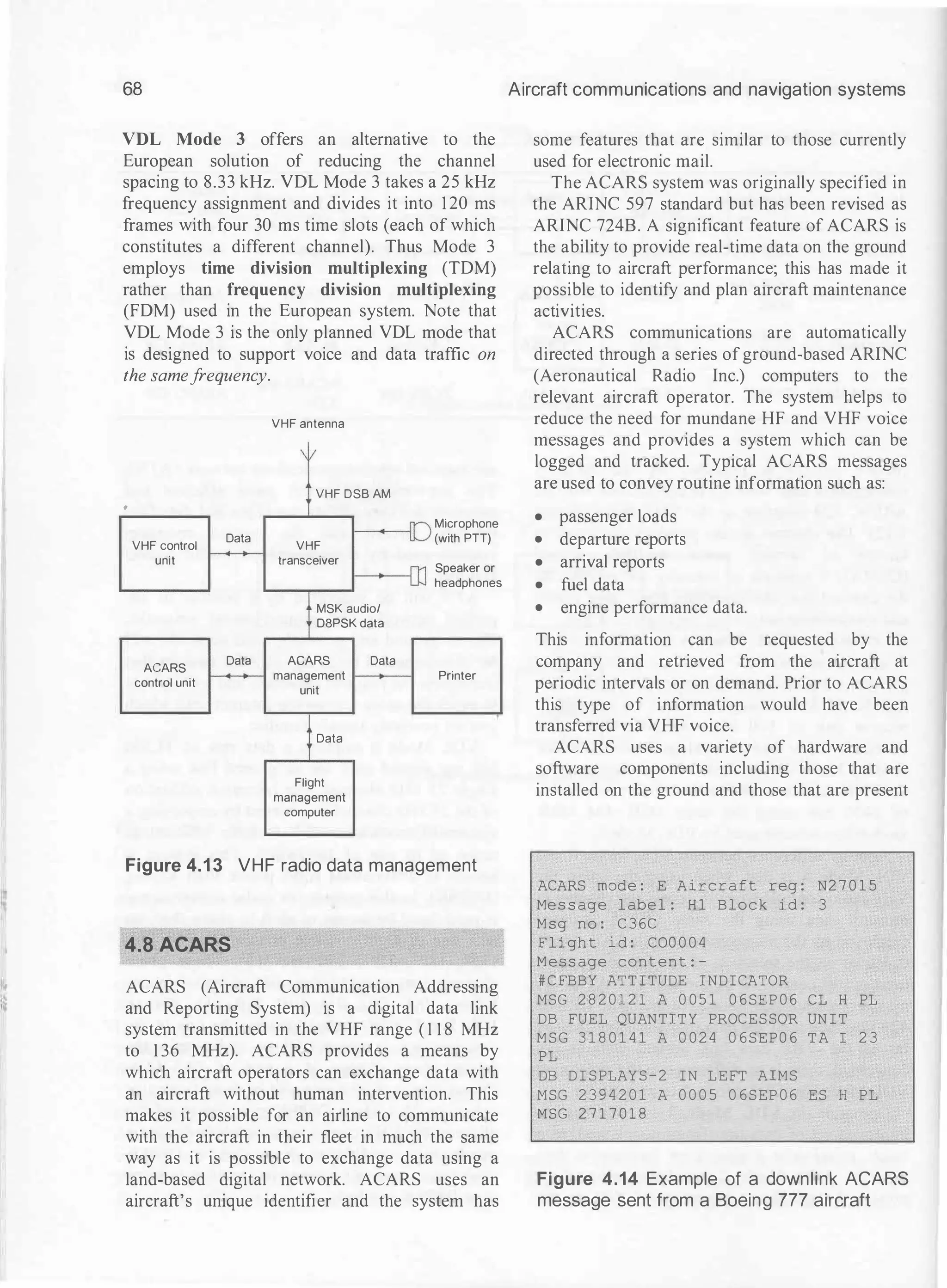
![88 Aircraft communications and navigation systems
Captain's control wheel
Audio
�PTT
Captain's headset
�
Boom microphone
®PTT
� Captain's
L interphone
s oxygen
�
Hand microphone l
I speaker
mask Oxygen mask t
Noise reduction
Captain'
HFNHF radio {
communications
microphone
m m rni] m [l�H!ll lOOJ }HFNHF radio
communications
equipment,
interphone audio
PA and CVR
$ $ $ $ 8 8 8
equipment,
navigation and
interphone audio
8_$ Q�Q
• Q ••a
$�$
� � ll �
Captain's audio selector panel
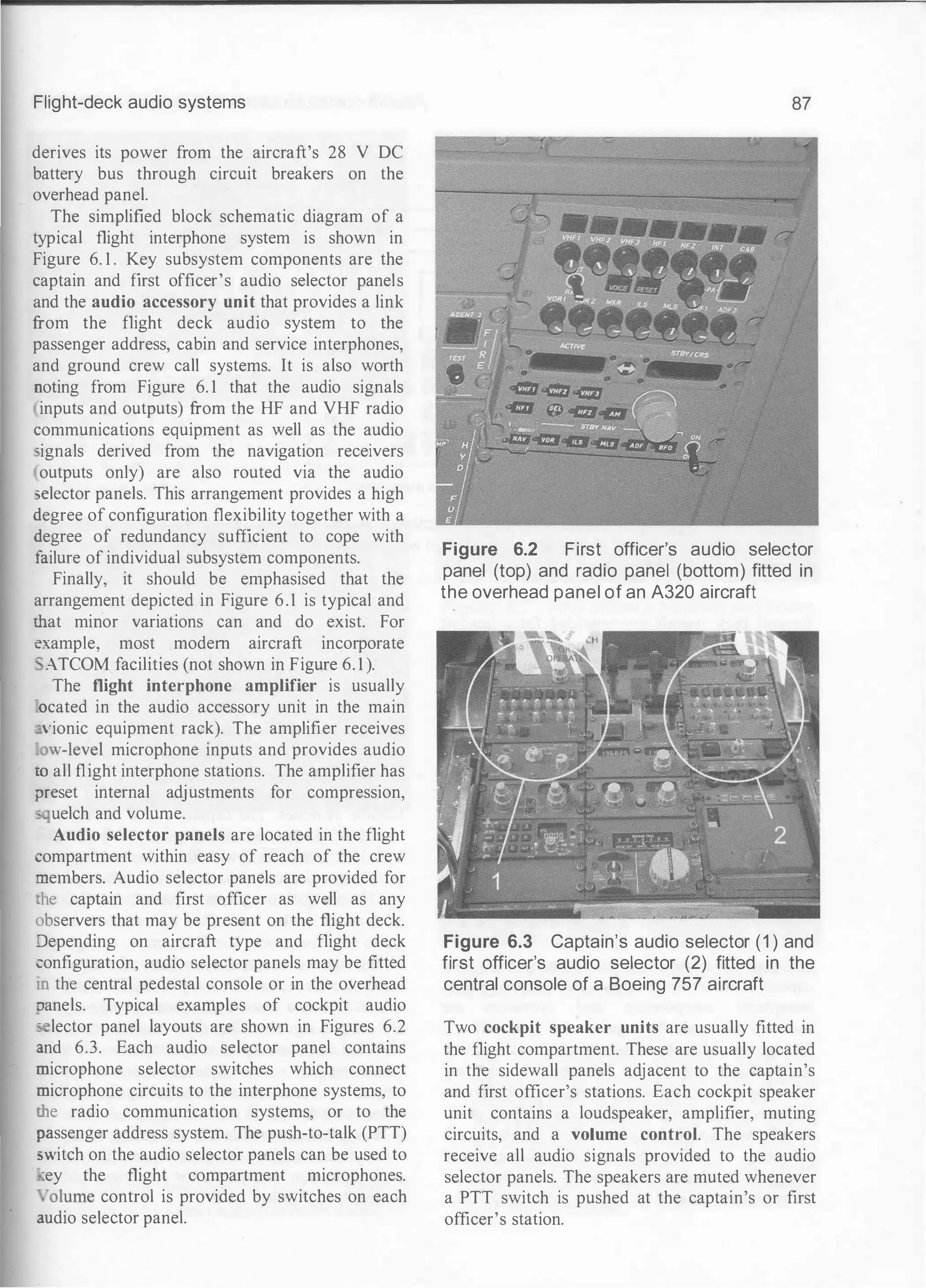
Figure 6.4 Typical arrangement for the captain's audio selector. A similar arrangement is
used for the first officer's audio selector as well as any supernumerary crew members that ma
be present on the flight deck
Several jack panels are provided for a headset
with integral boom microphone for the captain,
first officer and observer. Hand microphones
may also be used. Push-to-talk (PTT) switches
are located at all flight interphone stations. The
hand microphone, control wheel, and audio
selector panels all have PTT switches. The switch
must be pushed before messages are begun or no
transmission can take place. Audio and control
circuits to the audio selector panel are completed
when the PTT switch is operated.
The flight interphone system provides common
microphone circuits for the communications
systems and common headphone and speaker
circuits for the communications and navigation
systems.
Figure 6.4 shows a typical arrangement for the
captain's audio selector panel (note that the flight
interphone components and operation are
identical for both the captain and first officer).
Similar (though not necessarily identical) systems
are available for use by the observer and any
other supernumerary crew members (one obvious
difference is the absence of a control wheel push
to-talk switch and cockpit speaker). Switches are
provided to select boom microphone, hand
microphone (where available) as well as
microphones located in the oxygen masks (for
emergency use). Outputs can be selected for use
with the headset or cockpit loudspeakers.
Amplifiers, summing networks, and filters iL
the audio selector panel provide audio signals
from the interphone and radio communicatio
systems to the headphones and speakers. Audio
signals from the navigation receivers are also
monitored through the headphones and speakers
Reception of all audio signals is controlled by the
volume switches. The captain's INT microphone
switch is illuminated when active. Note that this
switch is interlocked with the other microphone
switches so that only one at a time can be pushed.
The navigation system's (ADF, VOR, IL
etc.) audio is also controlled by switches on the
audio selector panel. The left, centre, or right (L
C, R) switches control selection and volume o:
the desired receiver. The VOICE-BOTH-RANGE
switch acts as a filter that separates voice signals
and range signals. The filter switch can alsc
combine both voice and range signals. All radi
communication, interphone, and navigatio
outputs are received and recorded by the cockpit
voice recorder (CVR).
A typical procedure for checking that th
microphone audio is routed to the radic
communication, interphone, or passenger address
system is as follows:](https://image.slidesharecdn.com/aircraftcommunicationsandnavigationsystemsprinciplesoperationandmaintenancepdfdrive-250205173033-c029e156/75/Aircraft-communications-and-navigation-systems_-principles-operation-and-maintenance-PDFDrive-pdf-98-2048.jpg)
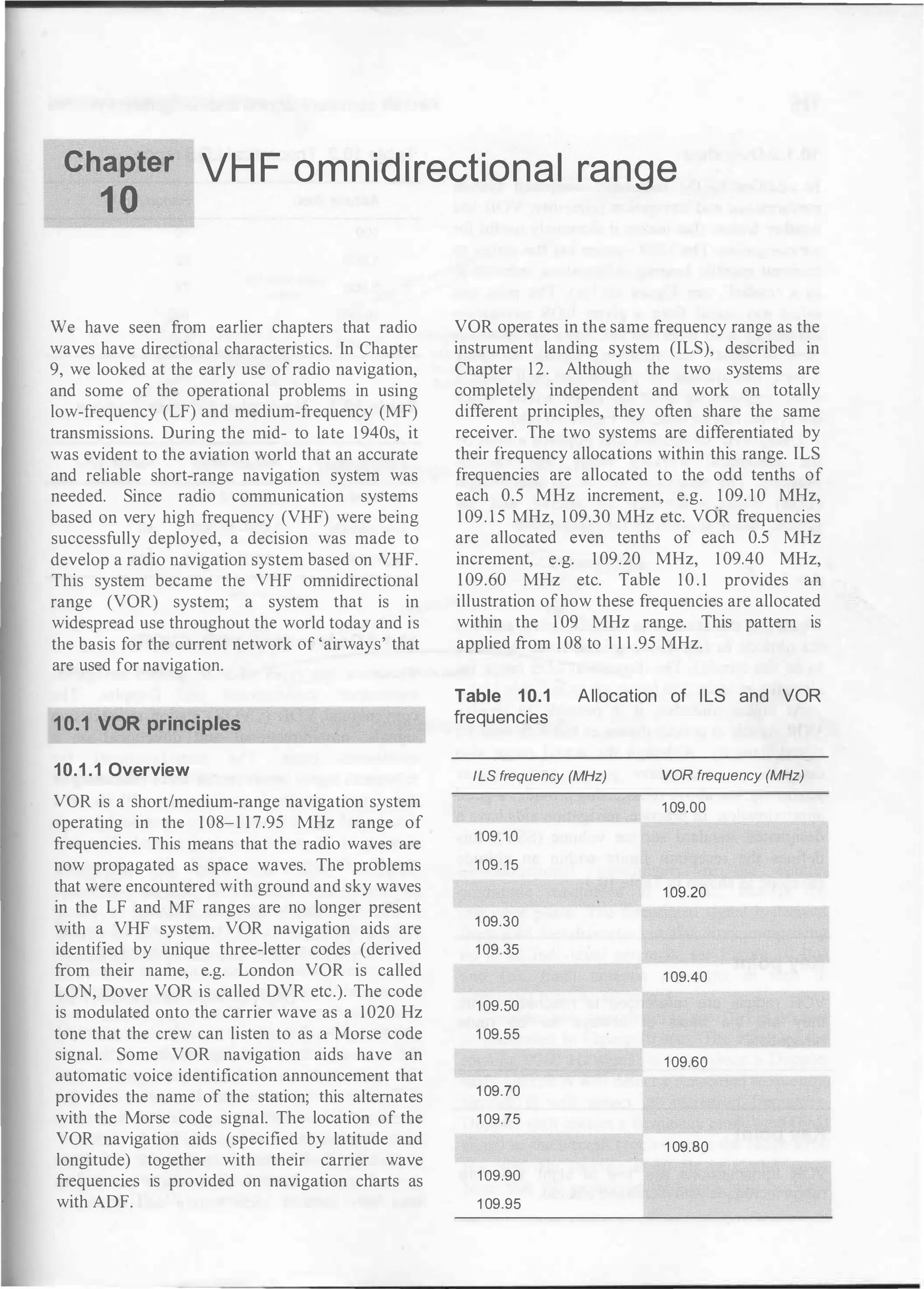
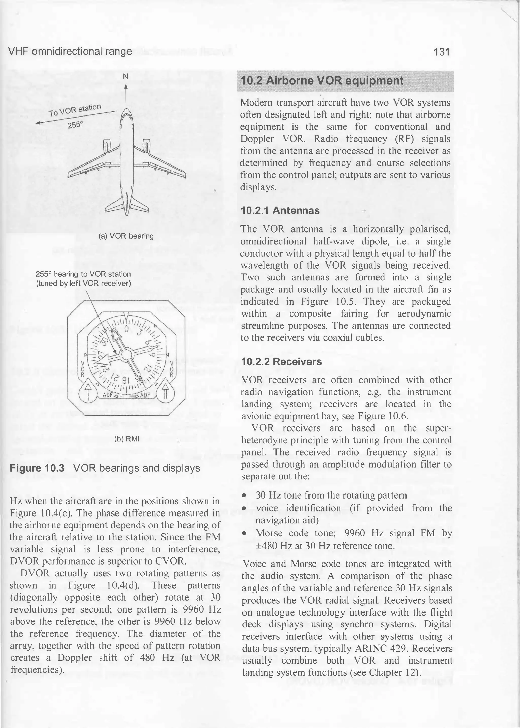
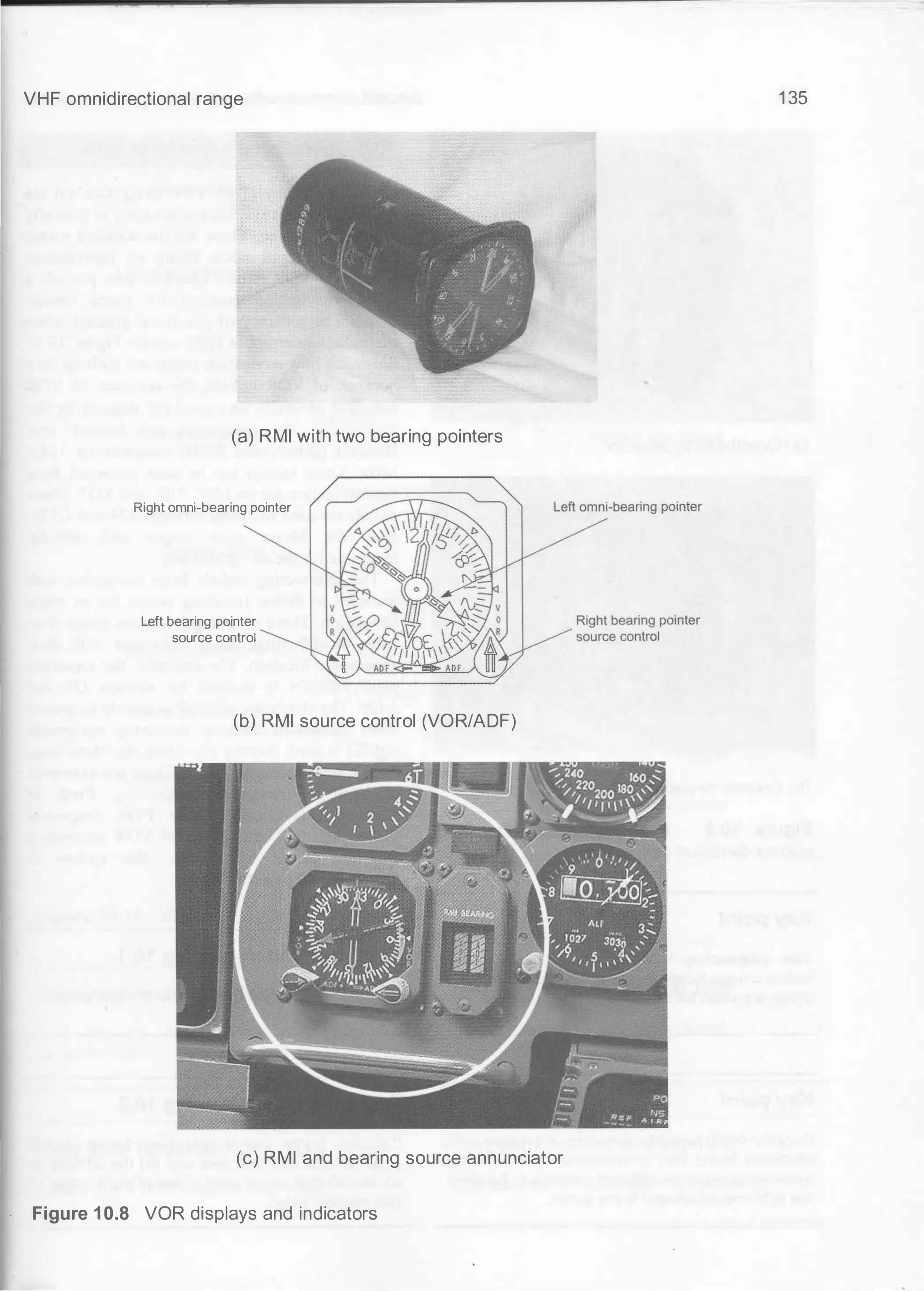
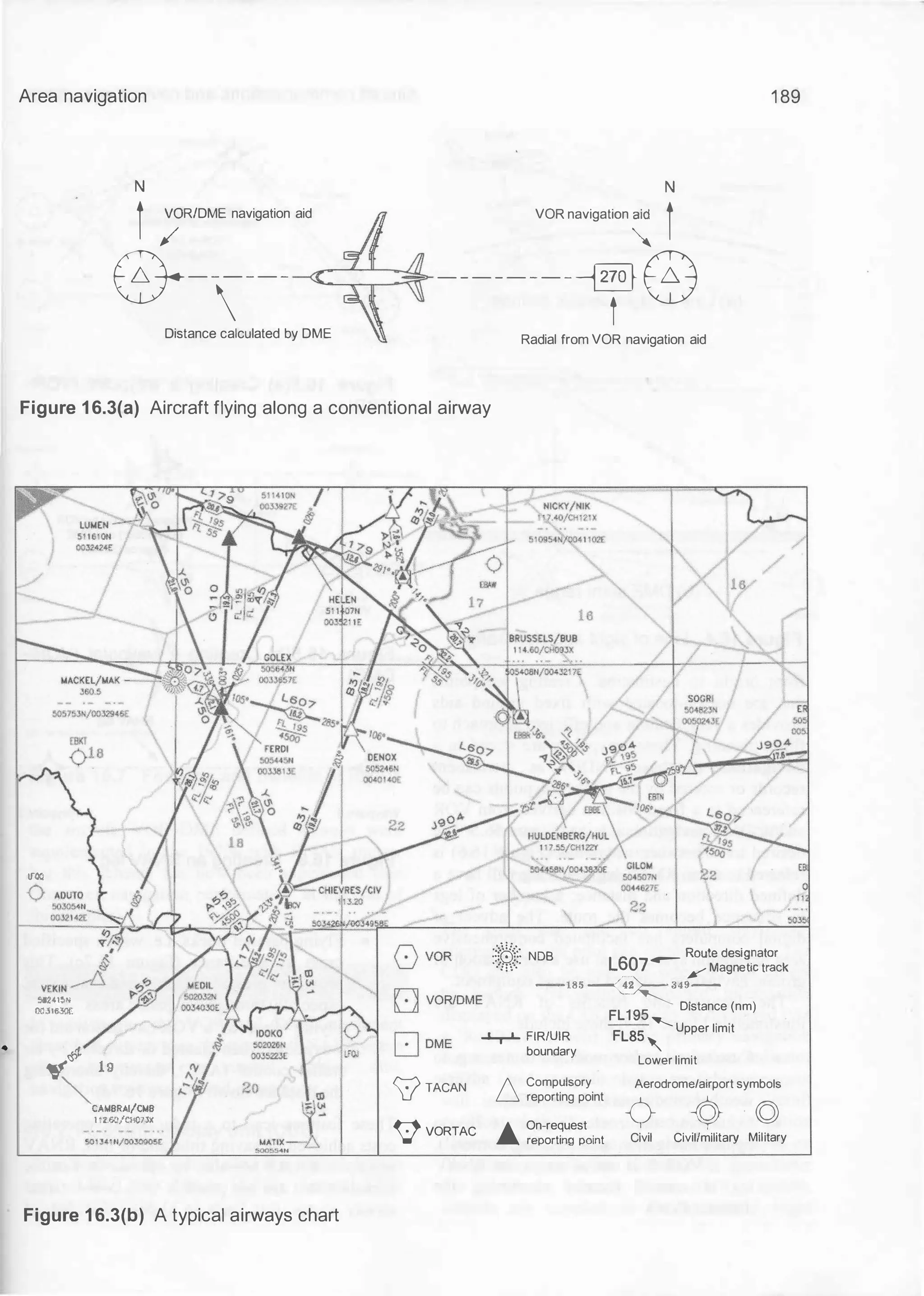
![VHF omnidirectional range
lfllQ
0
�
�<:s 19
�CAWBRAI/CioiB
ll2.ISO/CH07JX
50134tN/OOJ0905£
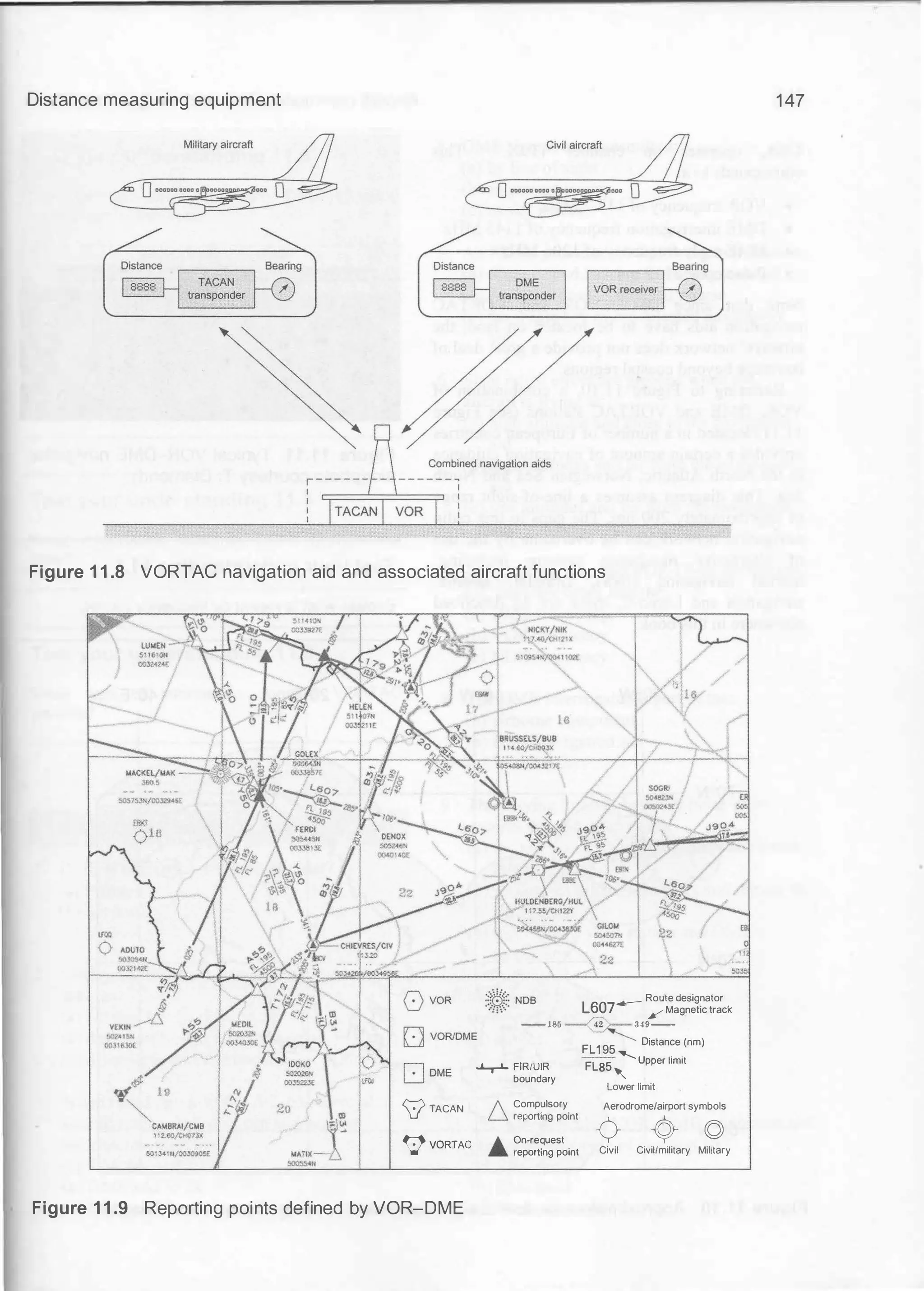
D oME
V TACAN
9voRTAC
NIC�Y/NI�
•
].<0/0<'2X
:(1�i!: NOB
-- 185
� FIR/UIR
boundary
1 Compulsory
U reporting point
"- On-request
A reporting point
1 39
22
� Route designator
L607 Magnetic
349� bearing
FL195
Distance (nm)
FLBS
......._
Upper limit
'
Lower limit
Aerodrome/airport symbols
-c) � (Q)
Civil Civil/military Military
(c) Airway network over Belgium
Figure 10.11 (continued)
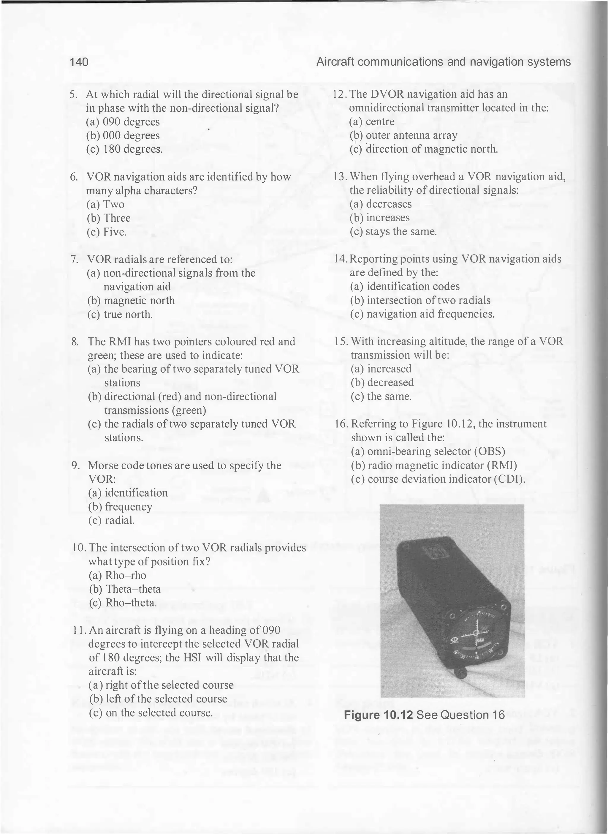
10.4 Multiple choice questions
1 . VOR operates in which frequency range?
(a) LF
(b) MF
(c) VHF.
2. VOR signals are transmitted as what type of
wave?
(a) Sky wave
(b) Ground wave
(c) Space wave.
3. Where is the deviation from a selected VOR
radial displayed?
(a) RMI
(b) HSI
(c) NDB.
4. At which radial will the directional wave be
out ofphase by 90 degrees with the non
directional wave?
(a) 090 degrees
(b) 000 degrees
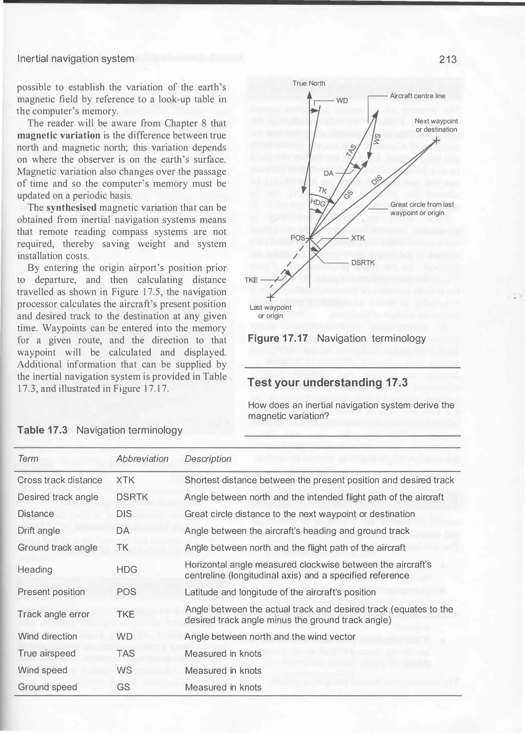
(c) 1 80 degrees.](https://image.slidesharecdn.com/aircraftcommunicationsandnavigationsystemsprinciplesoperationandmaintenancepdfdrive-250205173033-c029e156/75/Aircraft-communications-and-navigation-systems_-principles-operation-and-maintenance-PDFDrive-pdf-149-2048.jpg)
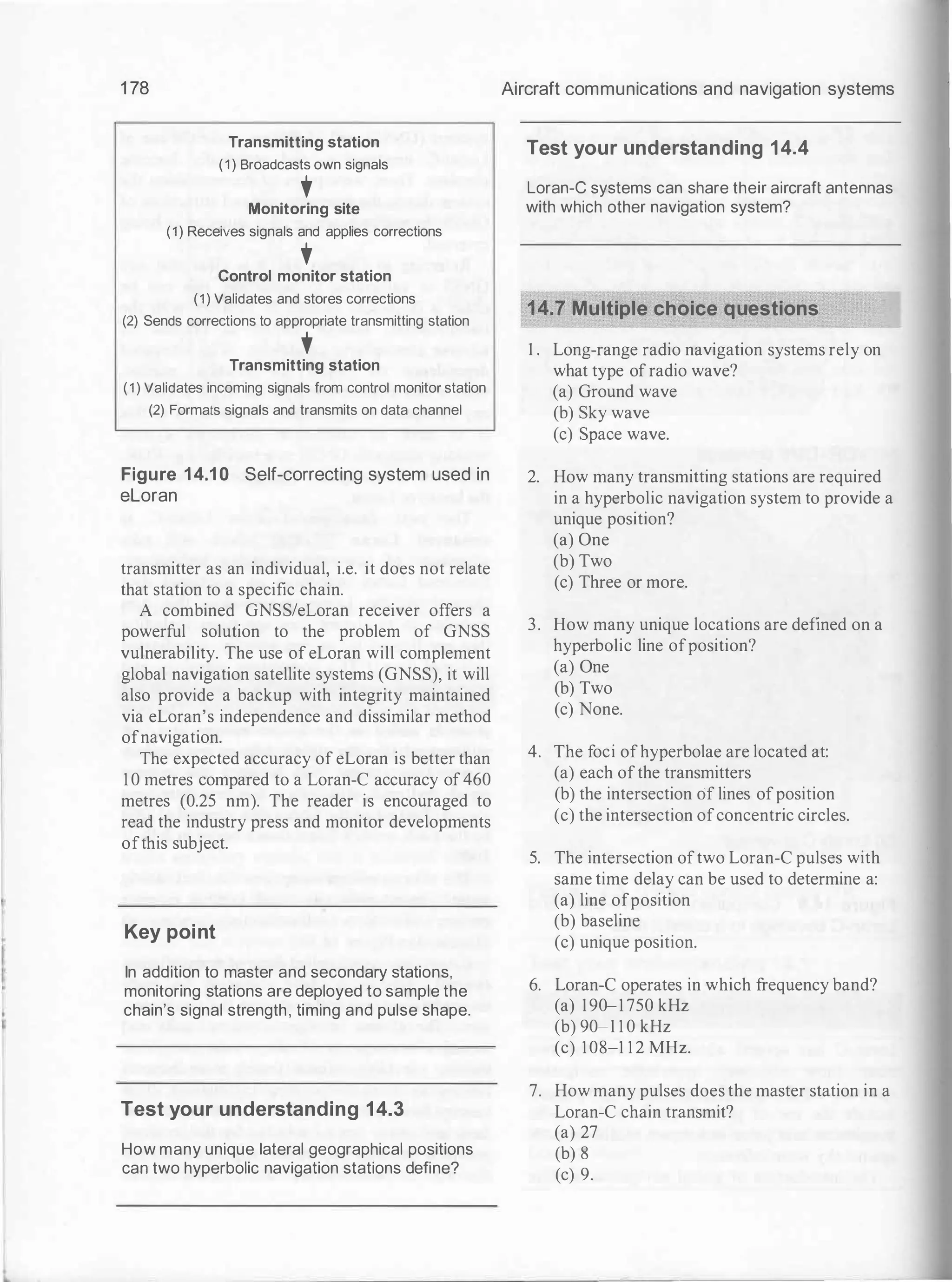
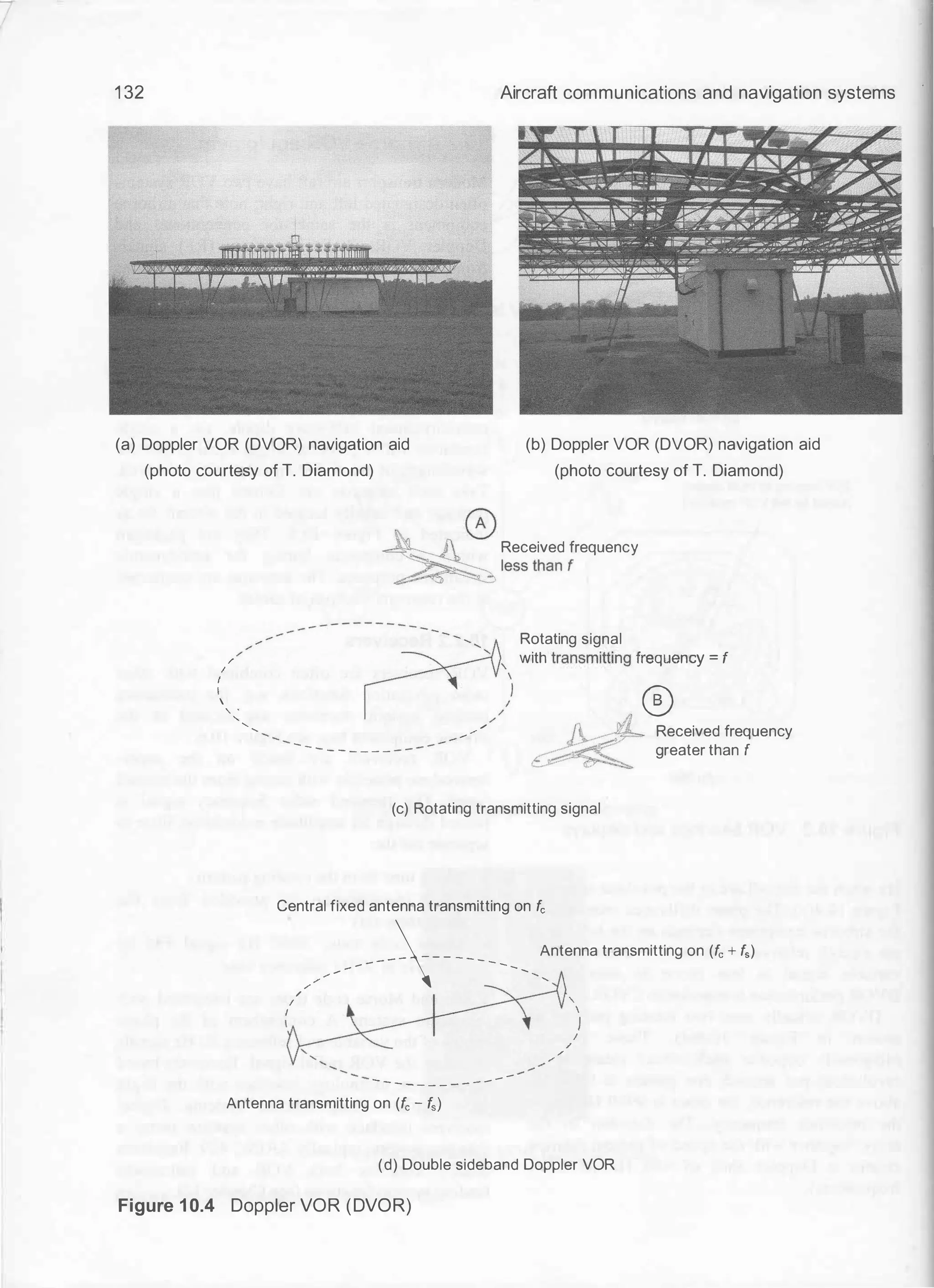
![1 80
�-
Observer
{a) Train moving towards the observer (more cycles in a given time
therefore the observer perceives a higher pitch)
��
•
Observer
(b) Train nearest to the observer {observer perceives the exact pitch)
l••••••(l•• ':"
. _
{ :._]
- �
Observer
(c) Train moving away from the observer {less cycles in a given
time therefore the observer perceives a lower pitch)
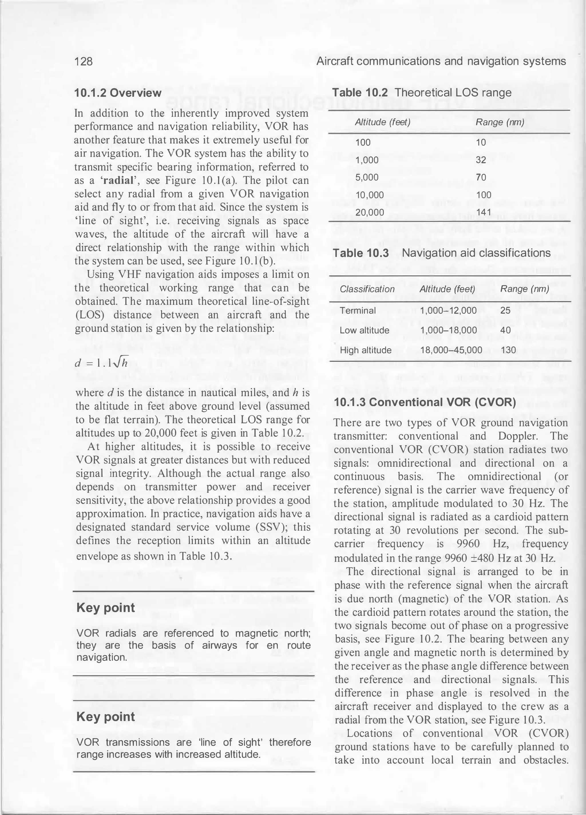
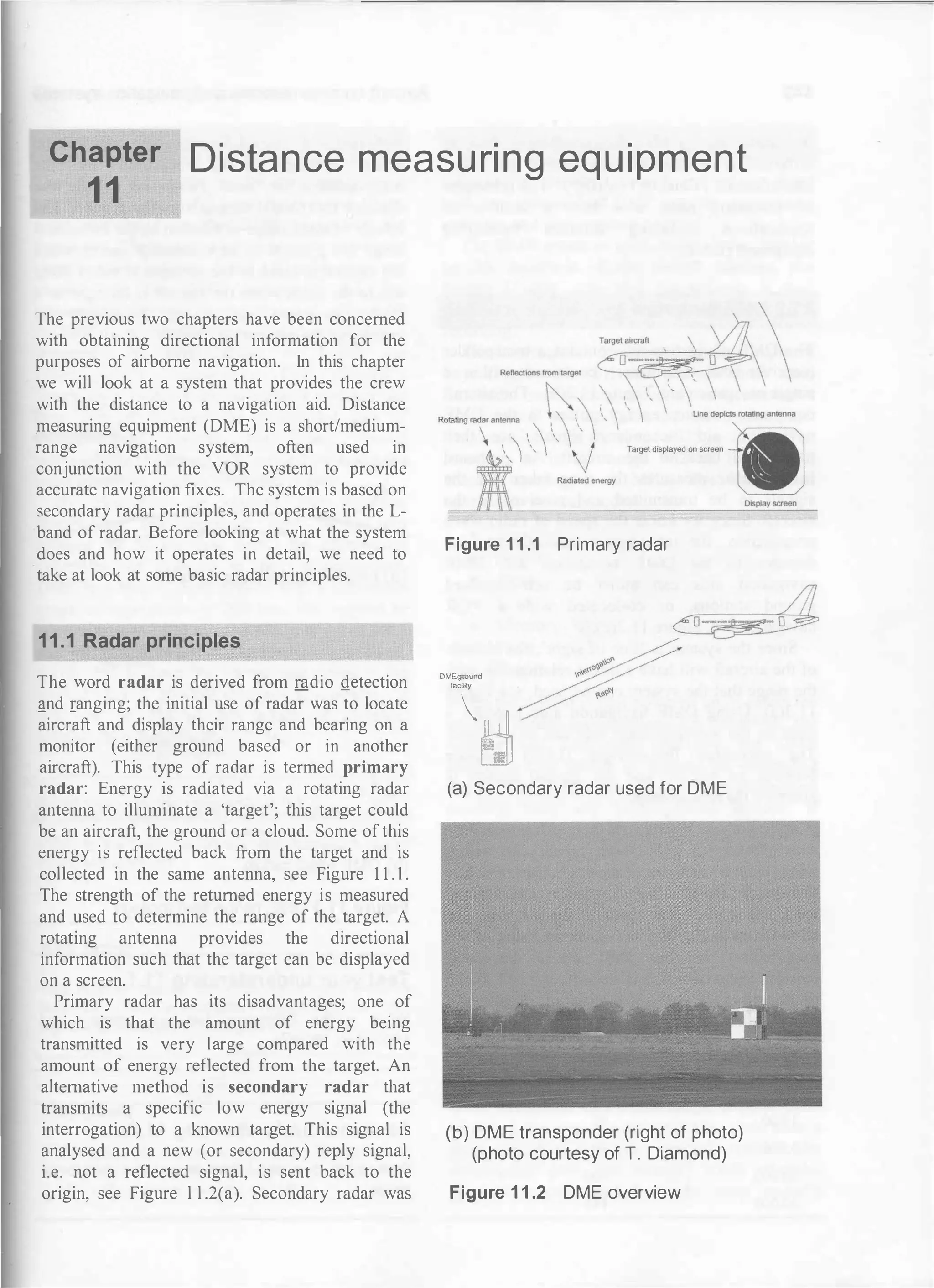
Figure 1 5.1 The Doppler effect
(a) Beamtransmitted ahead
of aircraft
Figure 1 5.2 Doppler navigation principles
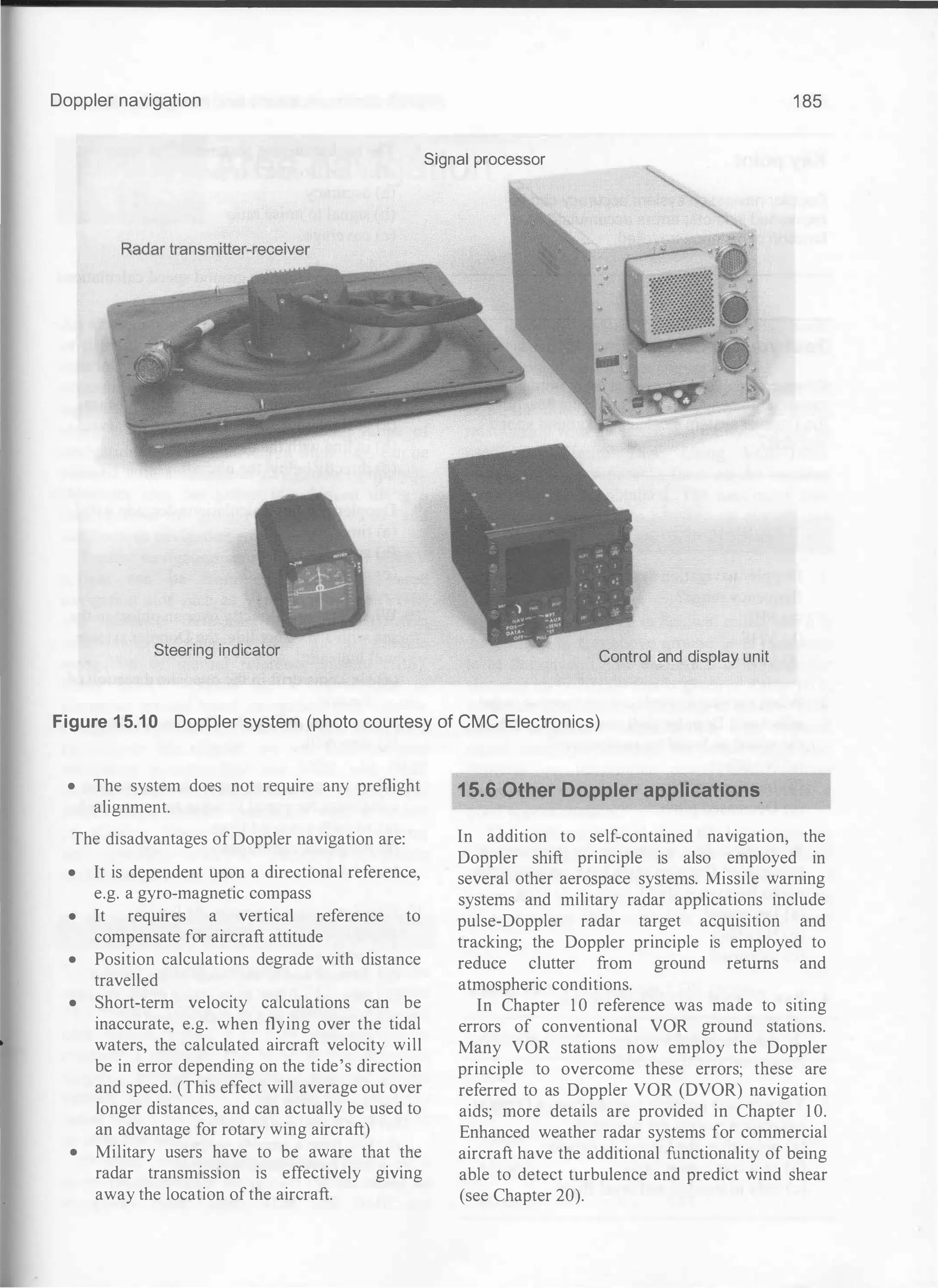
Aircraft communications and navigation systems
• Aircraft range to the terrain
• Backscattering features ofthe terrain
• Atmospheric conditions, i.e. attenuation
and absorption ofradar energy
• Radar equipment.
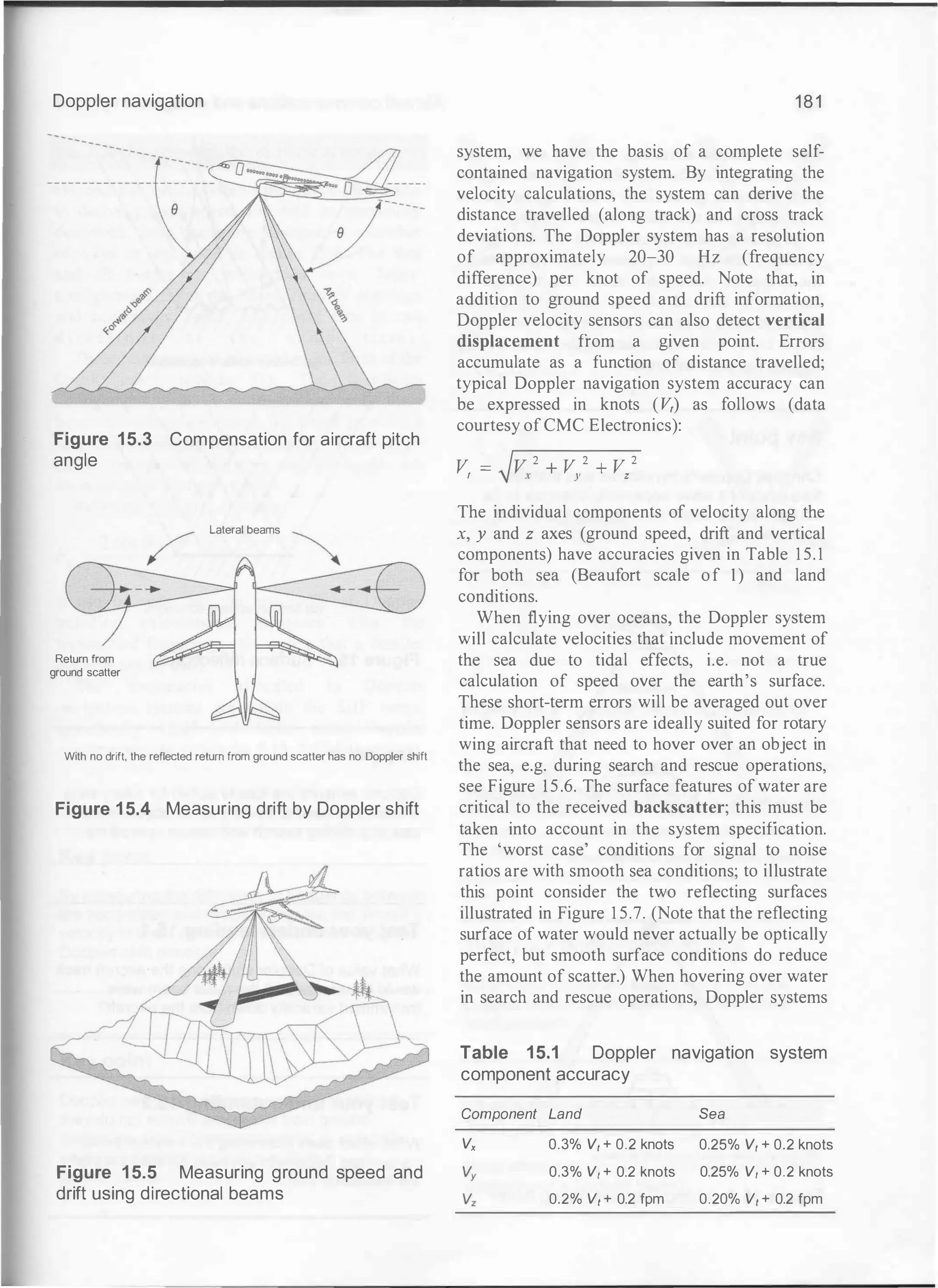
Note that the aircraft in Figure 15.2 is flying
straight and level. If the aircraft were pitched up
or down, this would change the angle ofthe beam
with respect to the aircraft and the surface; this
will change the value of Doppler shift for a given
ground speed. This situation can be overcome in
one of two ways; the transmitter and receiver can
be mounted on a stabilised platform or (more
usually) two beams can be transmitted from the
aircraft (forward and aft) as shown in Figure 15.3.
By comparing the Doppler shift of both beams, a
true value of ground speed can be derived. The
relationship between the difference in frequencies
and velocity in an aircraft can be expressed as:
F. _ 2 cos B x v
f
D -
C
where FD = frequency difference, e = the angle
between the beam and aircraft, v = aircraft
velocity, f = frequency of transmission, and c =
Speed of electromagnetic propagation (3 X 10�
metres/second).
Note that a factor of two is needed in the
expression since both the transmitter and receiver
are moving with respect to the earth's surface. It
can be seen from this expression that aircraft
altitude is not a factor in the basic Doppler
calculation. Modem Doppler systems (such as the
CMC Electronics fifth generation system) operate
up to 1 5,000 feet (rotary wing) and 50,000 feet
(fixed wing).
Having measured velocity along the track of
the aircraft, we now need to calculate drift. This
can be achieved by directing a beam at right
angles to the direction of travel, see Figure 15.4.
Calculation of drift is achieved by utilising the
same principles as described above. In practical
installations, several directional beams are used.
see Figure 1 5.5.
The calculation of ground speed and drift
provides 'raw navigation' information. By
combining these two values with directional
information from a gyro-magnetic compass](https://image.slidesharecdn.com/aircraftcommunicationsandnavigationsystemsprinciplesoperationandmaintenancepdfdrive-250205173033-c029e156/75/Aircraft-communications-and-navigation-systems_-principles-operation-and-maintenance-PDFDrive-pdf-190-2048.jpg)
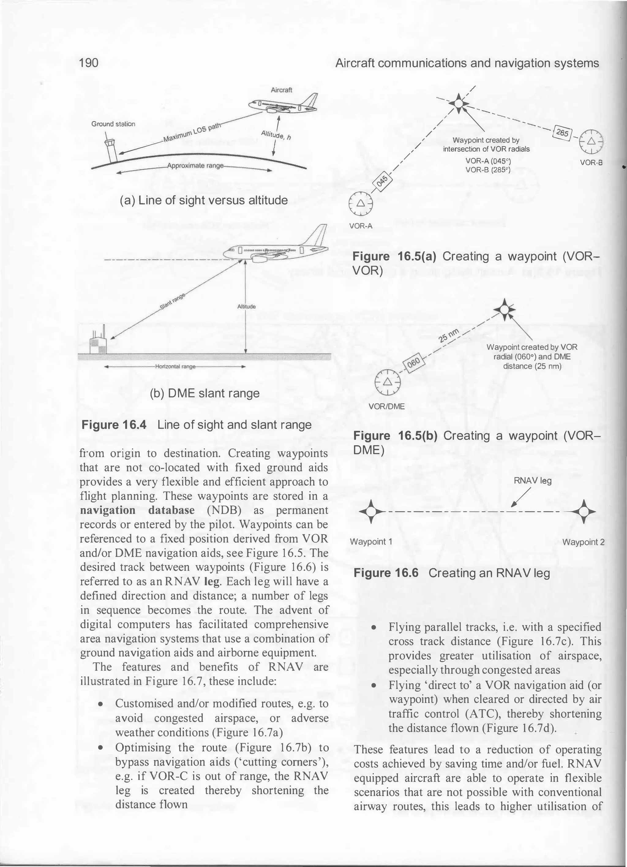
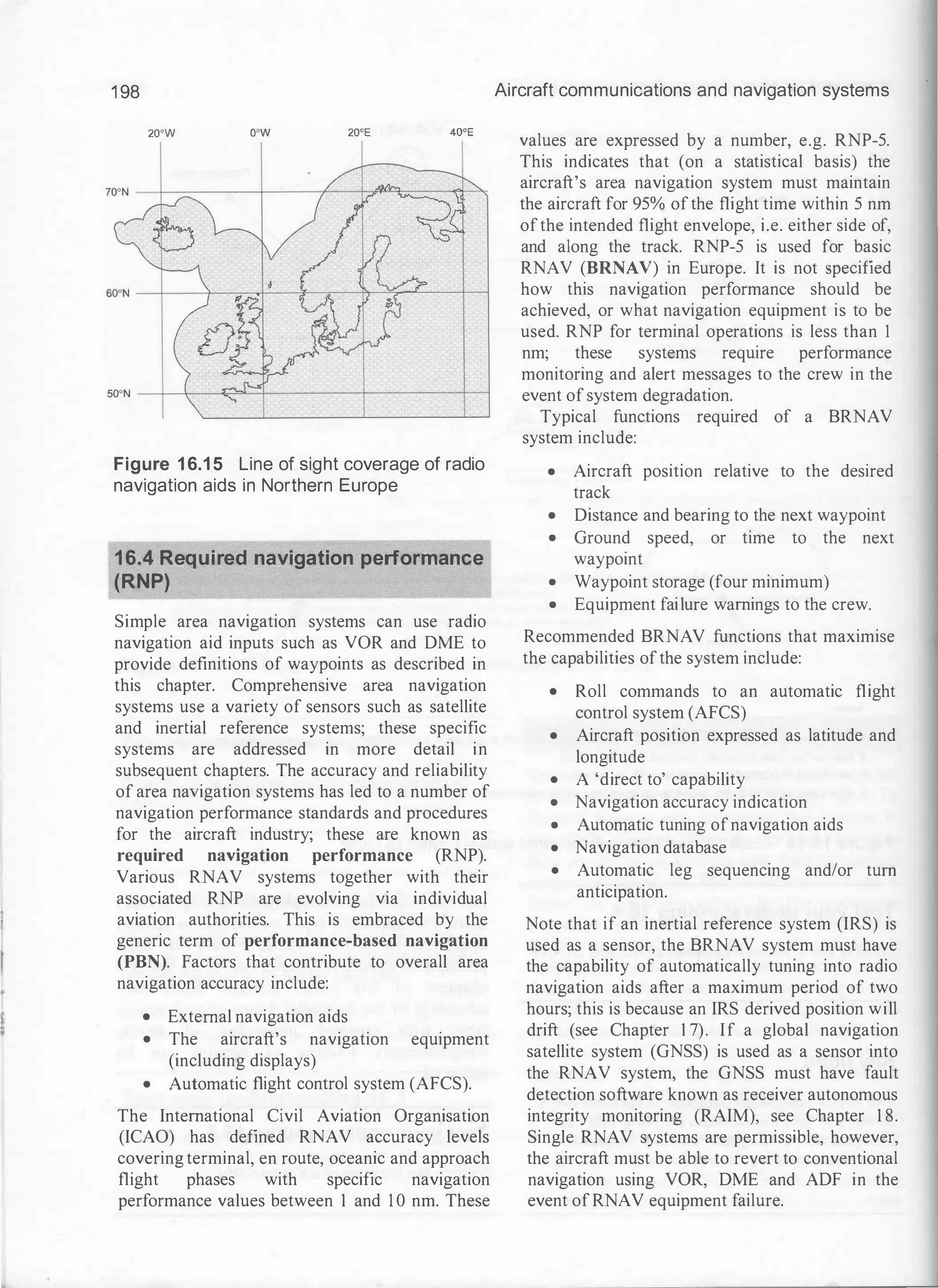
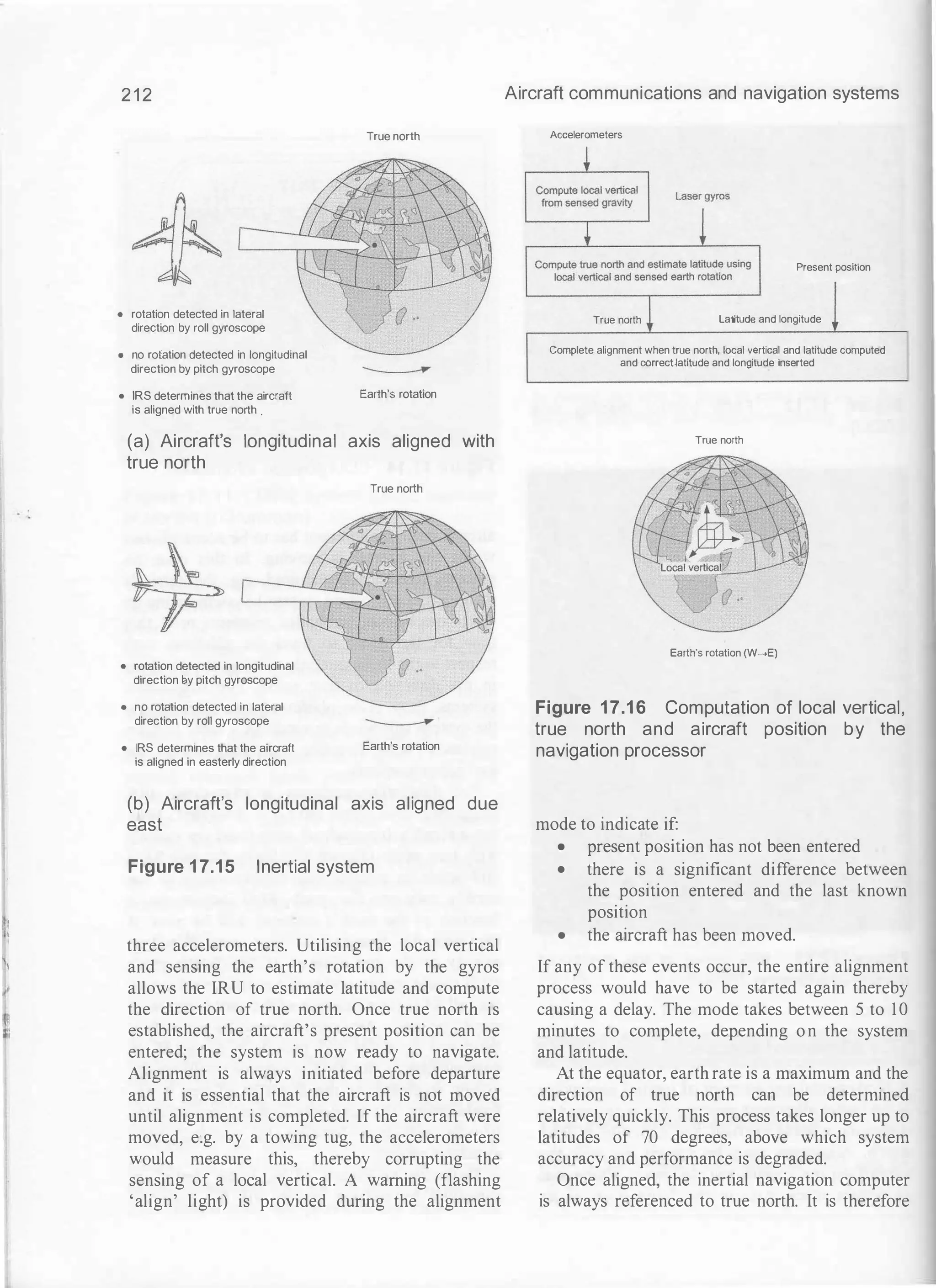
![1 96 Aircraft communications and navigation systems ·
Above 3000'
•
I
I
:=====]----.�
A
irfield
I
I
I
I
:
------IL�=======I----l---+�... At6000'
: ----
-
-
-
- - - - /
1
I
I
I
: __ .,. - -
-
_/8-"
VOR-DME(1)
•
.,,..;"'
...
�
--
-
-
-
-
-
-
-
-
-
�
,-
-
-
-
-
-
-
--+ 8�>
Above 3000' At 6000'
VOR-DME (2)
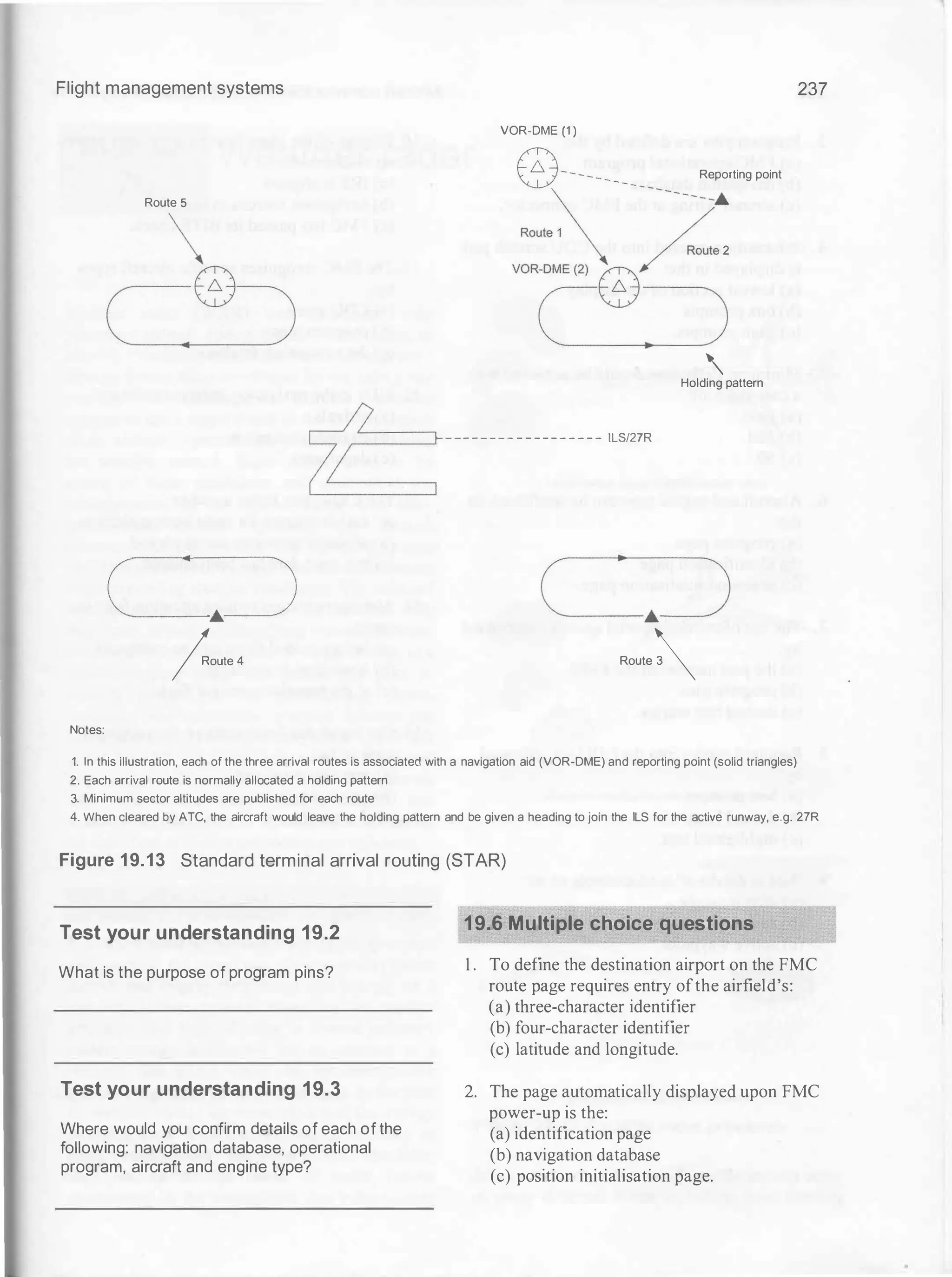
Notes:
1 . In this illustration, each of the three runways has a specific departure route to the VOR-DME (2) navigation aid; the aircraft then joins the airways network
2. The SIDs are typically referenced to navigation aids. e.g. VOR-DME or marker beacons
3. There would also be published departure routes for aircraft joining airways to the south, east and north
4. Reporting points (triangles) are often specified with altitude constraints, e.g. at. below or above 3000'
Figure 1 6.13 Illustration of standard instrument departures (SID)
Test your understanding 16.1
Give (a) three features and (b) three benefits of
RNAV.
Test your understanding 16.2
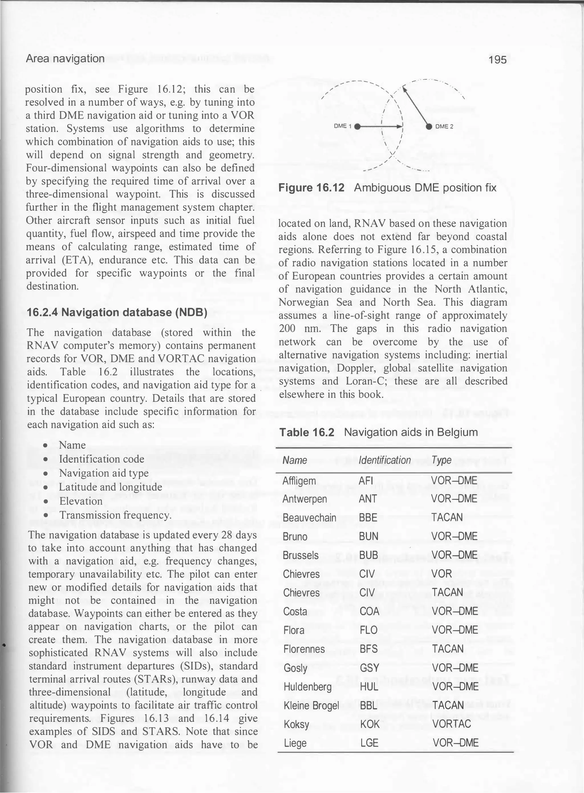
The navigation database contains permanent
records for radio navigation aids. List the typical
information that is stored for each one.
Test your understanding 16.3
What feature is used to select the best navigation
aids for optimised area navigation?
16.3 Kalman filters
One essential feature ofadvanced RNAV systems
is the use of Kalman filters, named after Dr
Richard Kalman who introduced this concept in
the 1 960s. Kalman filters are optimal recursive
data processing algorithms that filter navigation
sensor measurements. The mathematical model is
based on equations solved by the navigation
processor. To illustrate the principles of Kalman
filters, consider an RNAV system based on
inertial navigation sensors with periodic updates
from radio navigation aids. (Inertial navigation is
described in Chapter 1 7.) One key operational
aspect of inertial navigation is that system errors
accumulate with time. When the system receives
a position fix from navigation aids, the inertial
navigation system's errors can be corrected.
The key feature of the Kalman filter is that it
can analyse these errors and determine how they
might have occurred; the filters are recursive, i.e.
they repeat the correction process on a succession
of navigation calculations and can 'learn' about](https://image.slidesharecdn.com/aircraftcommunicationsandnavigationsystemsprinciplesoperationandmaintenancepdfdrive-250205173033-c029e156/75/Aircraft-communications-and-navigation-systems_-principles-operation-and-maintenance-PDFDrive-pdf-206-2048.jpg)
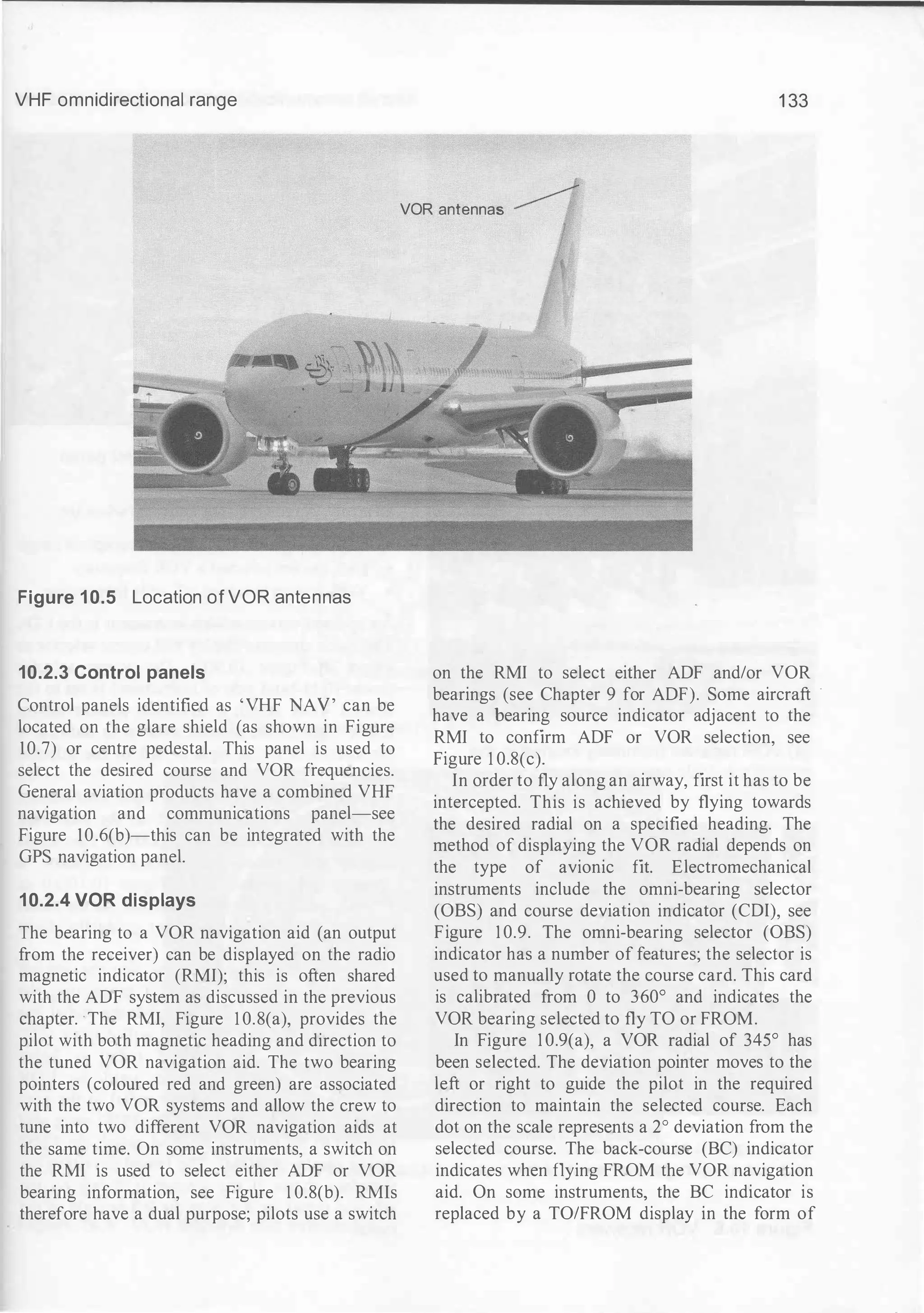
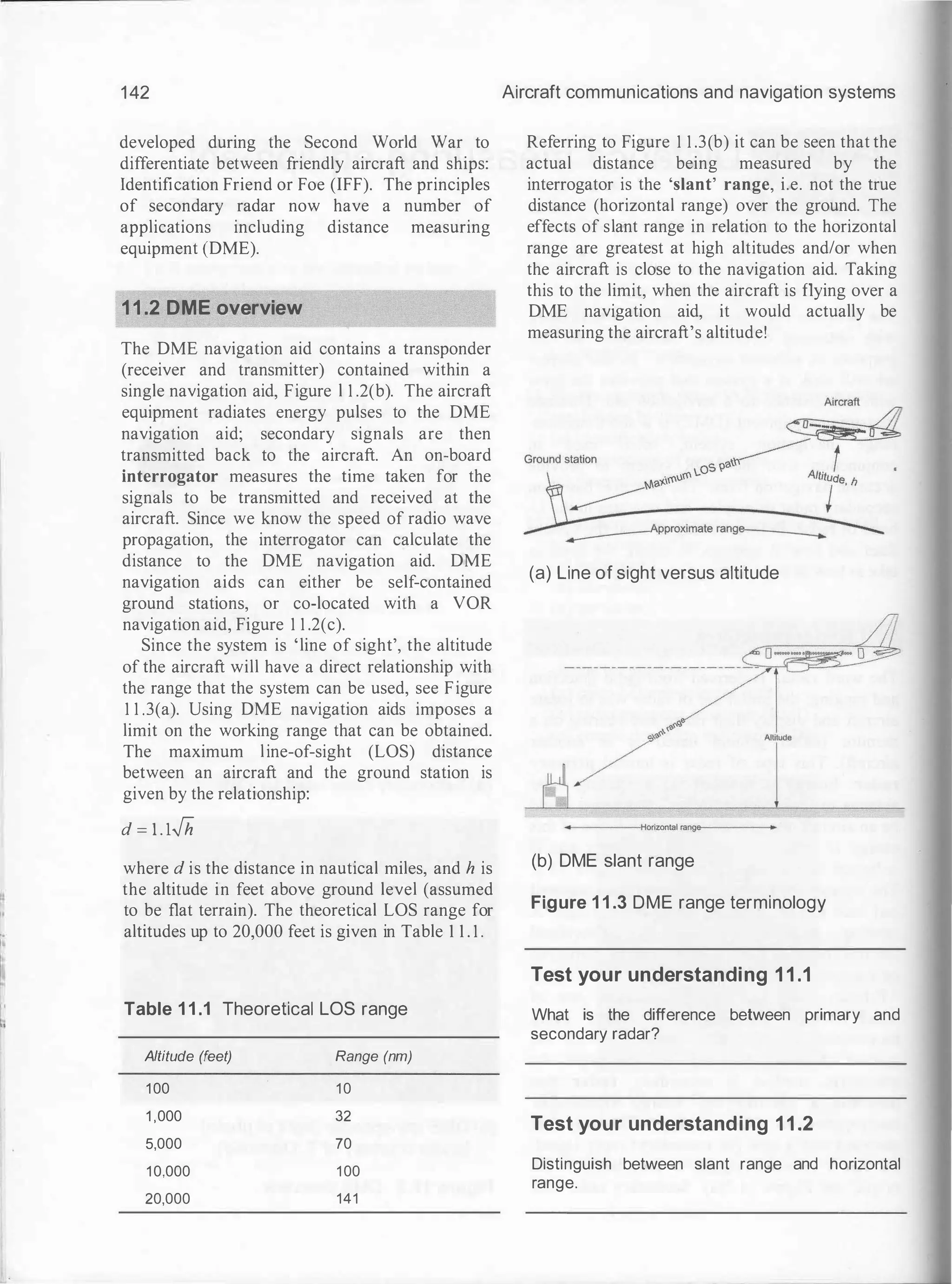
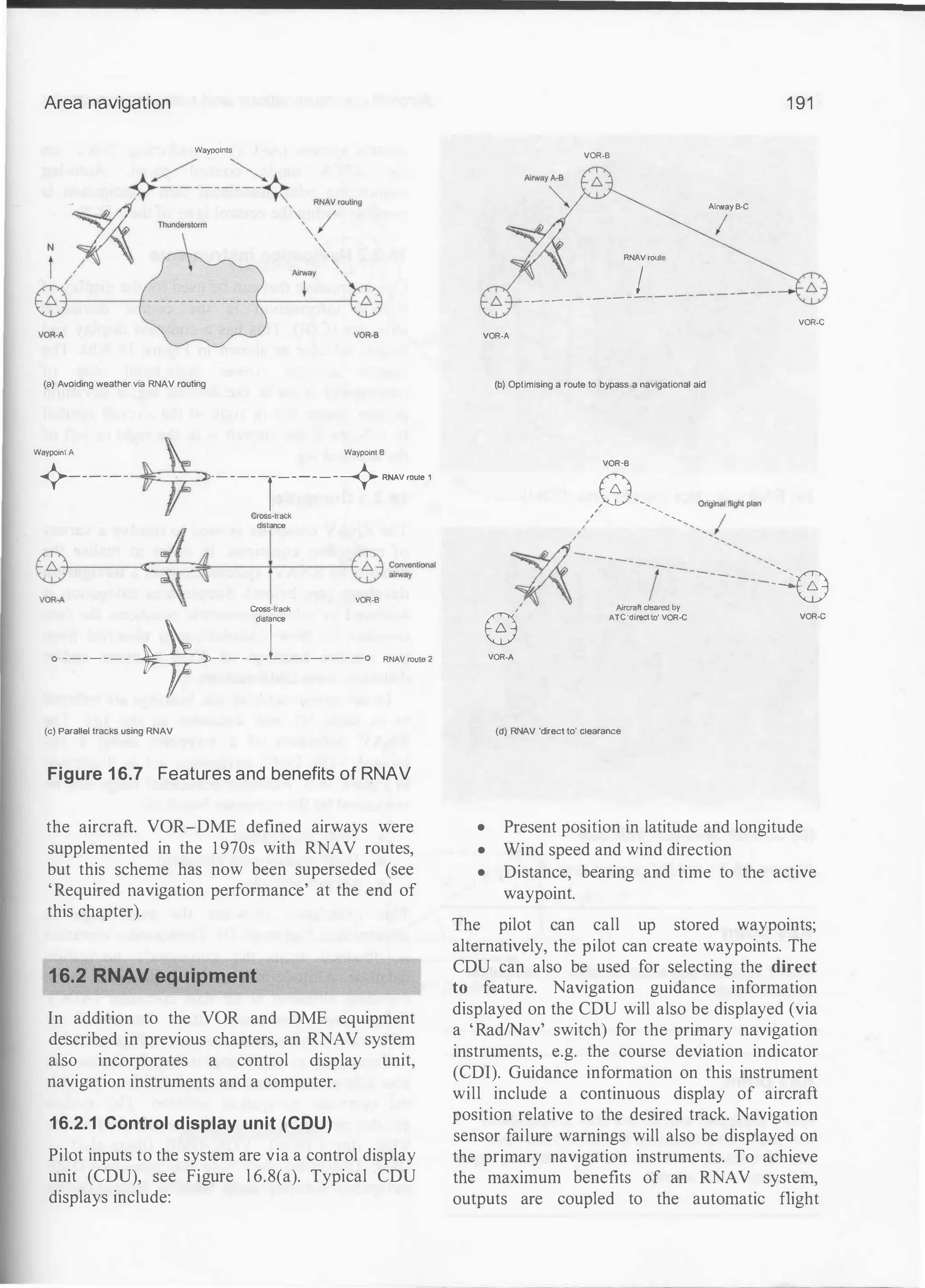
![Inertial navigation system
r - - - -
Control display unit (CDU)
f--i---i� Attitude displays
j N Y l i 5 6 jw : 2 : 2 Y I I
Inertial references
(accelerometers and gyros)
f--r--i� Autopilot references
CJ ITJ [J
[I] OJ
CJ [JJ [J
B eJ El 'l
Navigation processor
!+--+-- Air data computer
(true airspeed)
Mode select unit (MSU)
NAV
Memory
I
I
I
I
I
I
Inertial navigation unit (INU) :
_ _ _ _ _ _ _ _ _ _ _ _ _ _ _ _ _ _ _ _ _ J
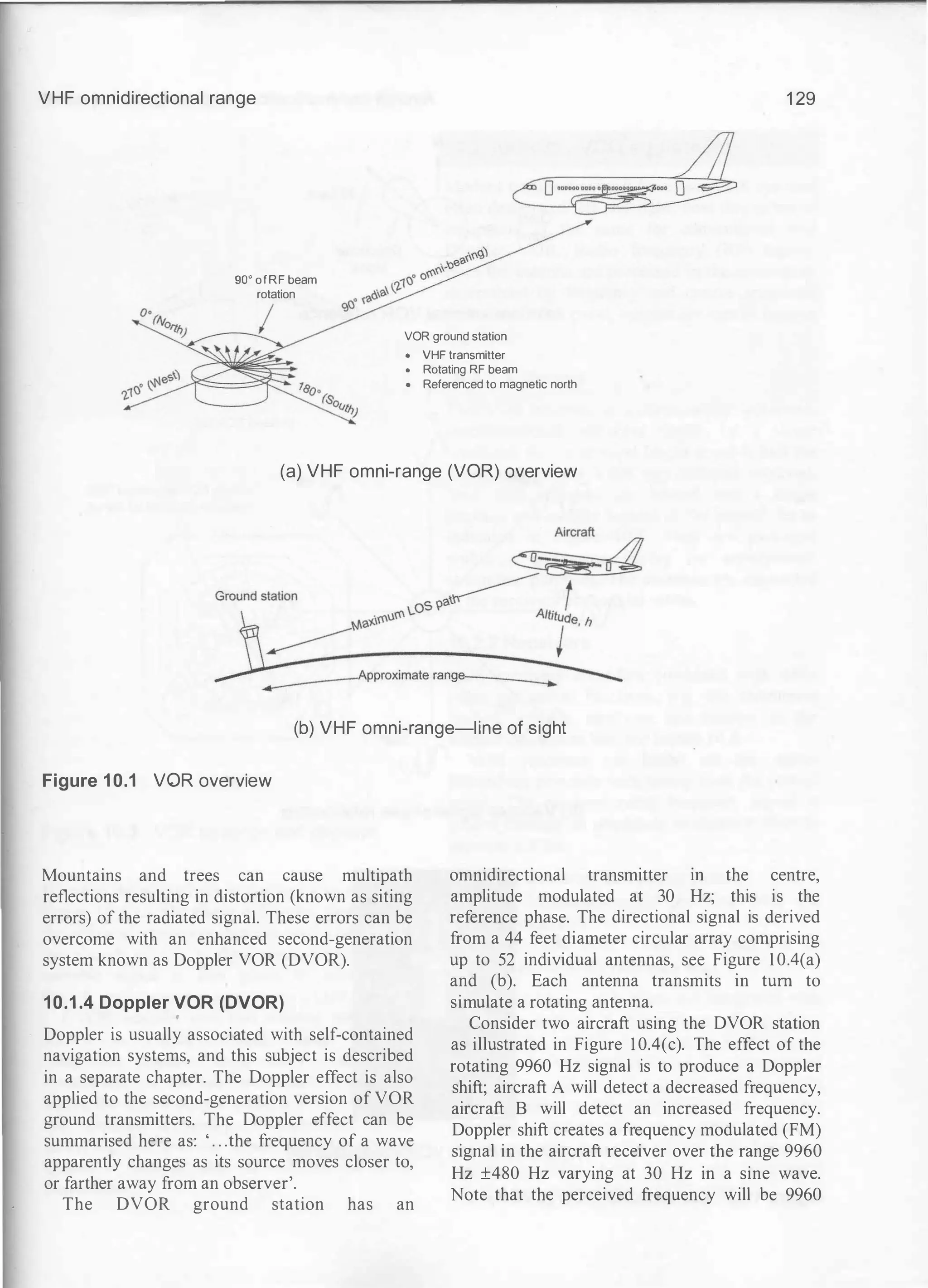
Figure 1 7.6(a) Inertial navigation system (general arrangement)
Figure 1 7.6(b) Inertial navigation system (courtesy of Northrop Grumman)
Key point Key point
Battery
205
Synthesised magnetic variation can be obtained
from inertial navigation systems meaning that
remote sensing compass systems are not
required.
By comparing the position outputs of three on
board inertial navigation systems, this also
provides a means of error checking between
systems.](https://image.slidesharecdn.com/aircraftcommunicationsandnavigationsystemsprinciplesoperationandmaintenancepdfdrive-250205173033-c029e156/75/Aircraft-communications-and-navigation-systems_-principles-operation-and-maintenance-PDFDrive-pdf-215-2048.jpg)
![Flight management systems
Ambient light sensor Five inch CRT with
1 4 lines x 24 character lines
Line select keys
§] IT[] � lvNAvl
Function and
mode keys
ILEGsl IHOLDI lto",C"I IPRoGI
Annunciators -
'-----v---" '----�---'
Numeric keys Alphabetic keys
Figure 19.2 Location of FMCS control and display unit
aircraft is shown in Figure 19. 1 . The CDU
comprises a variety of features, referring to
Figure 1 9.2 these include the:
• data display area (typically a cathode ray
tube-CRT)
• line-select keys (LSK)
• function and mode keys
• alpha-numeric key pad
• warning annunciators.
The display area is arranged in the form of
chapters and pages of a book. When the system is
first powered up, the CDU displays the IDENT
page, see Figure 1 9.3.
Line select keys
CRT brightness
adjustment
- Annunciators
229
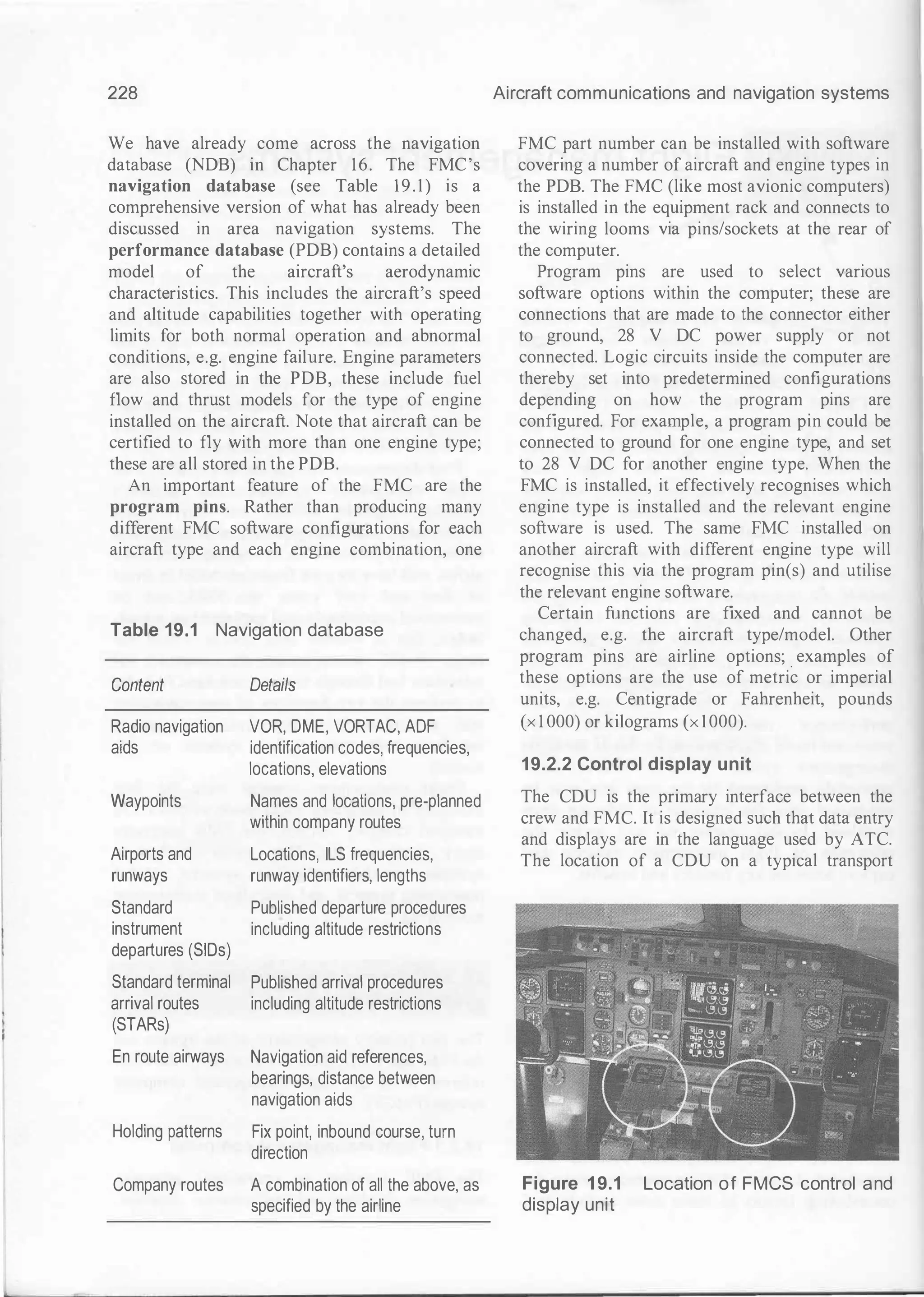
The 'IDENT' page contains basic information
as stored in the FMC including aircraft model,
engine types etc. Other pages are accessed from
this page on a menu basis using the line-select
keys, or directly from one ofthe function or mode
select keys.
Figure 19.3 'IDENT' page displayed on
system power-up](https://image.slidesharecdn.com/aircraftcommunicationsandnavigationsystemsprinciplesoperationandmaintenancepdfdrive-250205173033-c029e156/75/Aircraft-communications-and-navigation-systems_-principles-operation-and-maintenance-PDFDrive-pdf-239-2048.jpg)
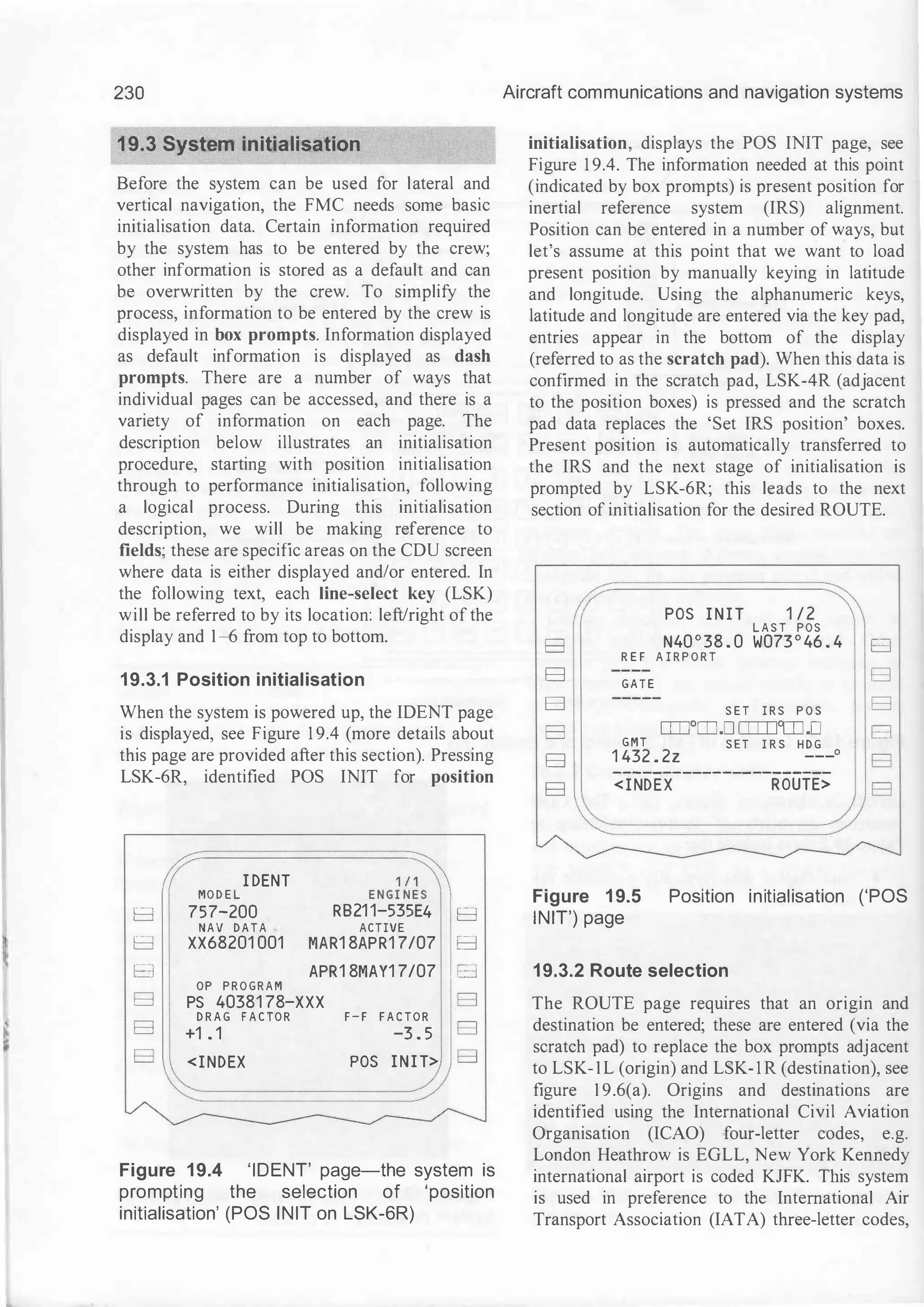
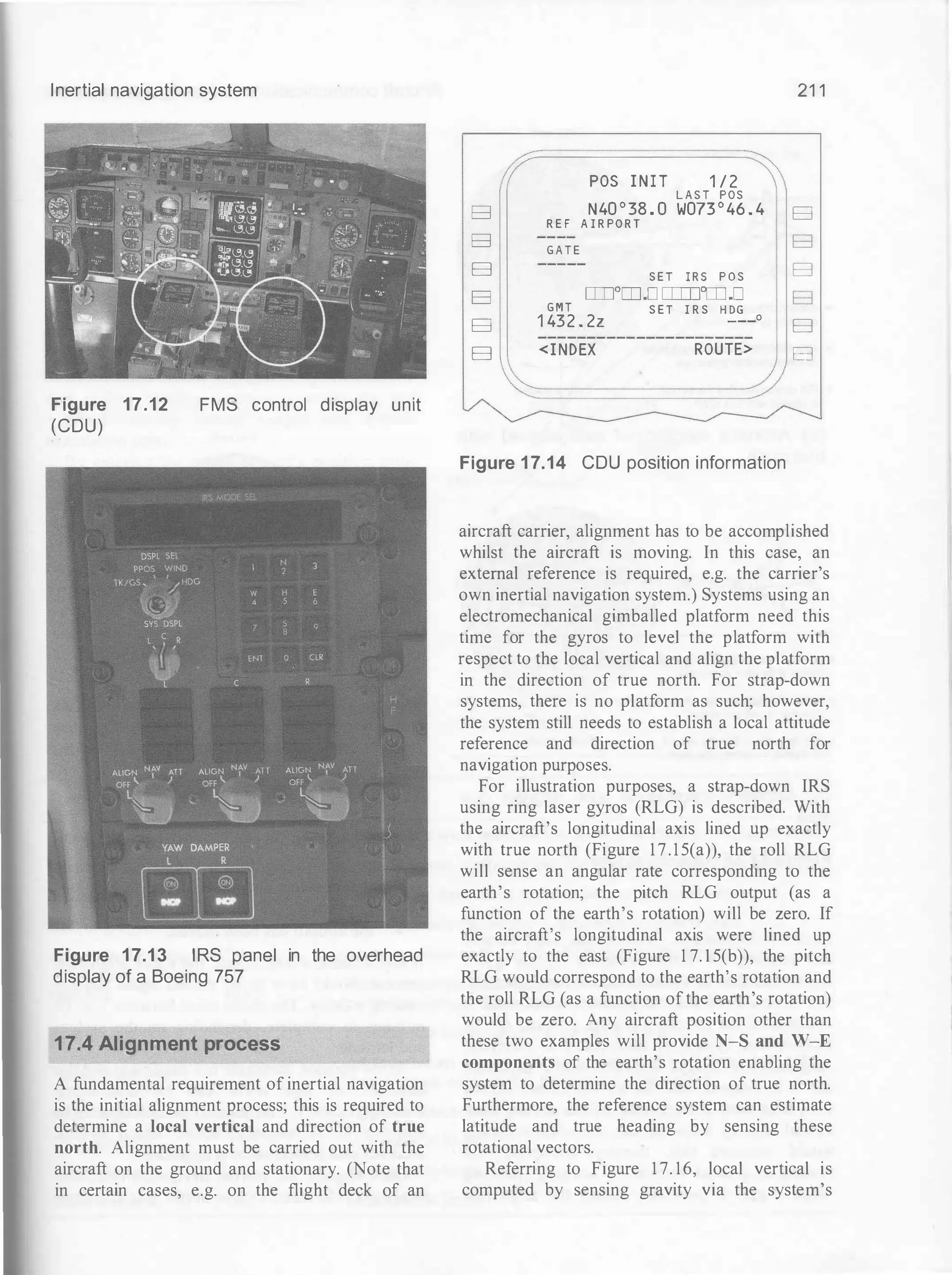
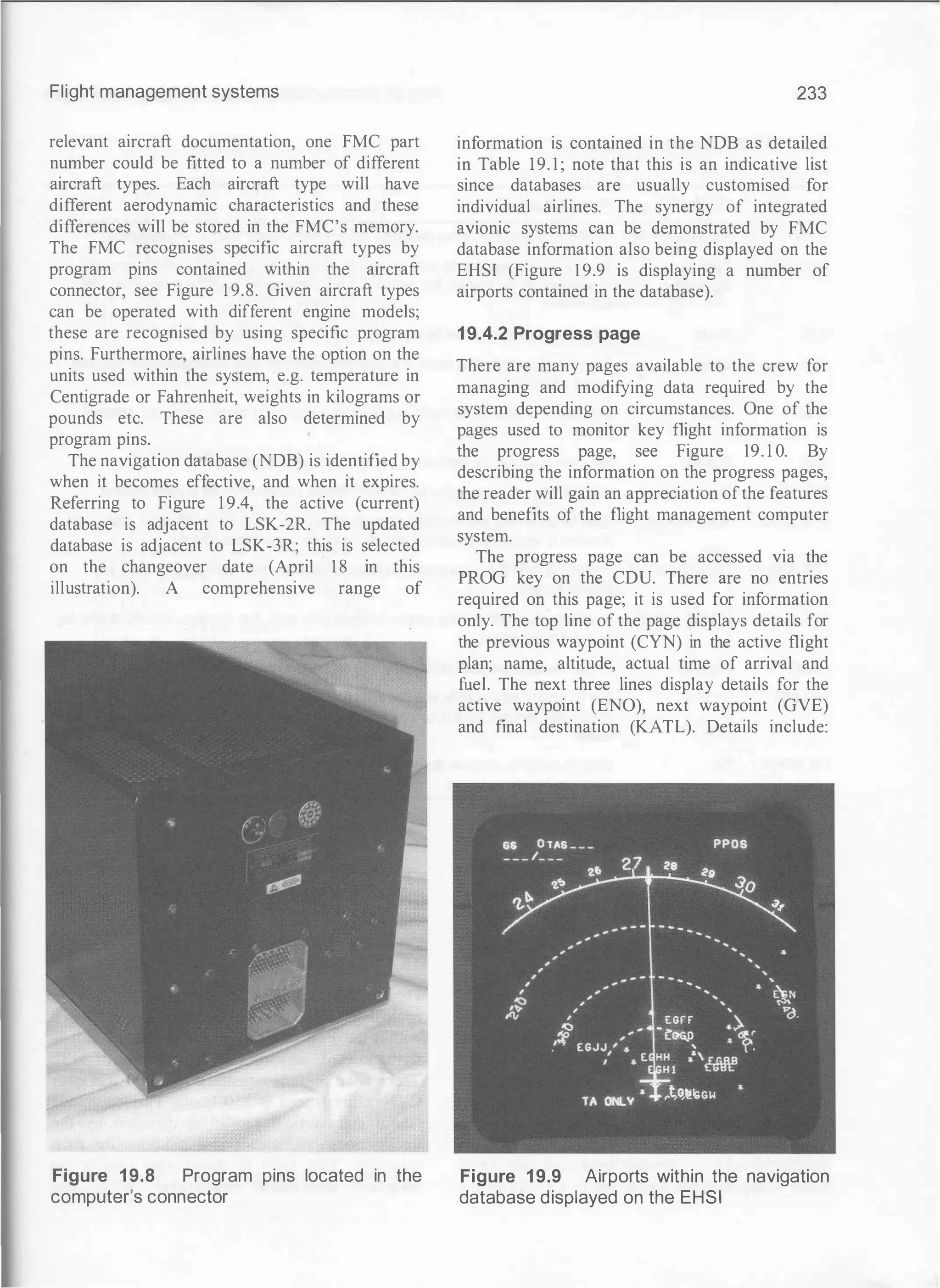
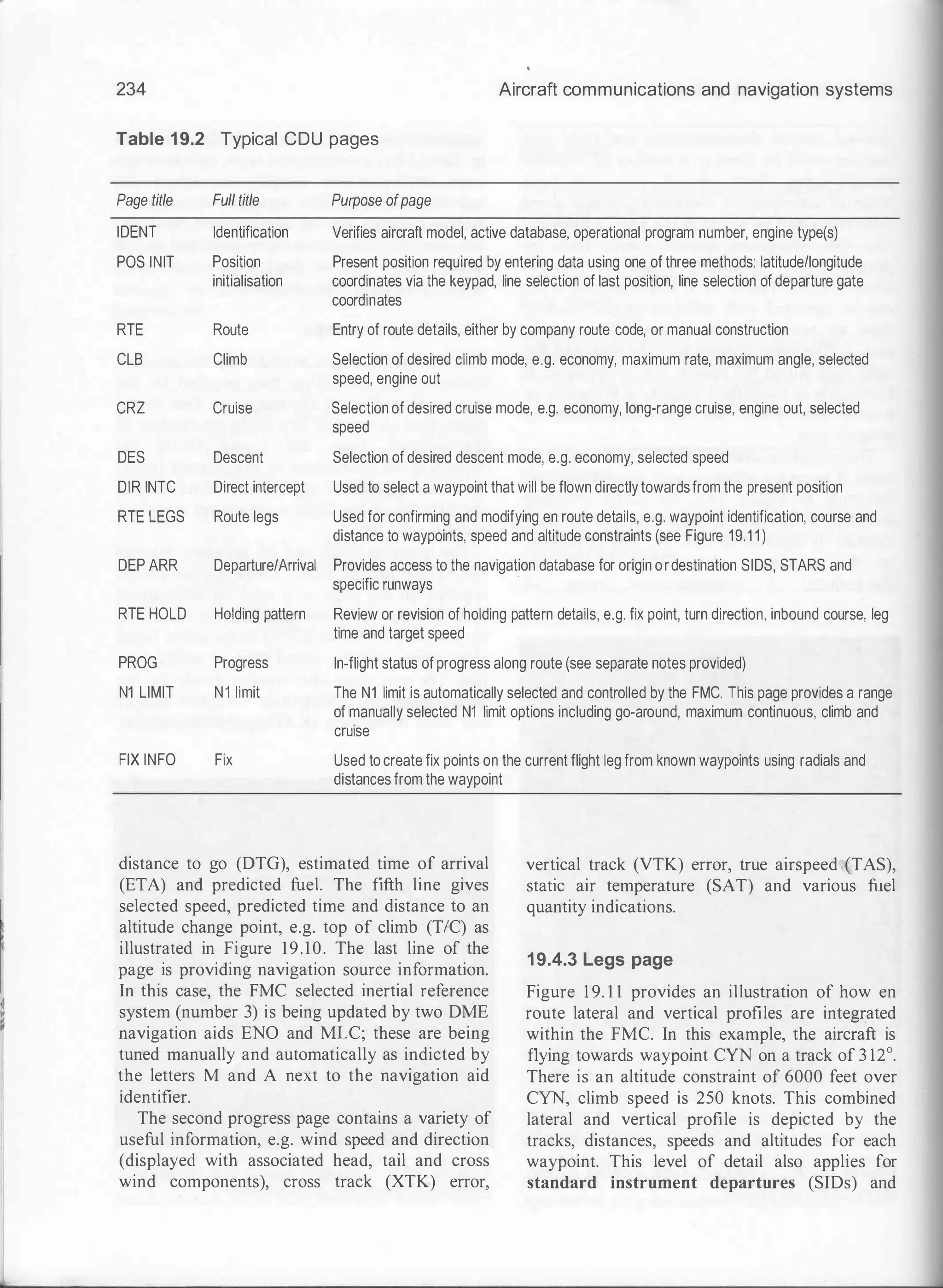
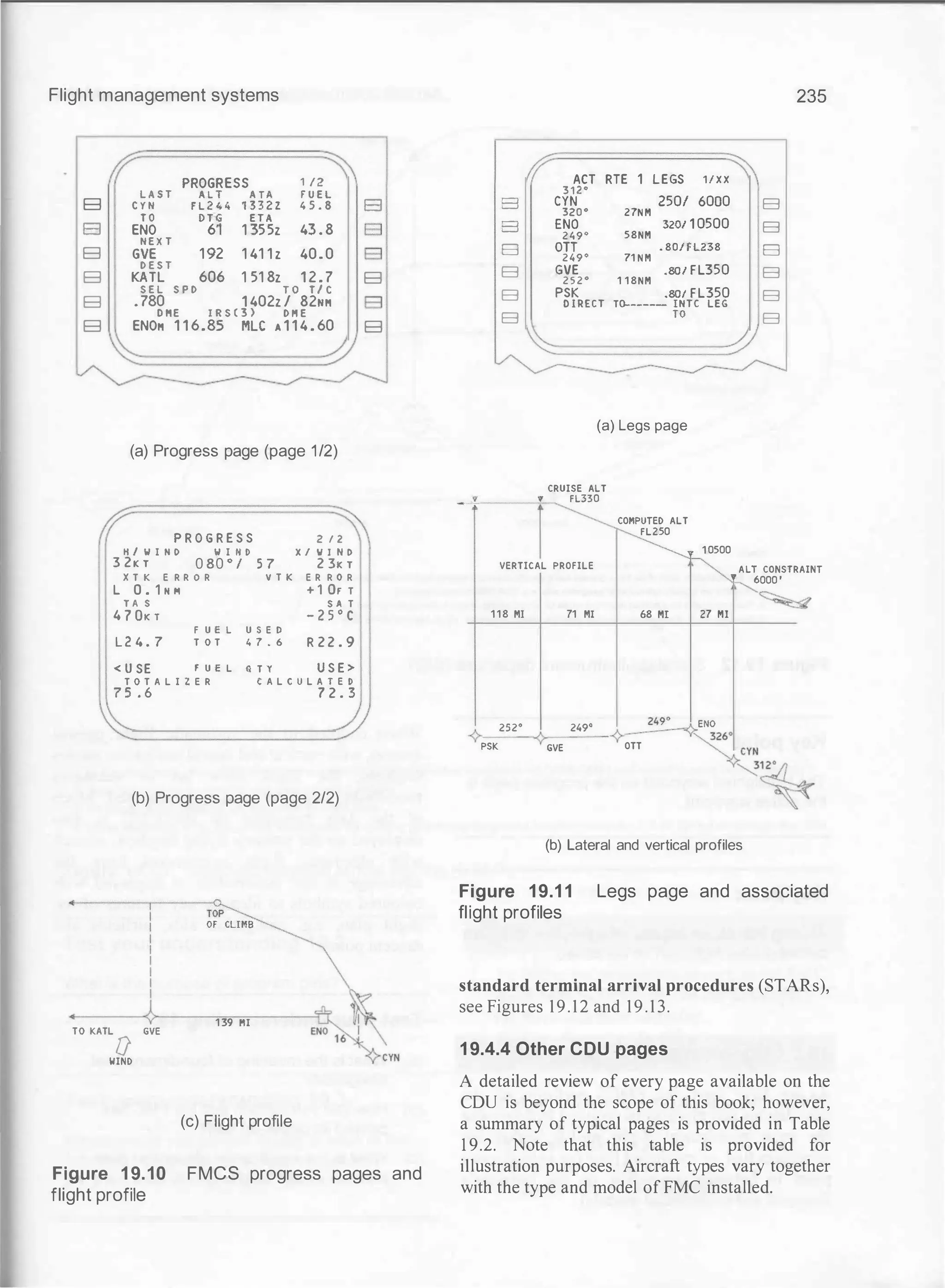
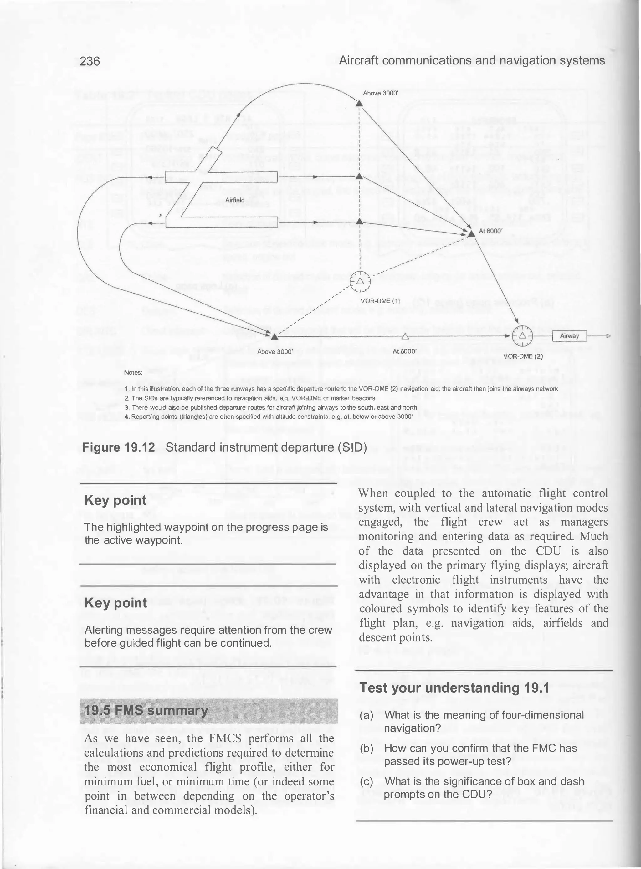
![232
contained within the company route. All other
entries on the page are optional; entry of data in
these fields will enhance system performance.
Once the performance initialisation details are
confirmed, the system is ready for operation.
Further refinement of the flight profile can be
made by entering other details, e.g. take-off
settings, standard instrument departures, wind
forecasts etc.
B
B
B
B
B
B
PERF
G R O S S W T
DJJ .D
F U E L
52 . 3
Z F W
DJJ.D
R E S E R V E S
rn .o
C O S T I N D E X
ITO
< I NDEX
I N I T 1 / 1
C R Z A L T
[[[]]]
C R Z W I N D
___ o /---
I S A D E V
___ o c
T I C O A T
___
o c
T R A N S A L T
1 8000
TAKEO F F>
B
B
B
B
B
B
Figure 1 9.7 Performance initialisation
('PERF INIT') page
19.4 FMCS operation
The flight management computer system
(FMCS) calculates key performance data and
makes predictions for optimum operation of the
aircraft based on the cost-index. We have already
reviewed the system initialisation process, and
this will have given the reader an appreciation of
how data is entered and displayed. The detailed
operation of a flight management system is
beyond the scope of this book; however, the key
features and benefits of the system will be
reviewed via some typical CDU pages. Note that
these are described in general terms; aircraft
types vary and updated systems are introduced on
a periodic basis. CDU pages can be accessed at
any time as required by the crew; some pages can
be accessed via the line-select keys as described
in section 19.3; some pages are accessed via
function/mode keys. The observant reader may
Aircraft communications and navigation systems
Key point
The FMS comprises the following subsystems:
FMCS, AFCS and IRS.
Key point
The page automatically displayed upon FMC
power-up is the identification page; this confirms
that the FMC has passed a sequence of self-tests.
Key point
Required entries into the CDU are indicated by
box prompts; optional entries are indicated by
dashed line prompts.
Key point
To define the destination airport on the FMC route
page requires entry of the airfield's four-character
identifier.
have already noticed that in the top right of each
CDU page is an indication of how many sub
pages are available per selected function.
19.4.1 Identification page ('IDENT')
This page is automatically displayed upon power
up; aside from displaying a familiar page each
time the system is used, this also serves as
confirmation that the FMC has passed a sequence
of built-in test equipment (BITE) self-tests
including: memory device checks, interface
checks, program pin configuration, power
supplies, software configurations and
microprocessor operation. Information displayed
on this page includes aircraft and engine types,
navigation database references and the
operational program number. By reference to the](https://image.slidesharecdn.com/aircraftcommunicationsandnavigationsystemsprinciplesoperationandmaintenancepdfdrive-250205173033-c029e156/75/Aircraft-communications-and-navigation-systems_-principles-operation-and-maintenance-PDFDrive-pdf-242-2048.jpg)


![A presentation on internship from jaipur Airport [AAI]](https://cdn.slidesharecdn.com/ss_thumbnails/airportpptbyadityasept-160404162154-thumbnail.jpg?width=640&height=640&fit=bounds)


