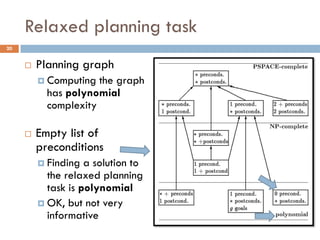
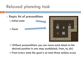
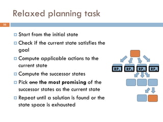
Download as PDF, PPTX


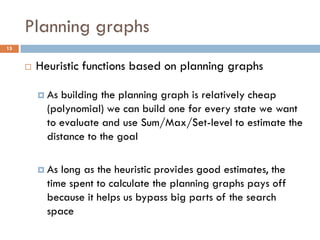

![Relaxed planning task: hadd, hmax
26
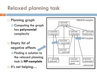
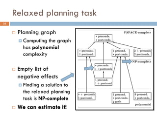
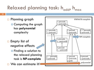
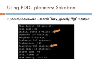
Build a graph that approximates the cost of achieving
literal p from state s [Bonet, Geffner 2001]
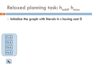
Initializethe graph with literals in s having cost 0
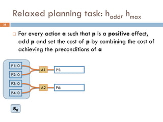
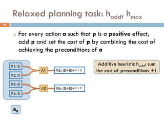
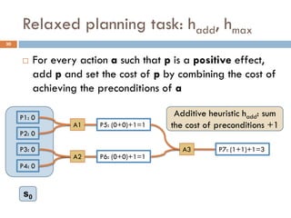
For every action a such that p is a positive effect, add p
and set the cost of p by combining the cost of achieving
the preconditions of a
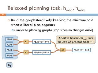
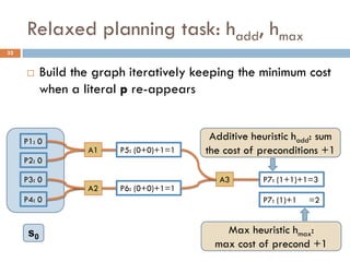
Build the graph iteratively keeping the minimum cost when
a literal p re-appears
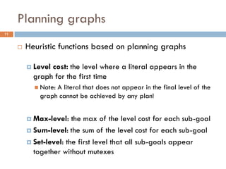
The way the cost is combined for two literals defines the
heuristic: hadd, hmax](https://image.slidesharecdn.com/aigames-lecture4-part2-121022052221-phpapp02/85/Intro-to-AI-STRIPS-Planning-Applications-in-Video-games-Lecture4-Part2-26-320.jpg)
![Relaxed planning task: hadd, hmax
38
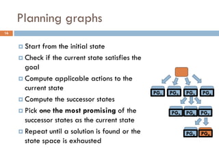
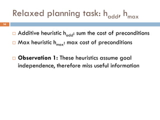
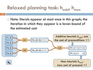
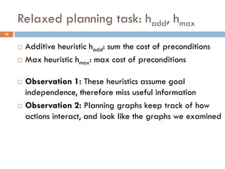
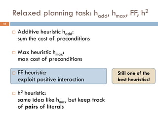
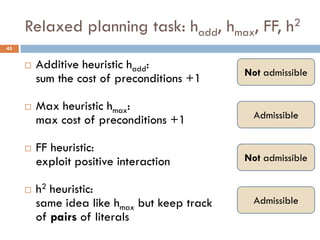
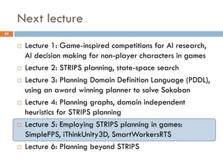
Additive heuristic hadd: sum the cost of preconditions
Max heuristic hmax: max cost of preconditions
Observation 1: These heuristics assume goal
independence, therefore miss useful information
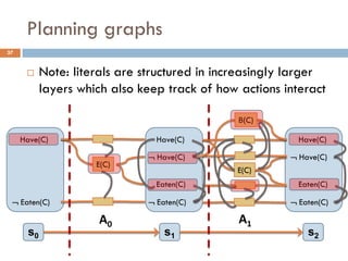
Observation 2: Planning graphs keep track of how
actions interact, and look like the graphs we examined
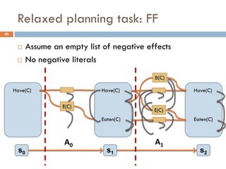
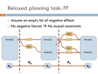
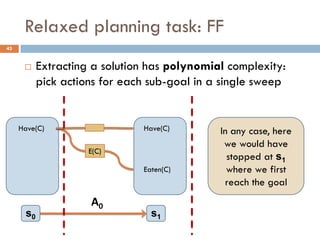
FF Heuristic: Let’s apply the empty delete list
relaxation to planning graphs!
[Hoffmann, Nebel 2001]](https://image.slidesharecdn.com/aigames-lecture4-part2-121022052221-phpapp02/85/Intro-to-AI-STRIPS-Planning-Applications-in-Video-games-Lecture4-Part2-38-320.jpg)


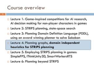
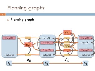
The document outlines a course by Stavros Vassos on AI and its applications in video games, focusing on various planning techniques like STRIPS and planning graphs. It discusses the complexity and methodologies of planning algorithms, including heuristic functions and relaxed planning tasks, emphasizing their benefits in decision-making for non-player characters in games. The lectures aim to provide a comprehensive understanding of AI decision-making structures and their practical implementations in game design.