
![Eg: job scheduling, variables are start/end days for each job
• Need a constraint language
Eg: StartJob1 +5 ≤ StartJob3.
• Linear constraints solvable, nonlinear undecidable.
ii. Continuous variables
• Linear constraints solvable in poly time by linear programming methods
(deal with in the field of operations research).
iii. Our focus: discrete variables and finite domains
iv. Unary constraints involve a single variable.
E.g. SA ≠ green
v. Binary constraints involve pairs of variables.
E.g. SA ≠ WA
vi. Global constraints involve an arbitrary number of variables.
Eg: Crypth-arithmetic column constraints.
• Preference (soft constraints) e.g. red is better than green often represent able
by a cost for each variable assignment; not considered here.
REAL WORLD CSP’s:
• Assignment problems
• E.g., who teaches what class
• Timetable problems
• E.g., which class is offered when and where?
• Transportation scheduling
• Factory scheduling
CSP as a standard search problem:
Incremental formulation:
• States: Variables and values assigned so far
• Initial state: The empty assignment
• Action: Choose any unassigned variable and assign to it a value that does not
violate any constraints
• Fail if no legal assignments
• Goal test: The current assignment is complete and satisfies all constraints.
• Same formulation for all CSPs!!!
• Solution is found at depth n (n variables).
• What search method would you choose?
• How can we reduce the branching factor?
Commutative:
• CSPs are commutative.
• The order of any given set of actions has no effect on the outcome.
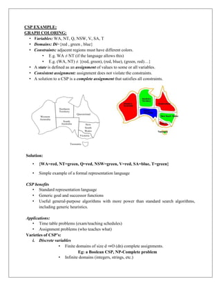
• Example: choose colors for Australian territories one at a time
• [WA=red then NT=green] same as [NT=green then WA=red]
• All CSP search algorithms consider a single variable assignment at a time
⇒ there are dn leaves.](https://image.slidesharecdn.com/unitiiinotesmerged-240124060841-16af7ff8/85/AI3391-Artificial-Intelligence-UNIT-III-Notes_merged-pdf-23-320.jpg)

![8. CONSTRATIN PROPAGATION:
In local state-spaces, the choice is only one, i.e., to search for a solution. But in CSP, we have
two choices either:
We can search for a solution or
We can perform a special type of inference called constraint propagation.
Constraint propagation is a special type of inference which helps in reducing the legal
number of values for the variables.
The idea behind constraint propagation is local consistency.
In local consistency, variables are treated as nodes, and each binary constraint is treated as
an arc in the given problem.
There are following local consistencies which are discussed below:
1. Node Consistency: A single variable is said to be node consistent if all the values in the
variable’s domain satisfy the unary constraints on the variables.
2. Arc Consistency: A variable is arc consistent if every value in its domain satisfies the binary
constraints of the variables.
3. Path Consistency: When the evaluation of a set of two variables with respect to a third
variable can be extended over another variable, satisfying all the binary constraints. It is similar
to arc consistency.
4. k-consistency: This type of consistency is used to define the notion of stronger forms of
propagation. Here, we examine the k-consistency of the variables.
9. BACKTRACKING CSP’s:
• In CSP’s, variable assignments are commutative
For example:
[WA = red then NT = green]
Is the same as?
[NT =green then WA = red]](https://image.slidesharecdn.com/unitiiinotesmerged-240124060841-16af7ff8/85/AI3391-Artificial-Intelligence-UNIT-III-Notes_merged-pdf-27-320.jpg)

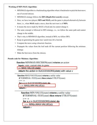
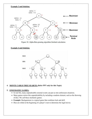
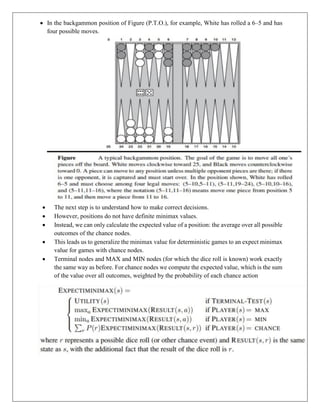
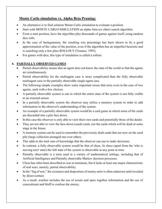
The document provides information about game playing and constraint satisfaction problems (CSP). It discusses adversarial search techniques like minimax algorithm and alpha-beta pruning that are used for game playing. The minimax algorithm uses recursion to search through the game tree and find the optimal move. Alpha-beta pruning improves on minimax by pruning parts of the tree that are guaranteed not to affect the outcome. The document also mentions other topics like Monte Carlo tree search, stochastic games with elements of chance, and formalization of game state, actions, results, and utilities.