This document compares the aerodynamic characteristics of the NACA 0012 airfoil from wind tunnel and XFOIL calculations at an angle of attack of 60 degrees. Wind tunnel pressure measurements were taken at 23 points on the airfoil surface. XFOIL was run to calculate pressure coefficients for comparison. The results show good agreement between the two methods, with less than 17.1% error in lift coefficient.

1. Islam Mansour | OA1-A Aerodynamics I | November 12, 2015
Report I
AERODYNAMIC CHARACTERISTICS FOR AIRFOIL NACA 0012 @ +60
SUBMITTED TO: ING. ROBERT POPELA, PH.D.
ING. ONDŘEJ LAJZA

2. PAGE 1
Contents
Exercise I the NACA 0012 airfoil comparison between characteristic from Wind Tunnel and XFOIL
at 60
angles of attack..................................................................................................................................2
Wind Tunnel measurement and Calculation.....................................................................................2
The data taken from the wind tunnel was at the angle of attack equal +6 degree ...........................3
Xfoil Calculation.................................................................................................................................4
Conclusion ..........................................................................................................................................5
Appendix ....................................................................................................................................................6
Matlab code.........................................................................................................................................7
Xfoil Command................................................................................................................................. 10
Figure 1: Airfoil NACA 0012 .......................................................................................................................2
Figure 2: schematic for the wind tunnel measurement...........................................................................2
Figure 3: measured coefficient of pressure Cp..........................................................................................4
Figure 4: Xfoil calculated coefficient of pressure Cp ...............................................................................4
Figure 5: Pressure vector around the airfoil.............................................................................................5
Figure 6: plot for xfoil and wind tunnel Cp...............................................................................................5

3. PAGE 2
Figure 2: schematic for the wind tunnel measurement
Exercise I the NACA 0012 airfoil comparison between
characteristic from Wind Tunnel and XFOIL at 60
angles of attack
The Airfoil NACA 0012 is a symmetric airfoil which is a part of the NACA four-digit series.
That the first digit representing maximum camber as a percent of the cord “C”; the second digit
representing the location of the maximum chamber from the leading edge as a percent of the cord –
“C”; the last two digit representing the maximum chamber thickness as a percent of the chord “C”.
Wind Tunnel measurement and Calculation
The wind tunnel uses a pressure transducer which measure the difference of the pressure.
There is a twenty-three (23) pressure transducer twelve (12) of it along the upper surface of the airfoil
and eleven (11) on the lower surface of the airfoil. In addition, three pressure transducer, two of it at
the entrance of the wind tunnel to measure atmosphere pressure and static pressure. So total drag
coefficient drag would be calculated from the equation, where CDo represents the pressure drag.
𝐶 𝐷 = 𝐶 𝐷𝑜 + 𝐶𝑓
Figure 1: Airfoil NACA 0012

4. PAGE 3
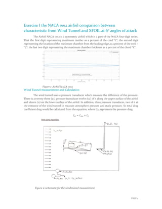
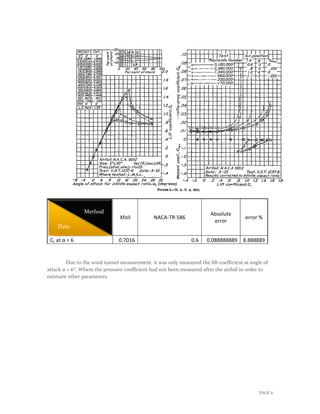
The data taken from the wind tunnel was at the angle of attack equal +6 degree
The atmospheric pressure measured at the entrance of the wind tunnel and is called in
data Bar_pressure which is needed to multiply by 100 to convert it Pa where Patm = 98320.3822 Pa,
Dynamic pressure = 555.0319857 Pa, and P∞ = 97765 Pa.
Lower airfoil surface
sequence from LE pressure reading # position x/c [-] Cp
1 -131.903 0.0053 0.7623501
2 -305.584 0.0272 0.4494307
3 -545.518 0.0724 0.0171415
4 -547.228 0.1235 0.0140613
5 -584.756 0.1985 -0.053553
6 -612.031 0.2981 -0.102695
7 -618.363 0.3977 -0.114103
8 -627.104 0.4973 -0.129852
9 -620.01 0.5963 -0.117071
10 -612.916 0.6959 -0.10429
11 -606.2 0.7955 -0.09219
12 -599.484 0.8984 -0.080089
Upper airfoil surface
sequence from LE pressure reading # position x/c [-] Cp
1 -1513.414 0.0133 -1.726716
2 -1289.263 0.0511 -1.322862
3 -1255.726 0.1023 -1.262439
4 -1083.976 0.1547 -0.952998
5 -890.8852 0.2543 -0.605106
6 -819.067 0.3559 -0.475711
7 -812.4952 0.4542 -0.463871
8 -768.86 0.5518 -0.385254
9 -725.2249 0.6527 -0.306636
10 -693.7345 0.755 -0.2499
11 -631.7935 0.8586 -0.138301

5. PAGE 4
The measured lift coefficient from wind tunnel is equal to CL = 0.5820
Xfoil Calculation
Xfoil was performed the same calculation for NACA 0012 airfoil in order to make
compression between wind tunnel measurement and verifying it. Here it is the results:
Figure 4: Xfoil calculated coefficient of pressure Cp
Figure 3: measured coefficient of pressure Cp

6. PAGE 5
Figure 5: Pressure vector around the airfoil
Conclusion
It is concluded that difference between wind tunnel measurements for NACA 0012 air foil
for low angle of attack is almost near to Xfoil theoretical calculation. Where CL = 0.5820 according
to wind tunnel and CL= 0.7016 according to Xfoil with error less than 17.1 %. However, three pressure
transducers weren’t working so it was necessary to make linear approximations for this missing
values. As show in the figure 6, that is a compression between Cp from the wind tunnel and Xfoil.
Figure 6: plot for xfoil and wind tunnel Cp

7. PAGE 6
Xfoil NACA-TR-586
Absolute
error
error %
CL at α = 6 0.7016 0.6 0.088888889 8.888889
Due to the wind tunnel measurement, it was only measured the lift coefficient at angle of
attack α = 60
. Where the pressure coefficient had not been measured after the airfoil in order to
estimate other parameters.
Data
Method

8. PAGE 7
Appendix
Matlab code
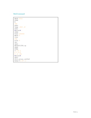
%% *This code for wind tunnel measurement to calculate the lift of NACA
0012 @ +6 deg*
clc;
clear all;
close all;
%%
load('airfoil_0012_6.mat')
P_atm = 983.203822*100; % multi * 100 due to hPa to Pa
% A = importdata(n0012.txt)
Dyn_pressure = 555.0319857; %Dynamic pressure where is it "q_inf" P_1
P_inf = P_atm - Dyn_pressure; % Pressure_1 at the entrace of windtunel
% P_2 = 522.8432576; % pressure after the airfoil
P_up = [-131.9032846
-305.5835476
-545.5179151
-547.2275195
-584.7557098
-612.0307604
-618.363024
-627.103931
-620.0101133
-612.9162957
-606.2001103
-599.483925];
P_up = P_atm + P_up;
%P_up = -P_up;
%pressure at the upper surface
P_lo = [-1513.414499
-1289.2627
-1255.726162
-1083.976227
-890.8851534
-819.0669726
-812.4951664
-768.8600403
-725.2249142
-693.7344964
-631.793477];
P_lo = P_atm + P_lo;
%P_lo = norm(p_lo,2);
% pressure at the lower surface from P_17 to P_27
xc_up = [0.0053
0.0272

9. PAGE 8
0.0724
0.1235
0.1985
0.2981
0.3977
0.4973
0.5963
0.6959
0.7955
0.8984];
%cord ratio for upper surface sensor
xc_lo = [0.0133
0.0511
0.1023
0.1547
0.2543
0.3559
0.4542
0.5518
0.6527
0.755
0.8586];
%cord ratio for lower surface sensor
yc_up = [0.012553011
0.027129251
0.041375966
0.050335162
0.05727481
0.060006371
0.058099622
0.053094655
0.045924736
0.037031823
0.026722114
0.014672403];
%camber for upper suface
yc_lo = [0.019420256
0.035818939
0.047166286
0.053887512
0.059501721
0.059335197
0.055572188
0.049379552
0.041078327
0.031073771
0.019509279];
%camber for lower suface
cp_up = (P_up - P_inf) / Dyn_pressure;
cp_lo = (P_lo - P_inf) / Dyn_pressure;

10. PAGE 9
Cn_up = trapz(xc_up, cp_up)
Cn_lo = trapz(xc_lo, cp_lo)
Cn = Cn_lo+ Cn_up
figure
plot(xc_up, -cp_up)
hold on
plot(xc_lo, -cp_lo)
title('pressure distribution')
xlabel('x/c')
ylabel('- C_{p}')
title('Coefficient of Pressure distribution vs. chord')
legend('Lower surface C_p', 'Upper surface C_p')
grid on
grid minor
% Xfoil part Cp and CL
index_trailing_edge = find( min(x) == x)
x_up = x([1: index_trailing_edge]);
Cp_up = Cp([1: index_trailing_edge]);
x_lo = x([index_trailing_edge: length(x)]);
Cp_lo = Cp([index_trailing_edge: length(Cp)]);
plot(x_up, -Cp_up)
hold on
plot(x_lo, -Cp_lo)
axis([-.1 1.1 -1.5 3 ])
Cn = trapz(x_up, Cp_up);
display(Cn)
CL= Cn* cos( degtorad(6) );
display(CL)
% Ca = trapz(x_lo, Cp_lo)
% alpha = 6;
% C_L = -Ca* sin( degtorad( alpha ))+ Cn* cos( degtorad(alpha))
% C_D = Ca* cos( degtorad( alpha ))+ Cn* sin( degtorad(alpha))
%C_N = %
%C_A = %

11. PAGE 10
Xfoil Command
NACA 0012
PPAR
N
250
gdes
tgap .003 .8
exec
<enter>
OPER
VISC 250000
MACH 0
iter
250
alfa 6
cpv
cpwr
NACA0012@6.cp
SEQP
PPAX
-4 25 2
0 2 0.5
0 .2 .05
<enter>
PACC
0012_ploar_re25e4
Aseq -2 25 .1