i am lecturer of borana university, and uploading advanced database handout

1. Introduction to Databases
What is a database?
Database is a collection of related data.
What is a data?
Information in computer-usable form is the data.
Example for database:
Student database, employee database etc.
What is meant by Database Management System (DBMS)?
It is a software system that allows to
– Define
– Create &
– Maintain a database
Example for DBMS:
– Oracle, SQL Server, MS Access, Power Builder etc
Is there any technology prior to DBMS?
- Yes.
- File Management System (FMS) has been in practice to store and
manipulate data.
Manipulation through FMS:
- Files are used to store data
- Languages like C, C++ etc use the concept of File Manipulation for data
storage and retrieval.
Limitations of FMS:
• Voluminous data storage difficulty
• Security issues
• No Sharing or relating data
• Search difficulties
• Redundancy problems
• Single-user transaction processing
Why do we need DBMS?
Due to the limitations in data storage and retrieval in FMS, DBMS has been
introduced, to segregate, store and manipulate data.
Advantages of DBMS:
• Providing Persistent Storage of enormous data
• Restricting Unauthorized Access
• Representing Complex Relationships Among Data

2. • Search facilities through querying data
• Controlling Redundancy
• Providing Multiple User Interfaces
• Enforcing Integrity Constraints
• Providing Backup and Recovery
Database Languages:
Database Languages are used
- to define structures to store data
- to store data
- to query data
- to modify stored structures and data.
Types of Database Languages:
- Data Definition Language (DDL)
- Data Manipulation Language (DML)
- Data Control Language (DCL)
Example for Query languages:
- Structured Query Language (SQL) – for RDBMS
- Common Query Language (CQL) – for web indexes or bibliographic
catalogues
- CODASYL
- Datalog – for deductive databases
- Object Query Language (OQL) – for OORDBMS
- Extended Structured Query Language (XSQL) – for XML data sources
Data Models:
- relational data model
- object data model
- hierarchical data model
- network data model
- object-relational data model
- extended-relational data model
Types of databases:
- Analytical databases
- Operational databases
- Distributed databases
- Multimedia databases
- Spatial databases
- etc

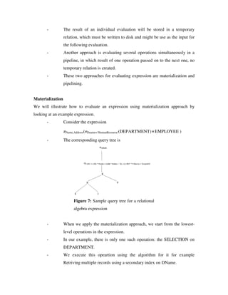
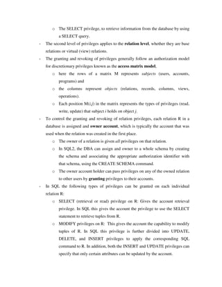
3. SQL Commands Overview – 1
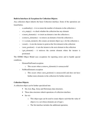
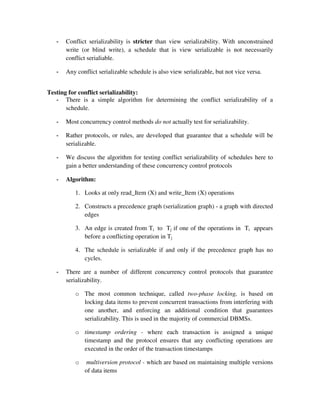
Creating Tables:
Syntax:
CREATE TABLE table_name
(
column1 datatype [constraint],
column2 datatype [constraint],
.
.
columnN datatype [constraint]
);
Example:
Create table student( reg_no number(3) primary key, stud_name varchar2(30),
gender varchar2(6), department varchar2(20), year number);
Describing the structure of the table:
Syntax:
DESC table_name;
Eg:
Desc student;
Populating Tables: (to insert data to the table)
Syntax:
INSERT INTO table_name( column1, column2,…, column)
VALUES (value1, value2, …, valueN);
Eg:
Insert into student values(101, ‘Ahemed’, ‘male’, ‘computer science’,2);
Insert into student(reg_no,stud_name) values(102, ‘John’);
Commit;
Note: commit command helps to make the changes permanent.
Retrieval of Information using SELECT command:
Syntax:
SELECT column1, column2,…,column FROM table1, table2, …, tableN
[WHERE condition] [ORDER BY column [ASC| DESC]];

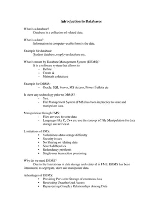
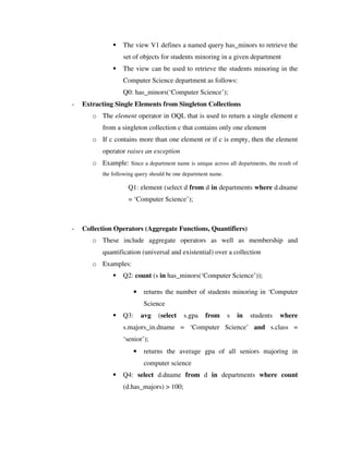
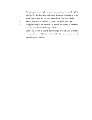
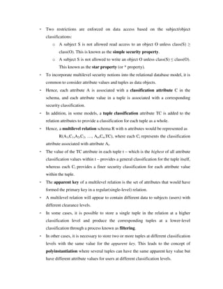
4. Eg:
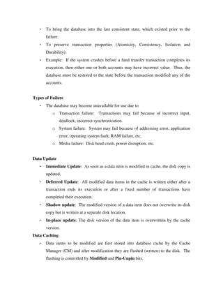
Select reg_no, stud_name from student;
Select stud_name from student where reg_no = 101;
Select * from student;
Select * from student where gender = ‘male’;
Select * from student order by reg_no;
Select * from student where gender = ‘female’ and year = 2;
Select * from student where reg_no > 120;
Select distinct stud_name from student;
Modifying data using UPDATE command:
Syntax:
UPDATE table_name SET column1 = new_value1 [, column2=new_val2, …,
columnN=new_valueN] [WHERE condition];
Eg:
Update student set gender =’male’, department = ‘Mathematics’, year =1
Where reg_no = 102;
Update student set stud_name = ‘Syf Ahemed’ where reg_no = 101;
Deleting data in the table:
Syntax:
DELETE FROM table_name [WHERE condition];
Eg:
Delete from student;
Delete from student where reg_no = 101;
Delete from student where gender = ‘female’ and year =4;
Deleting a table structure using DROP command:
Syntax:
DROP TABLE table_name [CASCADE CONSTRAINTS];
Eg:
Drop table student;
Drop table master cascade constraints;

5. Exercise: 1
1. Create a table named employee with the following fields:
(emp_ID, emp_name, department, designation, qualification, date_of_join, salary)
2. Insert data into the employee table.
3. Retrieve the employee’s details whose highest qualification is doctorate.
4. Find the employee’s name whose salary is greater than 5000 Birrs.
5. Find the employee’s details whose experience is 5 years.
6. Delete the employee’s records who belong to History department.
7. Modify the department name as “Bio-technology” from “Biology”.
8. Increment the salary with 500 Birrs for the employees of “Information
Technology” department.
9. Find the employee’s name whose name start with ‘A’.
10. Find the employees whose department is ‘Administration’ and designation is
‘Computer Operator’.

6. Chapter - 1
OVERVIEW OF OBJECT-ORIENTED CONCEPTS
Introduction
- Traditional databases are used for business database applications. They
have certain shortcomings when more complex database applications
must be designed and implemented.
- For example, databases for engineering design and manufacturing
(CAD/CAM and CIM), scientific experiments, telecommunications,
geographic information systems, and multimedia etc have different
requirements and characteristics.
- They require
Complex structure for objects
Longer-duration transactions
New datatypes for storing images or large textual-items
To define non-standard application-specific operations
- This paved way to the proposal of Object-Oriented Database
Management Systems (OODBMS).
ODBMS
- meets the needs of more complex applications
- gives flexibility (not restricted by datatypes query languages)
- Key Feature: It gives the power to design both structure of complex
objects and their operations.
- it can blend with any Object-Oriented Programming language (OOPL)
- Examples:
for OOPL: SIMULA, SMALL TALK etc.
for hybrid OOPL: C++, JAVA etc.
Features of OODBMS
- An object has two components, namely: value (state) and operations
(behaviour); Objects can be transient or persistent; To make the objects
persistent, we need OODBMS
- OO databases provide a unique system-generated object identifier (OID)
for each object (similar to the concept of primary key)
- Every object structure contains all information that describes the object
(In traditional DB information is scattered over different tables)
- Instance variables hold information that define the internal state of the
object (similar to Attributes or columns in Tables)
- OO models insist that all operations of an object must be predefined.
(complete encapsulation)

7. o For encapsulation, an operation is defined in 2 parts:
• Signature or Interface – to specify operation name
arguments
• Method or Body – to specify implementation of the
operation
o operations can be invoked by passing message
o object structure can be modified without disturbing external programs
o encapsulation provides data-operation independence
- OO systems permits class hierarchies inheritance; this helps for
incremental design and reuse of existing type definitions
- Relationship between objects is made possible by placing the OIDs
within the objects itself and maintaining referential integrity (like
Foreign key constraint)
- Operator polymorphism exists in OODBMS (an operation name
referring to several implementations).
OBJECT IDENTITY, OBJECT STRUCTURE TYPE CONSTRUCTOR
Object Identity (OID)
- It provides a unique identity to each independent object
- OID is system-generated
- Value of OID is not visible to the user
- System uses the OID
o to identify each object and
o to create and manage inter-object references
- The value of OID is immutable (cannot be changed)
- Even if an object is removed from the database, it shall not be assigned to
another object
- OID value cannot depend on any attribute value (since attribute value is liable
to change or correction)
- Sometimes, physical addresses are assigned to OIDs and a hash table is used
to map OID value to physical address.
Object Structure
- Object is identified by a triple, say (OID, type constructor, state)
- Available type constructors are atom, set, tuple and list
Type Constructor
- they are used to define data structures for an OO database schema
- they incorporate the definitions of operations into OO schema

8. - we will use keywords like tuple, set and list for type constructors
- and standard datatypes (like integer, string, float etc) for atomic types.
Encapsulation of operations, methods persistence
- objects can be created, deleted, updated or retrieved or apply calculations
- In database applications, structure of an object is divided into visible and
hidden attributes
- Visible attributes can be directly accessed through high-level query language
- Hidden attributes are completely encapsulated and be accessed only through
pre-defined operations
- Class
o It is an object type definition, along with the definitions and operations
o In the class definition, number of operations are declared
o Implementation of operations are defined elsewhere in the program
o Object Constructor – is to create objects
o Object destructor – is to delete objects
o Object Modifier – is to modify the attribute of an object
o Additional operations are there to retrieve information on objects.
o (eg)
Let Department --- be a class
Let d be the reference object.
Then the operation is represented by dot.
Say, d.no_of_emp ----- is an operation to find the number of
employees in the object d.
And d.dnumber will represent the department number attribute
Persistence
- we can make an object persistent by storing it in the database
- there are 2 mechanisms adapted in OODBMS namely
o Naming
o Reachability
- By Naming mechanism,
o We can give a unique persistent name to the object
o The name can be used to retrieve and manipulate
o But it is not possible to name all the objects, when it is enormous.
- Reachability
o It makes the object reachable from some other persistent object
- hence we can a persistent collection using the Reachability mechanism
- (eg)
o Define a class DEPARTMENT, whose objects are of type,
set(DEPARTMENT)
o Create an object and name it as Alldept (hence it becomes persistent)
o Now any new object is added to the set of Alldept using some
add_dept operation
o Alldept can be called as the EXTENT of the class, as it holds all
persistent objects.

9. TYPE HIERARCHIES AND INHERITANCE
Introduction
- This concept is one other main characteristics of OODBMS
- Type hierarchies imply a constraint on the extents, of the types in hierarchy
- Here both attributes and operations can be inherited.
Why do we need type hierarchies?
- In databases, there are many objects of same type or class
- So classifying objects based on their type becomes mandatory (to be done by
the OODBMS)
- OODBMS should also permit to define new types, based on other pre-defined
types
- This leads to the concept of type (or class) hierarchy.
TYPE Definition:
- A TYPE is defined
o By assigning a type name and
o By defining the attributes and operations
- Attributes and operations can be called as Functions in general (since
attributes resemble functions with zero arguments).
- Syntax for Type Definition
Type_name : function, function, ….., function
- (Eg - 1)
PERSON : Name, IDNo, Address, Birthdate, Age
Note: Here except ‘Age’, all others are attributes. Age is a method.
- (Eg – 2)
EMPLOYEE: Name, IDNo, address, Birthdate, Age, Salary,
Hiredate, Experience
- (Eg - 3)
STUDENT: Name, IDNo, address, Birthdate, Age, Major, GPA
- Subtype
o A Subtype is created when a similar type is to be created
o Subtype inherits all functions of the pre-defined type (called
Supertype)
o (Eg)
EMPLOYEE subtype-of PERSON : Salary, Hiredate, Experience
STUDENT subtype-of PERSON : Major, GPA

10. o EMPLOYEE and STUDENT types can inherit, most of the functions
from PERSON type
o The subtypes can inherit all those implementations too
o Only the functions local or specific to the subtype should be defined
and implemented.
- Hence we find that, a type hierarchy is generated to show the Supertype /
Subtype relationships among all the types declared.
- These Type Definitions
o Describe objects
o They do not generate objects
o It just declares certain types
o As a part of declaration, implementation of functions, of each type is
specified.
- When an object is created, it may belong to one or more existing types
- Each object becomes a member of one or more persistent collection of objects
and it is used to group them together.
Constraints on Extents corresponding to a Type Hierarchy:
- Collection of objects in an EXTENT
o Has the same type or class
o This is applicable to OODBMS
- Each type or subtype will have an Extent associated with it
- The Extent will hold the collection of all persistent objects of that type or
subtype
- Constraint on Extents:
o Every object in an extent of subtype, should also be a member of the
extent of the supertype.
o We can have a ROOT Class (or Object Class), whose extent contains
all objects in the system
o Objects are assigned to additional subtypes, creating a type hierarchy
or class hierarchy.
- Generally in OO Systems, distinction is made between persistent and transient
objects and collections
- Persistent Collection
o Holds a collection of objects stores permanently in the DB
o Can be accessed and shared by multiple programs
- Transient Collection
o It is created during the execution of the program
o But destructed when the program terminates
o Transient collection may be created
In order to hold the result of a query
To collect information from persistent collection and copy to
the transient collection

11. And it can be used by the program only during the execution.
COMPLEX OBJECTS
Introduction
- As we know already, the principal motivation for OO Systems is to
represent complex objects.
- There are two types of complex objects namely
Structured complex objects
Unstructured complex objects
- Structured Complex Objects
It is made up of components
It is defined by applying type constructors recursively at
various levels
- Unstructured Complex Objects
It is a datatype
It requires large amount of storage area
Example: Image or large textual object
Unstructured Complex Objects Type Extensibility:
- It is a facility provided by DBMS to store Unstructured Complex Objects
- The purpose is to store and retrieve large objects
- (Eg) Bitmap images or large text strings
- They are also called as Binary Large Objects (BLOB)
- These objects are called unstructured as
the database does not know what their structure is and
only the application can interpret their meaning
(eg-1) the application may have some functions to display the
image
(eg-2) there may be programs to search keywords in a
document
- these objects are considered to be complex, as they require a large
storage area, beyond the scope of a datatype size
- So object is partially retrieved before loading the whole object
- DBMS uses buffering and caching techniques to prefetch objects
- DBMS cannot process selection conditions or operations based on object
values directly. Only the external program can do the selection.
- This is rectified in OODBMS
By defining a new abstract datatype for un-interpreted object
And by defining methods for selecting, comparing and
displaying objects
- Example:
For retrieving an image object of certain pattern,
• A pattern recognition algorithm is defined as a method

12. • The algorithm is called for an object, to check for its
pattern
- OODBMS also allows to new types with a structure and operations,
which is known as Extensible Type System (Described earlier)
- Applications can use or modify types, by creating subtypes.
- OODBMS provide storage and retrieval of large unstructured objects as
Character strings or Bit strings.
Structured Complex Objects:
- The object structure of Structured Complex Object is defined by the
repeated application of type constructors.
- Example:
Consider the complex object, DEPARTMENT, with
components DNAME, DNO, MGR, LOC, EMP and PROJ.
Here we find that,
• DNAME, DNO : are Basic value attributes
• And the other four are complex valued and builds a
second level of complex object structure.
• MGR : has a tuple structure
• LOC, EMP, PROJ : have set structure
• For MGR tuple, we find two attributes namely,
MGRSTARTDATE – a basic value attribute and
MGRNAME – tuple structure referring to EMP object
• LOC : has a set of basic values
• EMP, PROJ : have sets of tuple structured objects.
Hence we find that the DEPARTMENT complex object is said
to be defined by different type constructors of different levels.
- There are two types of semantics between complex objects and
components at each level namely,
Ownership Semantics
Reference Semantics
- Ownership Semantics:
It applies when components(sub-objects) of complex objects
are encapsulated within the complex object
Those such components are said to have “is-part-of” (or “is-
component-of”) relationship with the complex object
(eg) DNAME, DNO, MGR, LOC from the DEPARTMENT
complex object
These components are considered as a part of internal object
state
They need not have a separate OID
They can only be accessed by methods of the same complex
object
These component objects are deleted when the complex object
is deleted.

13. - Reference Semantics:
It applies when components of the complex object are
independent
Each independent object may have its own identity and
methods
If the complex object, needs to access its referenced
components, it should invoke the methods of the components
(as they are not encapsulated)
Reference Semantics represent relationship among independent
objects
(Ie.)They may be referenced from different complex objects
too
These components shall not be deleted when the complex
object is deleted.
(Eg) EMP, PROJ of DEPARTMENT
They are said to have an “is-associated-with” relationship with
the complex object.
OTHER OBJECT ORIENTED CONCEPTS
POLYMORPHISM:
- Polymorphism of operations is allowed in OODBMS
- OODBMS allows same operator name or symbol
to have 2 or more different implementations
depending upon the type of object, the operator implementation
is applied
- Example:
- Consider a type named GEOMETRY_OBJECT with subtypes namely,
RECTANGLE, TRIANGLE CIRCLE and they are defined as follows:
GEOMETRY_OBJECT: Shape, Area, ReferencePoint
RECTANGLE subtype-of GEOMETRY_OBJECT (Shape = ‘rectangle’):
width, height
TRIANGLE subtype-of GEOMETRY_OBJECT (Shape = ‘triangle’):
Side1, side2, Angle
CIRCLE subtype-of GEOMETRY_OBJECT (Shape = ‘circle’): radius
Consider a method AREA to calculate the area of the GEOMETRY_OBJECT
o then AREA will have a general implementation for calculating area of
any polygon
o Again some efficient algorithms are rewritten to calculate areas of
specific objects

14. o That is, AREA function is overloaded by different implementations.
- OODBMS must select appropriate method for the geometric object applied to.
- Selection is made in 2 ways, namely
Compile-time selection – during compilation. Also known as
Static Binding.
Run-time selection – during execution. Also known as
Dynamic Binding.
MULTIPLE INHERITANCES:
- Multiple inheritance occurs when a subtype is a subtype of two or more types
and it inherits functions from both the supertypes
- It leads to a creation of type lattice.
- (eg) ENGINEERING_MANAGER
It is a subtype of MANAGER and ENGINEER types.
- There exits a problem, when supertypes having distinct functions are inherited
by the subtypes
- Ambiguity is caused by the names (being the same) of the functions
- If the function name and its implementation are quite the same, then the
problem is eliminated by inheriting only one function.
- If the implementation differs, then one of the following steps can be taken:
o The system can allow the user to select one among the functions from
the supertypes
o Or setting one among the functions as default
o Or disallowing multiple inheritance, when name ambiguity occurs.
o Or forcing the user to change the name of the function.
SELECTIVE INHERITANCE:
- this occurs when a subtype
inherits only some functions of the supertype and
other functions are not inherited
- then an EXCEPT clause is used to list down the functions eliminated from
deriving from the supertype
- this is not much used in OO Systems except other than Artificial Intelligence
Systems.

15. Chapter - 2
OBJECT MODEL OF ODMG
ODMG Object Model:
- Just like Relational Model, we have the ODMG Object Data Model upon
which ODL and OQL are based.
- This object model provides facilities to define data types, use type
constructors and also concepts to specify object database schemas.
Objects and Literals:
- Objects and Literals are the basic building blocks of the object model.
- An object has an object identifier and state.
- A Literal has only the value, which will be a constant; it can be complex too.
- An object value or literal value can have a complex structure.
- An object state is liable to change overtime, by the modification of object
value.
- An object is described by four characteristics:
o Identifier
It is the Object Identifier, which is a unique system-wide
identifier.
o Name
Some objects may optionally have a unique name
The name is used to refer objects
Extents will have a name, which is used as an entry point to
database.
o Life time
Life time specifies whether the object is transient or persistent.
o Structure
The structure specifies how the object is constructed by using
type constructors

16. It also specifies whether the object is atomic or a collection
object.
- there are three types of literals, which are described as follows:
o Atomic Literal
Here the values are of basic or pre-defined datatypes
Datatype can be one among the following: long, short,
unsigned long, unsigned short, float, double, Boolean, char,
string, enum etc.
o Collection Literal
It can be a collection of objects or values
But it will not have an OID.
o Structured Literal
These are values roughly constructed values using tuple
constructors
They are user-defined structures constructed using “struct”
keyword
(Eg) – Date, Interval, Time, Time Stamp etc
Built-in Interfaces:
- In Object Model, all objects inherit the basic interface of object.
- Some basic operations are listed below:
o COPY
Creates a new copy of the object
(Eg) Let o and p be two objects.
Then, p = o.copy(), where value of o is copied to p.
o DELETE
This is used to delete an object
To delete the object o, we can write o.delete()
o SAME AS
This is to compare OID of an object with the other.
To compare the objects o and p, o.same_as(p)

17. Built-in Interfaces Execptions for Collection Objects:
Any collection object inherits the basic Collection interface. Some of the operations are
listed below.
- o.cardinality() – it is to return the number of elements in the collection o
- o.is_empty() – to check whether the collection has any element
- o.insert_element(e) – to insert an element e into the collection o.
- o.remove_element(e) – to remove an element e from the collection o.
- i = o.create_iterator(), this creates an iterator object say i, for the collection o.
- i.reset() - it sets the iterator to point at the first element in the collection
- i.next_position() – it sets the iterator to the next element in the collection
- i.get_element() – it retrieves the current element where the iterator is
positioned.
The ODMG Object Model uses exceptions for reporting errors and to handle special
conditions.
- ElementNotFound exception
o This occurs when o.remove_element(e) is unsuccessful
- NoMoreElements exception
o This occurs when i.next_position() is unsuccessful and does not have
further more elements in the collection for further retrieval.
Collection Objects:
A collection object can be further specialized into
• Set, List, Bag, Array and Dictionary data structures.
• These data structures inherit operations of collection interface.
• Set t
o This object type can be used to create objects such that the value of
object o is a set whose elements are of type t.
o The Set interface includes the additional operation,

18. o p = o.create_union(s), which returns a new object p of type Sett
that is the union of the two sets o and s
o create_intersection(s), create_difference(s) are also some other
operations like create_union.
o Operations for set comparison include the o.is_subset_of(s)
operation, which returns true if the set object o is a subset of some
other set object s, and returns false otherwise. Similar operations
are is_proper_subset_of(s), is_superset_of(s), and
is_proper_superset_of(s).
• The Bagt object type allows duplicate elements in the collection and
also inherits the Collection interface.
o It has three operations—create_union(b), create_intersection(b),
and create_difference(b)—that all return a new object of type
Bagt.
o For example, p = o.create_union(b) returns a Bag object p that is
the union of o and b (keeping duplicates).
o The o.occurrences_of(e) operation returns the number of duplicate
occurrences of element e in bag o
• A Listt can be used to create collections where the order of the
elements is important. The value of each such object o is an ordered list
whose elements are of type t. Hence, we can refer to the first, last, and ith
element in the list.
o If o is an object of type Listt, the operation
o.insert_element_first(e) inserts the element e before the first
element in the list o, so that e becomes the first element in the list.
o Similar operations are o.insert_element_last(e),
o.insert_element_after(e,i)and o.insert_element_before(e,i),
o To remove elements from the list, the operations are e =
o.remove_first_element(), e = o.remove_last_element(), and e =
o.remove_element_at(i)

19. o To retrieve elements, e = o.retrieve_first_element(), e =
o.retrieve_last_element(), and e = o.retrieve_element_at(i).
• The Arrayt object type also inherits the Collection operations. It is
similar to a list except that an array has a fixed number of elements.
o The specific operations for an Array object o are
o.replace_element_at(i,e), which replaces the array element at
position i with element e; e = o.remove_element_at(i), which
retrieves the ith element and replaces it with a null value; and e =
o.retrieve_element_at(i), which simply retrieves the ith element of
the array.
o Any of these operations can raise the exception InvalidIndex if i is
greater than the array’s size.
o The operation o.resize(n) changes the number of array elements to
n..
• The last type of collection objects are of type Dictionaryk, v. This
allows the creation of a collection of association pairs k, v, where all k
(key) values are unique. This allows for associative retrieval of a particular
pair given its key value (similar to an index).
o If o is a collection object of type Dictionaryk,v, then o.bind(k,v)
binds value v to the key k as an association k,v in the collection,
whereas o.unbind(k) removes the association with key k from o
o v = o.lookup(k) returns the value v associated with key k in o.
o The latter two operations can raise the exception KeyNotFound.
Finally, o.contains_key(k) returns true if key k exists in o, and
returns false –otherwise.
Atomic Objects
o In the object model, any user-defined object that is not a collection object is called
an atomic object.

20. o For example, in a UNIVERSITY database application, the user can specify an
object type (class) for Student objects. Most such objects will be structured
objects;
o for example, a Student object will have a complex structure, with many attributes,
relationships, and operations, but it is still considered atomic because it is not a
collection. Such a user-defined atomic object type is defined as a class by
specifying its properties and operations. The properties define the state of the
object and are further distinguished into attributes and relationships.
Interfaces, Classes and Inheritance
o In the ODMG 2.0 object model, two concepts exist for specifying object types:
interfaces and classes and there are two types of inheritance relationships existing.
o An interface is a specification of the abstract behavior of an object type, which
specifies the operation signatures. Although an interface may have state properties
(attributes and relationships) as part of its specifications, these cannot be inherited
from the interface, as we shall see. An interface also is noninstantiable—that is,
one cannot create objects that correspond to an interface definition.
o A class is a specification of both the abstract behavior and abstract state of an
object type, and is instantiable—that is, one can create individual object
instances corresponding to a class definition.
o Because interfaces are noninstantiable, they are mainly used to specify abstract
operations that can be inherited by classes or by other interfaces. This is called
behavior inheritance and is specified by the : symbol . Hence, in the ODMG
2.0 object model, behavior inheritance requires the supertype to be an interface,
whereas the subtype could be either a class or another interface.
o Another inheritance relationship, called EXTENDS and specified by the extends
keyword, is used to inherit both state and behavior strictly among classes. In an
EXTENDS inheritance, both the supertype and the subtype must be classes.
Multiple inheritance via EXTENDS is not permitted. However, multiple
inheritance is allowed for behavior inheritance via :. Hence, an interface may
inherit behavior from several other interfaces. A class may also inherit behavior

21. from several interfaces via :, in addition to inheriting behavior and state from at
most one other class via EXTENDS.
Extents, Keys and Factory Objects:
• Extent:
The database designer can declare an extent for any object type
that is defined via a class declaration.
The extent is given a name, and it will contain all persistent objects
of that class.
Hence, the extent behaves as a set object that holds all persistent
objects of the class.
Extents are also used to automatically enforce the set/subset
relationship between the extents of a supertype and its subtype
For Example, the Employee and Department classes have extents
called all_employees and all_departments, respectively.
• Keys:
A class with an extent can have one or more keys.
A key consists of one or more properties (attributes or
relationships) whose values are constrained to be unique for each
object in the extent.
For example, the Employee class has the EmployeeID attribute as
key and the Department class has two distinct keys: dname and
dnumber.
• Factory Objects:
It is the object that can be used to generate or create individual
objects via its operations
For example, DateObject can have additional operations like
calendar_date, for creating some more objects based on that. (Say
different operations on the calendar and creating different calendar
types).

22. ODL and OQL
The Object Definition Language
- The ODL is designed to support the semantic constructs of the ODMG object
model
- ODL is independent of any particular programming language.
- Its main use is to create object specifications—that is, classes and interfaces.
- Hence, ODL is not a full programming language.
- ODL constructs can be used in programming languages (like C++, JAVA etc)
- Example:
o Let us consider an interface GeometryObject with operations to
calculate the perimeter and area of a geometric object.
o Several classes (Rectangle, Triangle, Circle, etc) inherit the
GeometryObject interface.
o Since GeometryObject is an interface, it is noninstantiable—that is, no
objects can be created based on this interface directly.
o However, objects of type Rectangle, Triangle, Circle, etc. can be
created, and these objects inherit all the operations of the
GeometryObject interface.
o The inherited operations can have different implementations in each
class.
o For example, the implementations of the area and perimeter operations
may be different for Rectangle, Triangle, and Circle.
- Multiple inheritance of interfaces by a class is allowed, as is multiple
inheritance of interfaces by another interface.
- However, a class can inherit via EXTENDS from at most only one class
The Object Query Language (OQL):

23. - OQL is the query language proposed for the ODMG object model.
- It is designed to work closely with the programming languages for which an
ODMG binding is defined, such as C++, SMALLTALK, and JAVA.
- Hence, an OQL query can be embedded into one of these programming
languages.
- The OQL syntax for queries is similar to the syntax of the relational standard
query language SQL, with additional features for ODMG concepts, such as
object identity, complex objects, operations, inheritance, polymorphism, and
relationships.
- The basic OQL syntax is a select . . . from . . . where . . . structure, as for
SQL.
- For example, the query to retrieve the names of all departments in the college
of ‘Engineering’ can be written as follows:
Q0: Select d.dname from d in departments where
d.college=’Engineering’;
- For queries in general, the entry point to the database is the name of the extent
of a class.
- Here the named object departments is of type setDepartment
- Whenever a collection is referenced in an OQL query, we should define an
iterator variable —d in Q0—that ranges over each object in the collection.
- In Q0, only persistent objects d in the collection of departments that satisfy the
condition d.college = ‘Engineering’ are selected for the query result.
- For each selected object d, the value of d.dname is retrieved in the query
result.
- There are three syntactic options for specifying iterator variables:
o d in departments
o departments d
o departments as d

24. - A query does not have to follow the select . . . from . . . where . . . structure.
It can simply be called by the extent name as follows:
Q1: departments;
Q1a: csdepartment;
- Here persistent names like departments is given to a collection of all persistent
department objects, whose type is setDepartment and csdepartment is given
to a single department object say computer science department object
respectively.
- Path Expressions
o Once an entry point is specified, the concept of a path expression can
be used to specify a path to related attributes and objects.
o A path expression typically starts at a persistent object name, or at the
iterator variable that ranges over individual objects in a collection.
o This name will be followed by zero or more relationship names or
attribute names connected using the dot notation.
o Some examples are given as follows:
Q2: csdepartment.chair;
• Q2 returns a Faculty object that is related to the
department object whose persistent name is
csdepartment via the attribute chair; that is, the
chairperson of the computer science department is
retrieved.
Q2a: csdepartment.chair.rank;
• it returns the rank of this chair person
• the attributes chair (of Department) and rank (of
Faculty) are both single-valued and they are applied to
a single object.
Q2b: csdepartment.has_faculty;
• It returns a collection which includes all Faculty objects
that are related to the department object whose

25. persistent name is csdepartment via the relationship
has_faculty; that is, all Faculty objects who are working
in the computer science department are retrieved.
But we cannot write as follows:
Q3’: csdepartment.has_faculty.rank;
• This is because it is not clear whether the object
returned would be of type setstring or bagstring
(the latter being more likely, since multiple faculty may
share the same rank).
• Because of this type of ambiguity problem, OQL does
not allow expressions such as Q3’.
• Rather, one must use an iterator variable over these
collections, as in Q3 below:
Q3: Select distinct f.rank from f in
csdepartment.has_faculty;
- In general, an OQL query can return a result with a complex structure
specified in the query itself by utilizing the struct keyword.
- Some examples are as follows:
o Q4: select struct(deg: d.degree, yr: d.years, college: d.college)
from d in degrees;
The degrees component is a collection of three string
components: deg, yr, and college
o Q5: csdepartment.chair.advises;
This is the collection of graduate students that are advised by
the chair of the computer science department.
We can have a still more complexive query as follows:
o Q6: Select struct (name:struct(last_name: s.name.lname,
first_name: s.name.fname), degrees:(select struct (deg:

26. d.degree, yr: d.year, college: d.college) from d in
s.degrees) from s in csdepartment.chair.advises;
the result is a collection of (first-level) structs where each struct
has two components: name and degrees
The name component is a further struct made up of last_name
and first_name, each being a single string.
The degrees component is defined by an embedded query and
is itself a collection
o Q7: select struct (last_name: s.name.lname, first_name:
s.name.fname, gpa: s.gpa) from s in students where
s.majors_in.dname = ‘Computer Science’ and s.class = ‘senior’ order
by gpa desc, last_name asc, first_name asc;
The query retrieves the grade point average of all senior
students majoring in computer science, with the result ordered
by gpa, and within that by last and first name.
Other Features of OQL:
- Specifying Views as Named Queries
o The view mechanism in OQL uses the concept of a named query.
o The define keyword is used to specify an identifier of the named
query, which must be a unique name among all named objects, class
names, method names, or function names in the schema.
o If the identifier has the same name as an existing named query, then
the new definition replaces the previous definition.
o Once defined, a query definition is persistent until it is redefined or
deleted.
o A view can also have parameters (arguments) in its definition.
o Example:
V1: define has_minors(deptname) as select s from s in students
where s.minors_in.dname = deptname;

27. The view V1 defines a named query has_minors to retrieve the
set of objects for students minoring in a given department
The view can be used to retrieve the students minoring in the
Computer Science department as follows:
Q0: has_minors(‘Computer Science’);
- Extracting Single Elements from Singleton Collections
o The element operator in OQL that is used to return a single element e
from a singleton collection c that contains only one element
o If c contains more than one element or if c is empty, then the element
operator raises an exception
o Example: Since a department name is unique across all departments, the result of
the following query should be one department name.
Q1: element (select d from d in departments where d.dname
= ‘Computer Science’);
- Collection Operators (Aggregate Functions, Quantifiers)
o These include aggregate operators as well as membership and
quantification (universal and existential) over a collection
o Examples:
Q2: count (s in has_minors(‘Computer Science’));
• returns the number of students minoring in ‘Computer
Science
Q3: avg (select s.gpa from s in students where
s.majors_in.dname = ‘Computer Science’ and s.class =
‘senior’);
• returns the average gpa of all seniors majoring in
computer science
Q4: select d.dname from d in departments where count
(d.has_majors) 100;

28. • retrieves all department names that have more that 100
majors
Q5: Jeremy in has_minors(‘Computer Science’);
• The query answers the following question: Is Jeremy a
computer science minor?
Q6: for all g in (select s from s in grad_students where
s.majors_in.dname = ‘Computer Science’) : g.advisor in
csdepartment.has_faculty ;
• Thus answers the question Are all computer science
graduate students advised by computer science
faculty?”
Q7: exists g in (select s from s in grad_students where
s.majors_in.dname = ‘Computer Science’) : g.gpa = 4;
• This answers the question: Does any graduate
computer science major have a 4.0 gpa?
- Ordered (Indexed) Collection Expressions
o Operations exist for extracting a subcollection and concatenating two
lists.
o A sample is given in the following example
Q8: first(select struct(faculty: f.name.lname, salary:
f.salary) from f in faculty order by f.salary desc);
o It retrieves the last name of the faculty member who earns the highest
salary
- The Grouping Operator
o The group by clause in OQL, although similar to the corresponding
clause in SQL, provides explicit reference to the collection of objects
within each group or partition.

29. o Q9 retrieves the number of majors in each department. In this query,
the students are grouped into the same partition (group) if they have
the same major; that is, the same value for s.majors_in.dname
Q9: select struct(deptname, number_of_majors: count
(partition)) from s in students group by deptname:
s.majors_in.dname;
o Q10 retrieves for each department having more than 100 majors, the
average gpa of its majors. The having clause in Q10 selects only those
partitions (groups) that have more than 100 elements (that is,
departments with more than 100 students).
Q10: select deptname, avg_gpa: avg (select p.s.gpa from p in
partition) from s in students group by deptname:
s.majors_in.dname having count(partition)100;

30. Chapter – 3
Object-Relational Features of Oracle 8
Introduction
- Here we will review a number of features related to the version of the Oracle
DBMS product called Release 8.X, which has been enhanced to incorporate
object-relational features.
- A number of additional data types with related manipulation facilities called
cartridges have been added.
- For example, the spatial cartridge allows map-based and geographic
information to be handled
- Management of multimedia data has also been facilitated with new data types
- As an ORDBMS, Oracle 8 continues to provide the capabilities of an RDBMS
and additionally supports object-oriented concepts.
- Application developers can manipulate application objects as opposed to
constructing the objects from relational data.
- The complex information about an object can be hidden, but the properties
(attributes, relationships) and methods (operations) of the object can be
identified in the data model
- Object type declarations can be reused via inheritance, thereby reducing
application development time and effort.
Defining Types
- Oracle allows us to define types similar to the types of SQL.
- The syntax is
CREATE TYPE type_name AS OBJECT (
list of attributes and methods
);
- For example here is a definition of a point type consisting of two numbers:
CREATE TYPE PointType AS OBJECT (x NUMBER(2),
y NUMBER(2));

31. - An object type can be used like any other type in further declarations of
object-types (subtypes) or table-types. For instance, we might define a line
type by:
CREATE TYPE LineType AS OBJECT (
end1 PointType, end2 PointType);
- Then, we could create a relation (which uses the LineType) that is a set of lines
with ``line ID's'' as:
CREATE TABLE Lines (lineID INT, line LineType);
- Insertion of values for the objects is also possible as follows:
INSERT INTO Lines VALUES ( 27,
LineType( PointType(0, 0), PointType(3, 4)));
- The following query prints the x and y coordinates of the first end of each line.
Here “l1” is the iterator for the table “Lines” and path expression is used for
manipulating column values.
SELECT ll.line.end1.x, ll.line.end1.y FROM Lines ll;
- The following query prints the second end of each line, but as a value of type
PointType, not as a pair of numbers. For instance, one line of output would
be PointType(3,4). Notice that type constructors are used for output as well
as for input.
SELECT ll.line.end2 FROM Lines ll;
- Update and Delete operations are also possible like ordinary SQL queries.
Update Lines L set L.line.end1.x = 5, L.line.end1.y = 6
where lineID= 2;
Delete from Lines L where L.line.end2.x=3 and L.line.end2.y=4;
- Dropping Types: To get rid of a type such as LineType, we say:
DROP TYPE Linetype;

32. - However, before dropping a type, we must first drop all tables and other
types that use this type. Thus, the above would fail because table Lines still
exists and uses LineType.
Representing Multivalued Attributes Using VARRAY
- Some attributes of an object/entity could be multivalued.
- Here all the attributes of an object—including multivalued ones—are
encapsulated within the object
- Oracle 8 achieves this by using a varying length array (VARRAY) data type,
which is user-defined.
Examples:
- Consider the example of a customer VARRAY entity with attributes name
and phone_numbers, where phone_numbers is multivalued.
- First, we need to define an object type representing a phone_number as
follows:
CREATE TYPE phone_num_type AS OBJECT (phone_number CHAR(10));
- Then we define a VARRAY whose elements would be objects of type
phone_num_type:
CREATE TYPE phone_list_type as VARRAY (5) OF phone_num_type;
- Now we can create the customer_type data type as an object with attributes
customer_name and phone_numbers:
CREATE TYPE customer_type AS OBJECT (customer_name VARCHAR(20),
phone_numbers phone_list_type);
- It is now possible to create the customer table as
CREATE TABLE customer OF customer_type;
- To retrieve a list of all customers and their phone numbers, we can issue a
simple query without any joins:
SELECT customer_name, phone_numbers FROM customers;
Using Nested Tables to Represent Complex Objects
- In object modeling, some attributes of an object could be objects themselves.

33. - Oracle 8 accomplishes this by having nested tables
- Here, columns (equivalent to object attributes) can be declared as tables.
- Nested tables are like a single column database table; no limit on size; not
ordered
Examples:
- In the above example let us assume that we have a description attached to
every phone number (for example, home, office, cellular). This could be
modeled using a nested table by first redefining phone_num_type as follows:
CREATE TYPE phone_num_type AS OBJECT (phone_number CHAR(10),
description CHAR(30));
- We next redefine phone_list_type as a table of phone_number_type as
follows:
CREATE TYPE phone_list_type AS TABLE OF phone_number_type;
- We can then create the type customer_type and the customer table as before.
The only difference is that phone_list_type is now a nested table instead of a
VARRAY. Both structures have similar functions with a few differences.
- Let us see another example below:
create or replace type supplier as table of char(3);
create table product
(prodno char(5) primary key, price number(5,2), supplierno supplier)
nested table supplierno store as supplier_tbl;
insert into product values ('XYZ01', 23.45, supplier('101','224', '456'));
insert into product values ('XYZ02', 42.56, supplier('224','572'));

34. - Here, the supplier type code creates a nested table containing supplier
numbers. The product table created above contains the supplier table as a
nested table. The nested table clause specifies a table name for the supplier
data; unlike a VARRAY, a nested table is stored in a separate table. The
SUPPLIER constructor function is used when a row is added to the
PRODUCT table.
Similarities and Differences between VARRAY and Nested Tables:
o Nested tables do not have an upper bound on the number of items whereas
VARRAYs do have a limit.
o Individual items can be retrieved from the nested tables, but this is not
possible with VARRAYs.
o Additional indexes can also be built on nested tables for faster data access.
Managing Large Objects and Other Storage Features
- Oracle can now store extremely large objects like video, audio, and text
documents.
- New data types have been introduced for this purpose.
- These include the following:
1. BLOB (binary large object).
2. CLOB (character large object).
3. BFILE (binary file stored outside the database).
4. NCLOB (fixed-width multibyte CLOB).

35. - All of the above except for BFILE, which is stored outside the database, are
stored inside the database along with other data.
- Only the directory name for a BFILE is stored in the database.
Index Only Tables
- Oracle 8 supports both the standard indexing scheme and also index only
tables
- In Index only tables, the data records and index are kept together in a B-tree
structure
- This allows faster data retrieval and requires less storage space for small-to
medium-sized files where the record size is not too large.
Partitioned Tables and Indexes
Large tables and indexes can be broken down into smaller partitions. The table now
becomes a logical structure and the partitions become the actual physical structures that
hold the data. This gives the following advantages:
• Continued data availability in the event of partial failures of some partitions.
• Scalable performance allowing substantial growth in data volumes.
• Overall performance improvement in query and transaction processing
Implementation and Related Issues for Extended Type Systems
- There are various implementation issues regarding the support of an extended
type system with associated functions (operations). They are summarized below:
o The ORDBMS must dynamically link a user-defined function in its
address space only when it is required.
Numerous functions are required to operate on two-or three-
dimensional spatial data, images, text, and so on.
With a static linking of all function libraries, the DBMS address
space may increase by an order of magnitude.
Therefore dynamic linking is adapted in ORDBMS.
o Client-server issues deal with the placement and activation of functions.

36. If the server needs to perform a function, it is best to do so in the
DBMS address space rather than remotely, due to the large amount
of overhead.
For security reasons, it is better to run functions at the client using
the user ID of the client.
Functions are likely to be written in interpreted languages like
JAVA.
o It should be possible to run queries inside functions.
A function must operate the same way whether it is used from an
application using the application program interface (API), or
whether it is invoked by the DBMS as a part of executing SQL
with the function embedded in an SQL statement.
Systems should support a nesting of these callbacks.
o Because of the variety in the data types in an ORDBMS and associated
operators, efficient storage and access of the data is important
For spatial data or multidimensional data, new storage structures
such as R-trees, quad trees, or Grid files may be used.
The ORDBMS allows new types to be defined with new access
structures.
Dealing with large text strings or binary files also opens up a
number of storage and search options.

37. Chapter – 4 QUERY PROCESSING
Introduction
- Query processing is a set of activities involving in getting the result of a
query expressed in a high-level language.
- These activities includes parsing the queries and translate them into
expressions that can be implemented at the physical level of the file
system, optimizing the query of internal form to get a suitable execution
strategies for processing and then doing the actual execution of queries
to get the results.
- The cost of processing of query is dominated by the disk access.
- For a given query, there are several possible strategies for processing
exist, especially when query is complex. The difference between a good
strategies and a bad one may be several order of magnitude. Therefore, it
is worthwhile for the system to spend some time on selecting a good
strategies for processing query.
1. Overview of Query Processing
- Here we discuss the techniques used by a DBMS to process, optimize,
and execute high-level queries.
- A query expressed in a high-level query language such as SQL must first
be scanned, parsed, and validated.
The scanner identifies the language tokens—such as SQL
keywords, attribute names, and relation names—in the text of the
query
Whereas the parser checks the query syntax to determine whether
it is formulated according to the syntax rules (rules of grammar) of
the query language.

38. The query must also be validated, by checking that all attribute and
relation names are valid and semantically meaningful names in the
schema of the particular database being queried.
- The main steps in processing a high-level query are illustrated in the
following figure.
Figure 1: Steps in query processing process
- An internal representation of the query is then created, usually as a tree
data structure called a query tree.
- It is also possible to represent the query using a graph data structure
called a query graph.
- The DBMS must then devise an execution strategy for retrieving the
result of the query from the database files.
- A query typically has many possible execution strategies, and the
process of choosing a suitable one for processing a query is known as
query optimization.
- The query optimizer module has the task of producing an execution plan,
and the code generator generates the code to execute that plan.

39. - The runtime database processor has the task of running the query code,
whether in compiled or interpreted mode, to produce the query result. If
a runtime error results, an error message is generated by the runtime
database processor.
- The functions of Query Parser is parsing and translating a given high-
leval language query into its immediate form such as relational algebra
expressions.
- A relational algebra expression of a query specifies only partially how to
evaluate a query, there are several ways to evaluate an relational algebra
expression.
- For example, consider the query :
SELECT Salary FROM EMPLOYEE WHERE Salary = 50,000 ;
- The possible relational algebra expressions for this query are:
• ΠSalary(σSalary=50000(EMPLOYEE))
• σSalary=50000(ΠSalaryEMPLOYEE)
(OR)
• PSalary(SSalary=50000(EMPLOYEE))
• SSalary=50000(PSalaryEMPLOYEE)
- In order to specify fully how to evaluate a query, the system is
responsible for constructing a query execution plan which made up of
the relational algebra expression and the detailed algorithms to evaluate
each operation in that expression.
- Moreover, the selected plan should minimize the cost of query
evaluation. The process of choosing a suitable query execution plan is
known as query optimization. This process is perform by Query
Optimizer.
- Once the query plan is chosen, the Query Execution Engine lastly take
the plan, executes that plan and return the answer of the query.

40. - In the following sections, we give an overview of query optimization
techniques.
The first one based on heuristic rules for ordering operations in
the query execution plan.
The second technique involves estimating the cost of different
execution plan based on the systematic information.
Most of the commercial DBMS’s query optimizers use the
combination of these two methods.
2. Using Heuristic in Query Optimization
Heuristic optimization applies the rules to the initial query expression and
produces the heuristically transformed query expressions.
- A heuristic is a rule that works well in most cases but not always
guaranteed. For example, a rule for transforming relational-algebra
expression is “Perform selection operations as early as possible”.
- This rule is generate based on intuitive idea that selection is the
operation that results a subset of the input relation so apply selection
early might reduce the immediate result size.
- However, there are cases perform selection before join is not a good
idea.
- In this section, we firstly introduce how the heuristic rules can be used to
convert a initial query expression to an equivalent one then we discuss
the generation of query execution plan.
2.1 Transformation of Relational Expression
- One aspect of optimization occurs at relational algebra level.
- This involves transforming an initial expression (tree) into an equivalent
expression (tree) which is more efficient to execute.
- Two relational algebra expressions are said to be equivalent if the two
expressions generate two relation of the same set of attributes and

41. contain the same set of tuples although their attributes may be ordered
differently.
- The query tree is a data structure that represents the relational algebra
expression in the query optimization process.
- The leaf nodes in the query tree correspond to the input relations of the
query.
- The internal nodes represent the operators in the query.
- When executing the query, the system will execute an internal node
operation whenever its operands available, then the internal node is
replaced by the relation which is obtained from the preceding execution.
2.1.1 Equivalence Rules for transforming relational expressions
There are many rules which can be used to transform relational algebra operations to
equivalent ones. We will state here some useful rules for query optimization.
In this section, we use the following notation:
• E1, E2, E3,… : denote relational algebra expressions
• X, Y, Z : denote set of attributes
• F, F1, F2, F3 ,… : denote predicates (selection or join conditions)
• Commutativity of Join, Cartesian Product operations
• Natural Join operator is a special case of Join, so Natuaral Joins are also
commutative.
• Associativity of Join , Cartesian Product operations
(E1∗E2)∗E3 ≡E1∗( E2∗E3)
(E1×E2)×E3≡E1×( E2×E3)
(E1F1E2)F2E3≡E1F1(E2F2E3)
- Join operation associative in the following manner: F1 involves attributes
from only E1 and E2 and F2 involves only attributes from E2 and E3

42. • Cascade of Projection
PX1(PX2(...(PXn(E))...))≡ PX1 (E)
• Cascade of Selection
SF1∧F2∧...∧Fn(E)≡ SF1 (SF2(...(SFn(E))...))
• Commutativity of Selection
SF1(SF2(E))≡ SF2 (SF1(E))
• Commuting Selection with Projection
PX(SF(E))≡SF (PX(E))
(This rule holds if the selection condition F involves only the attributes in set X.)
• Selection with Cartesian Product and Join
• If all the attributes in the selection condition F involve only the
attributes of one of the expression say E1, then the selection and Join
can be combined as follows:
SF(E1CE2)≡(SF(E1))CE2
• If the selection condition F = F1 AND F2 where F1 involves only
attributes of expression E1 and F2 involves only attribute of
expression E2 then we have:
SF1∧F2(E1CE2)≡( SF1(E1))C(SF2(E2))
• If the selection condition F = F1 AND F2 where F1 involves only
attributes of expression E1 and F2 involves attributes from both E1
and E2 then we have:
SF1∧F2(E1CE2)≡SF2 ((SF1(E1))CE2)
The same rule apply if the Join operation replaced by a Cartersian
Product operation.
• Commuting Projection with Join and Cartesian Product
• Let X, Y be the set of attributes of E1 and E2 respectively. If the join
condition involves only attributes in XY (union of two sets) then :
PXY(E1FE2)≡PX (E1)FPY(E2)
The same rule apply when replace the Join by Cartersian Product.

43. • If the join condition involves additional attributes say Z of E1 and W
of E2 and Z,W are not in XY then :
PXY(E1FE2)≡PXY (πXZ(E1)FPYW(E2))
• Commuting Selection with set operations
The Selection commutes with all three set operations (Union, Intersect,
Set Difference) .
SF(E1∧E2)≡( SF(E1))∧( SF(E2))
The same rule apply when replace Union by Intersection or Set
Difference
• Commuting Projection with Union
PX(E1∧E2)≡( PX(E1))∧( PX(E2))
• Commutativity of set operations: The Union and Intersection are commutative but
Set Difference is not.
E1∧E2≡E2∧E1
E1∩E2≡E2∩E1
• Associativity of set operations: Union and Intersection are associative but Set
Difference is not
(E1∧E2)∧E3 ≡E1∧( E2∧E3)
(E1∩E2)∩E3 ≡E1∩( E2∩E3)
• Converting a Catersian Product followed by a Selection into Join.
If the selection condition corresponds to a join condition we can do the
convert as follows:
SF(E1×E2)≡E1 FE2

44. 2.1.2 Example of Transformation
Consider the following query on COMPANY database: “Find the name of employee born
after 1967 who work on a project named ‘Greenlife’ “.
The SQL query is:
SELECT Name FROM EMPLOYEE E, JOIN J, PROJECT P
WHERE E.EID = J.EID and PCode = Code and
Bdate ’31-12-1967’ and P.Name = ‘Greenlife’;
The initial query tree for this SQL query is
Figure 2: Initial query tree for query in example
We can transform the query in the following steps:
- Using transformation rule, apply on Catersian Product and Selection
operations to moves some Selection down the tree.
- Selection operations can help reduce the size of the temprary relations which
involve in Catersian Product.

45. Figure 3: Move Selection down the tree
- Using the rule to convert the sequence (Selection, Cartesian Product) in
to a Join. In this situation, since the Join condition is equality
comparison in same attributes so we can convert it to Natural Join.
Figure 4: Combine Catersian Product with subsequent
Selection into Join
- Using rule move Projection operations down the tree.

46. Figure 5: Move projections down the query tree
2.2 Heuristic Algebraic Optimization algorithm
Here are the steps of an algorithm that utilizes equivalence rules to transfrom the query
tree.
• Break up any Selection operation with conjunctive conditions into a cascade of
Selection operations.
• Move selection operations as far down the query tree as possible. This step use
the commutativity and associativity of selection.
• Rearrange the leaf nodes of the tree so most restrictive selections are done first.
o Most restrictive selection is the one that produces the fewest number of
tuples.
o In addition, make sure that the ordering of leaf nodes does not cause the
Catersian Product operation.
o This step relies on the rules of associativity of binary operations.
• Combine a Cartesian Product with a subsequent Selection operation into a Join
operation if the selection condition represents a join condition
• Break down and move lists of projection down the tree as far as possible, creating
new Projection operations as needed.
• Identify sub-tree that present groups of operations that can be pipelined and
executing them using pipelining.
The previous example illustrates the transforming of a query tree using this algorithm.

47. 2.3 Converting query tree to query evaluation plan
- Query optimizers use the above equivalence rules to generate a
enumeration of logically equivalent expressions to the given query
expression.
- However, expression generating is just one part of the optimization
process.
- As mentioned above, the evaluation plan includes the detail algorithm
for each operation in the expression and how the execution of the
operations is coordinated.
- The figure shows an evaluation plan.
Figure 6: An evaluation plan
- As we know, the output of Parsing and Translating step in the query
processing is a relational algebra expression.
- For a complex query, this expression consists of several operations and
interact with various relations.
- Thus the evaluation of the expression is very costly in terms of both time
and memory space.
- Now we consider how to evaluate an expression containing multiple
operations.
- The obvious way to evaluate the expression is simply evaluate one
operations at a time in an appropriate order.

48. - The result of an individual evaluation will be stored in a temporary
relation, which must be written to disk and might be use as the input for
the following evaluation.
- Another approach is evaluating several operations simultaneously in a
pipeline, in which result of one operation passed on to the next one, no
temporary relation is created.
- These two approaches for evaluating expression are materialization and
pipelining.
Materialization
We will illustrate how to evaluate an expression using materialization approach by
looking at an example expression.
- Consider the expression
πName,Address(σDname='HumanResourse'(DEPARTMENT)∗EMPLOYEE )
- The corresponding query tree is
Figure 7: Sample query tree for a relational
algebra expression
- When we apply the materialization approach, we start from the lowest-
level operations in the expression.
- In our example, there is only one such operation: the SELECTION on
DEPARTMENT.
- We execute this opeartion using the algorithm for it for example
Retriving multiple records using a secondary index on DName.

49. - The result is stored in the temporary relations.
- We can use this temporary relation to execute the operation at the next
level up in the tree.
- So in our example the inputs of the join operation are EMPLOYEE
relation and temporary relation which are just created.
- Now, evaluate the JOIN operation, generating another temporary
relation.
- The execution terminates when the root node is executed and produces
the result relation for the query.
- The root node in this example is the PROJECTION applied on the
temporary relation produced by executing the join.
- Using materialized evaluation, every immediate operation produce a
temporary relation which then used for evaluation of higher level
operations.
- Those temporary relations vary in size and might have to be stored in the
disk.
- Thus, the cost for this evaluation is the sum of the costs of all operation
plus the cost of writing/reading the result of intermediate results to disk
(if it is applicable).
Pipelining
- We can improve query evaluation efficiency by reducing the number of
temporary relations that are produced.
- To achieve this reduction, it is common to combining several operations
into a pipeline of operations.
- For illustrate this idea, consider our example, rather being implemented
seperately, the JOIN can be combined with the SELECTION on
DEPARTMENT and the EMPLOYEE relation and the final
PROJECTION operation.
- When the select operation generates a tuple of its result, that tuple is
passed immediately along with a tuple from EMPLOYEE relation to the
join.

50. - The join receive two tuples as input, process them, if a result tuple is
generated by the join, that tuple again is passed immediately to the
projection operation process to get a tuple in the final result relation.
- We can implement the pipeline by create a query execution code.
- Using pipelining in this situation can reduce the number of temporary
files, thus reduce the cost of query evaluation.
- And we can see that in general, if pipelining is applicable, the cost of the
two approaches can differ substantially. But there are cases where only
materialization is feasible.

51. Chapter 5 Transaction Processing Concepts
Introduction to Transaction Processing
- Single-User System: At most one user at a time can use the system.
- Multiuser System: Many users can access the system concurrently.
- Concurrency
- Interleaved processing: concurrent execution of processes is interleaved in a single CPU
- Parallel processing: processes are concurrently executed in multiple CPUs.
- A Transaction: logical unit of database processing that includes one or more access
operations (read -retrieval, write - insert or update, delete).
- A transaction (set of operations) may be stand-alone specified in a high level language
like SQL submitted interactively, or may be embedded within a program.
- Transaction boundaries: Begin and End transaction.
- An application program may contain several transactions separated by the Begin and
End transaction boundaries.
SIMPLE MODEL OF A DATABASE (for purposes of discussing transactions):
- A database - collection of named data items
- Granularity of data - a field, a record , or a whole disk block (Concepts are independent
of granularity)
- Basic operations are read and write
- read_item(X): Reads a database item named X into a program variable. To simplify our
notation, we assume that the program variable is also named X.
- write_item(X): Writes the value of program variable X into the database item named X.
READ AND WRITE OPERATIONS:
- Basic unit of data transfer from the disk to the computer main memory is one block.
- In general, a data item (what is read or written) will be the field of some record in the
database, although it may be a larger unit such as a record or even a whole block.
- read_item(X) command includes the following steps:
1. Find the address of the disk block that contains item X.
2. Copy that disk block into a buffer in main memory (if that disk block is
not already in some main memory buffer).
3. Copy item X from the buffer to the program variable named X.
- write_item(X) command includes the following steps:
1. Find the address of the disk block that contains item X.
2. Copy that disk block into a buffer in main memory (if that disk block is
not already in some main memory buffer).

52. 3. Copy item X from the program variable named X into its correct location
in the buffer.
4. Store the updated block from the buffer back to disk (either immediately
or at some later point in time).
Example: Two sample transactions. (a) Transaction T1. (b) Transaction T2.
Why Concurrency Control is needed:
1. The Lost Update Problem.
This occurs when two transactions that access the same database items have their
operations interleaved in a way that makes the value of some database item
incorrect.
2. The Temporary Update (or Dirty Read) Problem.
This occurs when one transaction updates a database item and then the transaction
fails for some reason. The updated item is accessed by another transaction before
it is changed back to its original value.
3. The Incorrect Summary Problem.
If one transaction is calculating an aggregate summary function on a number of
records while other transactions are updating some of these records, the aggregate
function may calculate some values before they are updated and others after they
are updated.
Example:
Some problems that occur when concurrent execution is uncontrolled. (a) The lost update
problem.

53. Example: (b) The temporary update problem.
Example: (c) The incorrect summary problem.

54. Why recovery is needed: (What causes a Transaction to fail?)
1. A computer failure (system crash): A hardware or software error occurs in
the computer system during transaction execution. If the hardware crashes, the
contents of the computer’s internal memory may be lost.
2. A transaction or system error: Some operation in the transaction may cause it
to fail, such as integer overflow or division by zero. Transaction failure may also
occur because of erroneous parameter values or because of a logical programming
error. In addition, the user may interrupt the transaction during its execution.
3. Local errors or exception conditions detected by the transaction:
o Certain conditions necessitate cancellation of the transaction.
o For example, data for the transaction may not be found. A condition, such as
insufficient account balance in a banking database, may cause a transaction, such
as a fund withdrawal from that account, to be canceled.
o a programmed abort in the transaction causes it to fail.
4. Concurrency control enforcement: The concurrency control method may
decide to abort the transaction, to be restarted later, because it violates
serializability or because several transactions are in a state of deadlock.
5. Disk failure: Some disk blocks may lose their data because of a read or write
malfunction or because of a disk read/write head crash. This may happen during a
read or a write operation of the transaction.
6. Physical problems and catastrophes: This refers to an endless list of
problems that includes power or air-conditioning failure, fire, theft, sabotage,

55. overwriting disks or tapes by mistake, and mounting of a wrong tape by the
operator.
Transaction and System Concepts
- A transaction is an atomic unit of work that is either completed in its entirety or not
done at all.
- For recovery purposes, the system needs to keep track of when the transaction starts,
terminates, and commits or aborts.
- Transaction states:
o Active state
o Partially committed state
o Committed state
o Failed state
o Terminated State
- Recovery manager keeps track of the following operations:
o begin_transaction: This marks the beginning of transaction execution.
o read or write: These specify read or write operations on the database items that
are executed as part of a transaction.
o end_transaction: This specifies that read and write transaction operations have
ended and marks the end limit of transaction execution. At this point it may be
necessary to check whether the changes introduced by the transaction can be
permanently applied to the database or whether the transaction has to be aborted
because it violates concurrency control or for some other reason.
o commit_transaction: This signals a successful end of the transaction so that any
changes (updates) executed by the transaction can be safely committed to the
database and will not be undone.
o rollback (or abort): This signals that the transaction has ended unsuccessfully,
so that any changes or effects that the transaction may have applied to the
database must be undone.
- Recovery techniques use the following operators:
o undo: Similar to rollback except that it applies to a single operation rather than to
a whole transaction.
o redo: This specifies that certain transaction operations must be redone to ensure
that all the operations of a committed transaction have been applied successfully
to the database.
The System Log
- Log or Journal: The log keeps track of all transaction operations that affect the
values of database items.
- This information may be needed to permit recovery from transaction failures.
- The log is kept on disk, so it is not affected by any type of failure except for disk
or catastrophic failure.

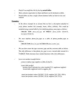
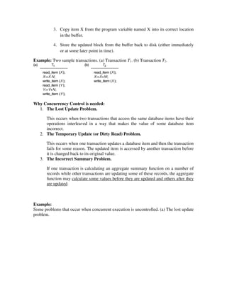
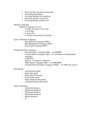
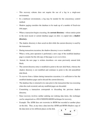
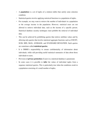
56. - In addition, the log is periodically backed up to archival storage (tape) to guard
against such catastrophic failures.
- T in the following discussion refers to a unique transaction-id that is generated
automatically by the system and is used to identify each transaction:
- Types of log record:
1. [start_transaction,T]: Records that transaction T has started execution.
2. [write_item,T,X,old_value,new_value]: Records that transaction T has
changed the value of database item X from old_value to new_value.
3. [read_item,T,X]: Records that transaction T has read the value of
database item X.
4. [commit,T]: Records that transaction T has completed successfully, and
affirms that its effect can be committed (recorded permanently) to the
database.
5. [abort,T]: Records that transaction T has been aborted.
- Protocols for recovery that avoid cascading rollbacks do not require that read
operations be written to the system log, whereas other protocols require these
entries for recovery.
- Strict protocols require simpler write entries that do not include new_value.
Recovery using log records:
If the system crashes, we can recover to a consistent database state by examining the log
and using one of the recovery techniques.
1. Because the log contains a record of every write operation that changes the value
of some database item, it is possible to undo the effect of these write operations
of a transaction T by tracing backward through the log and resetting all items
changed by a write operation of T to their old_values.
2. We can also redo the effect of the write operations of a transaction T by tracing
forward through the log and setting all items changed by a write operation of T
(that did not get done permanently) to their new_values.
Commit Point of a Transaction:
Definition: A transaction T reaches its commit point when all its operations that access
the database have been executed successfully and the effect of all the transaction
operations on the database has been recorded in the log. Beyond the commit point, the
transaction is said to be committed, and its effect is assumed to be permanently recorded
in the database. The transaction then writes an entry [commit,T] into the log.

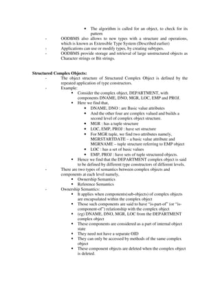
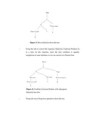
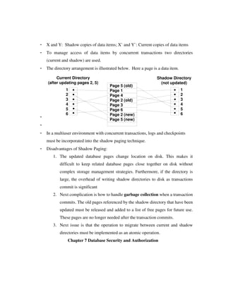
57. Roll Back of transactions: Needed for transactions that have a [start_transaction,T]
entry into the log but no commit entry [commit,T] into the log.
Redoing transactions: Transactions that have written their commit entry in the log must
also have recorded all their write operations in the log; otherwise they would not be
committed, so their effect on the database can be redone from the log entries. (Notice that
the log file must be kept on disk. At the time of a system crash, only the log entries that
have been written back to disk are considered in the recovery process because the
contents of main memory may be lost.)
Force writing a log: before a transaction reaches its commit point, any portion of the
log that has not been written to the disk yet must now be written to the disk. This process
is called force-writing the log file before committing a transaction.
Desirable Properties of Transactions
ACID properties:
- Atomicity: A transaction is an atomic unit of processing; it is either
performed in its entirety or not performed at all.
- Consistency preservation: A correct execution of the transaction must
take the database from one consistent state to another.
- Isolation: A transaction should not make its updates visible to other
transactions until it is committed; this property, when enforced strictly,
solves the temporary update problem and makes cascading rollbacks of
transactions unnecessary.
- Durability or permanency: Once a transaction changes the database and
the changes are committed, these changes must never be lost because of
subsequent failure.
Characterizing Schedules based on Recoverability
- Transaction schedule or history: When transactions are executing
concurrently in an interleaved fashion, the order of execution of operations
from the various transactions forms what is known as a transaction
schedule (or history).
- A schedule (or history) S of n transactions T1, T2, ..., Tn :
- It is an ordering of the operations of the transactions subject to the
constraint that, for each transaction Ti that participates in S, the operations
of T1 in S must appear in the same order in which they occur in T1. Note,
however, that operations from other transactions Tj can be interleaved
with the operations of Ti in S.
Schedules classified on recoverability:
- Recoverable schedule: One where no transaction needs to be rolled back.

58. o A schedule S is recoverable if no transaction T in S commits until all
transactions T’ that have written an item that T reads have committed.
- Cascadeless schedule: One where every transaction reads only the items that are
written by committed transactions.
o Schedules requiring cascaded rollback: A schedule in which
uncommitted transactions that read an item from a failed transaction must
be rolled back.
- Strict Schedules: A schedule in which a transaction can neither read or write an
item X until the last transaction that wrote X has committed.
Characterizing Schedules based on Serializability
- Serial schedule: A schedule S is serial if, for every transaction T participating in
the schedule, all the operations of T are executed consecutively in the schedule.
Otherwise, the schedule is called nonserial schedule.
- Serializable schedule: A schedule S is serializable if it is equivalent to some
serial schedule of the same n transactions.
- Result equivalent: Two schedules are called result equivalent if they produce the
same final state of the database.
- Conflict equivalent: Two schedules are said to be conflict equivalent if the order
of any two conflicting operations is the same in both schedules.
- Conflict serializable: A schedule S is said to be conflict serializable if it is
conflict equivalent to some serial schedule S’.
- Being serializable is not the same as being serial
- Being serializable implies that the schedule is a correct schedule.
- It will leave the database in a consistent state.
- The interleaving is appropriate and will result in a state as if the transactions were
serially executed, yet will achieve efficiency due to concurrent execution.
- Serializability is hard to check.
- Interleaving of operations occurs in an operating system through some scheduler
- Difficult to determine beforehand how the operations in a schedule will be
interleaved.

59. Practical approach:
- Come up with methods (protocols) to ensure serializability.
- It’s not possible to determine when a schedule begins and when it ends. Hence,
we reduce the problem of checking the whole schedule to checking only a
committed project of the schedule (i.e. operations from only the committed
transactions.)
- Current approach used in most DBMSs:
o Use of locks with two phase locking
- View equivalence: A less restrictive definition of equivalence of schedules
- View serializability: definition of serializability based on view equivalence. A
schedule is view serializable if it is view equivalent to a serial schedule.
- Two schedules are said to be view equivalent if the following three conditions
hold:
1. The same set of transactions participates in S and S’, and S and S’ include
the same operations of those transactions.
2. For any operation Ri(X) of Ti in S, if the value of X read by the operation
has been written by an operation Wj(X) of Tj (or if it is the original value
of X before the schedule started), the same condition must hold for the
value of X read by operation Ri(X) of Ti in S’.
3. If the operation Wk(Y) of Tk is the last operation to write item Y in S, then
Wk(Y) of Tk must also be the last operation to write item Y in S’.
The premise behind view equivalence:
- As long as each read operation of a transaction reads the result of the same write
operation in both schedules, the write operations of each transaction musr
produce the same results.
- “The view”: the read operations are said to see the the same view in both
schedules.
Relationship between view and conflict equivalence:
- The two are same under constrained write assumption which assumes that if T
writes X, it is constrained by the value of X it read; i.e., new X = f(old X)

60. - Conflict serializability is stricter than view serializability. With unconstrained
write (or blind write), a schedule that is view serializable is not necessarily
conflict serialiable.
- Any conflict serializable schedule is also view serializable, but not vice versa.
Testing for conflict serializability:
- There is a simple algorithm for determining the conflict serializability of a
schedule.
- Most concurrency control methods do not actually test for serializability.
- Rather protocols, or rules, are developed that guarantee that a schedule will be
serializable.
- We discuss the algorithm for testing conflict serializability of schedules here to
gain a better understanding of these concurrency control protocols
- Algorithm:
1. Looks at only read_Item (X) and write_Item (X) operations
2. Constructs a precedence graph (serialization graph) - a graph with directed
edges
3. An edge is created from Ti to Tj if one of the operations in Ti appears
before a conflicting operation in Tj
4. The schedule is serializable if and only if the precedence graph has no
cycles.
- There are a number of different concurrency control protocols that guarantee
serializability.
o The most common technique, called two-phase locking, is based on
locking data items to prevent concurrent transactions from interfering with
one another, and enforcing an additional condition that guarantees
serializability. This is used in the majority of commercial DBMSs.
o timestamp ordering - where each transaction is assigned a unique
timestamp and the protocol ensures that any conflicting operations are
executed in the order of the transaction timestamps
o multiversion protocol - which are based on maintaining multiple versions
of data items

61. o optimistic (also called certification or validation) protocols, which check
for possible serializability violations after the transactions terminate but
before they are permitted to commit.
Chapter 6 Database Recovery Techniques
Purpose of Database Recovery

62. - To bring the database into the last consistent state, which existed prior to the
failure.
- To preserve transaction properties (Atomicity, Consistency, Isolation and
Durability).
- Example: If the system crashes before a fund transfer transaction completes its
execution, then either one or both accounts may have incorrect value. Thus, the
database must be restored to the state before the transaction modified any of the
accounts.
Types of Failure
- The database may become unavailable for use due to
o Transaction failure: Transactions may fail because of incorrect input,
deadlock, incorrect synchronization.
o System failure: System may fail because of addressing error, application
error, operating system fault, RAM failure, etc.
o Media failure: Disk head crash, power disruption, etc.
Data Update
- Immediate Update: As soon as a data item is modified in cache, the disk copy is
updated.
- Deferred Update: All modified data items in the cache is written either after a
transaction ends its execution or after a fixed number of transactions have
completed their execution.
- Shadow update: The modified version of a data item does not overwrite its disk
copy but is written at a separate disk location.
- In-place update: The disk version of the data item is overwritten by the cache
version.
Data Caching
- Data items to be modified are first stored into database cache by the Cache
Manager (CM) and after modification they are flushed (written) to the disk. The
flushing is controlled by Modified and Pin-Unpin bits.

63. - Pin-Unpin: Instructs the operating system not to flush the data item.
- Modified: Indicates the AFIM of the data item.
Transaction Roll-back (Undo) and Roll-Forward (Redo)
- To maintain atomicity, a transaction’s operations are redone or undone.
- Undo: Restore all BFIMs on to disk (Remove all AFIMs).
- Redo: Restore all AFIMs on to disk.
- Database recovery is achieved either by performing only Undos or only Redos or
by a combination of the two. These operations are recorded in the log as they
happen.
Write-Ahead Logging
- When in-place update (immediate or deferred) is used then log is necessary for
recovery and it must be available to recovery manager. This is achieved by
Write-Ahead Logging (WAL) protocol. WAL states that
- For Undo: Before a data item’s AFIM is flushed to the database disk (overwriting
the BFIM) its BFIM must be written to the log and the log must be saved on a
stable store (log disk).
- For Redo: Before a transaction executes its commit operation, all its AFIMs must
be written to the log and the log must be saved on a stable store.
Checkpointing
- Another type of entry in the log is called a checkpoint
- A [checkpoint] record is written into the log periodically at that point when
the system writes out to the database on disk all DBMS buffers that have been
modified.
- As a consequence of this, all transactions that have their [commit, T] entries in the
log before a [checkpoint] entry do not need to have their WRITE operations
redone in case of a system crash, since all their updates will be recorded in the
database on disk during checkpointing

64. - The recovery manager of a DBMS must decide at what intervals to take a
checkpoint.
- Time to time (randomly or under some criteria) the database flushes its buffer to
database disk to minimize the task of recovery. The following steps defines a
checkpoint operation:
Suspend execution of transactions temporarily.
Force-write modified buffer data to disk.
• Write a [checkpoint] record to the log, save the log to disk.
• Resume normal transaction execution.
- During recovery redo or undo is required to transactions appearing after
[checkpoint] record.
- A checkpoint record in the log may also include additional information, such as a
list of active transaction ids, and the locations (addresses) of the first and most
recent (last) records in the log for each active transaction.
- This can facilitate undoing transaction operations in the event that a transaction
must be rolled back.
- The time needed to force-write all modified memory buffers may delay
transaction processing because of Step 1. To reduce this delay, it is common to
use a technique called fuzzy checkpointing in practice.
In this technique, the system can resume transaction processing
after the [checkpoint] record is written to the log without having to
wait for Step 2 to finish.
However, until Step 2 is completed, the previous [checkpoint]
record should remain to be valid. To accomplish this, the system
maintains
a pointer to the valid checkpoint, which continues to point to the
previous [checkpoint] record in the log.
Once Step 2 is concluded, that pointer is changed to point to the
new checkpoint in the log.

65. Steal/No-Steal and Force/No-Force
Possible ways for flushing database cache to database disk:
- Steal: Cache can be flushed before transaction commits.
- No-Steal: Cache cannot be flushed before transaction commit.
- Force: Cache is immediately flushed (forced) to disk.
- No-Force: Cache is deferred until transaction commits.
These give rise to four different ways for handling recovery:
- Steal/No-Force (Undo/Redo), Steal/Force (Undo/No-redo), No-Steal/No-Force
(Redo/No-undo) and No-Steal/Force (No-undo/No-redo).
Deferred Update
- The idea behind deferred update techniques is to defer or postpone any actual
updates to the database until the transaction completes its execution successfully
and reaches its commit point.
- During transaction execution, the updates are recorded only in the log and in the
cache buffers.
- After the transaction reaches its commit point and the log is force-written to disk,
the updates are recorded in the database.
- If a transaction fails before reaching its commit point, there is no need to undo
any operations, because the transaction has not affected the database on disk in
any way
- Because the database is never updated on disk until after the transaction commits,
there is never a need to UNDO any operations. Hence, this is known as the NO-
UNDO/REDO recovery algorithm.
- REDO is needed in case the system fails after a transaction commits but before all
its changes are recorded in the database on disk. In this case, the transaction
operations are redone from the log entries.
- The data update goes as follows:
•A set of transactions records their updates in the log.

66. •At commit point under WAL scheme these updates are saved on database
disk.
- After reboot from a failure the log is used to redo all the transactions affected by
this failure. No undo is required because no AFIM is flushed to the disk before a
transaction commits.
- A set of transactions records their updates in the log.
- At commit point under WAL scheme these updates are saved on database disk.
- After reboot from a failure the log is used to redo all the transactions affected by
this failure. No undo is required because no AFIM is flushed to the disk before a
transaction commits.
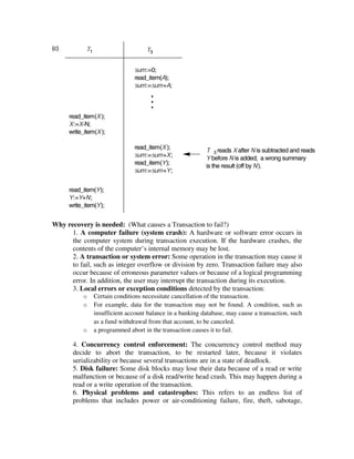
Deferred Update in a single-user system
Example:
(a) T1 T2
read_item (A) read_item (B)
read_item (D) write_item (B)
write_item (D) read_item (D)
write_item (A)
(b)
[start_transaction, T1]
[write_item, T1, D, 20]
[commit T1]
[start_transaction, T1]
[write_item, T2, B, 10]
[write_item, T2, D, 25] ← system crash
- Here the [write_item, …] operations of T1 are redone.
- T2 log entries are ignored by the recovery manager.
- The redo procedure is defined as follows:

67. - REDO(WRITE_OP): Redoing a write_item operation WRITE_OP consists of
examining its log entry [write_item, T, X, new_value] and setting the value of
item X in the database to new_value, which is the after image (AFIM).
- The REDO operation is required to be idempotent—that is, executing it over and
over is equivalent to executing it just once. In fact, the whole recovery process
should be idempotent. This is so because, if the system were to fail during the
recovery process, the next recovery attempt might REDO certain write_item
operations that had already been redone during the first recovery process. The
result of recovery from a system crash during recovery should be the same as the
result of recovering when there is no crash during recovery!
Deferred Update with concurrent users
- This environment requires some concurrency control mechanism to guarantee
isolation property of transactions.
- In a system recovery transactions which were recorded in the log after the last
checkpoint were redone.
- The recovery manager may scan some of the transactions recorded before the
checkpoint to get the AFIMs.
- Two tables are required for implementing this protocol:
- Active table: All active transactions are entered in this table.
- Commit table: Transactions to be committed are entered in this table.
- During recovery, all transactions of the commit table are redone and all
transactions of active tables are ignored since none of their AFIMs reached the
database. It is possible that a commit table transaction may be redone twice but
this does not create any inconsistency because of a redone is “idempotent”, that
is, one redone for an AFIM is equivalent to multiple redone for the same AFIM.
Recovery Techniques Based on Immediate Update

68. - In these techniques, when a transaction issues an update command, the database
can be updated immediately, without any need to wait for the transaction to
reach its commit point.
- In these techniques, however, an update operation must still be recorded in the log
(on disk) before it is applied to the database—using the write-ahead logging
protocol—so that we can recover in case of failure.
- Provisions must be made for undoing the effect of update operations that have
been applied to the database by a failed transaction.
- This is accomplished by rolling back the transaction and undoing the effect of the
transaction’s write_item operations.
- Theoretically, we can distinguish two main categories of immediate update
algorithms.
- If the recovery technique ensures that all updates of a transaction are recorded in
the database on disk before the transaction commits, there is never a need to
REDO any operations of committed transactions.
- This is called the UNDO/NO-REDO recovery algorithm.
- On the other hand, if the transaction is allowed to commit before all its changes
are written to the database, we have the most general case, known as the
UNDO/REDO recovery algorithm.
Undo/No-redo Algorithm
- In this algorithm AFIMs of a transaction are flushed to the database disk under
WAL before it commits.
- For this reason the recovery manager undoes all transactions during recovery.
- No transaction is redone.
- It is possible that a transaction might have completed execution and ready to
commit but this transaction is also undone.
Undo/Redo Algorithm (Single-user environment)

69. - Recovery schemes of this category apply undo and also redo for recovery.
- In a single-user environment no concurrency control is required but a log is
maintained under WAL (Write-Ahead –Logging).
- Note that at any time there will be one transaction in the system and it will be
either in the commit table or in the active table.
- The recovery manager performs:
1. Undo of a transaction if it is in the active table.
2. Redo of a transaction if it is in the commit table.
- The UNDO procedure is defined as follows:
- UNDO(WRITE_OP): Undoing a write_item operation WRITE_OP consists of
examining its log entry [write_item, T, X, old_value, new_value] and setting the
value of item X in the database to old_value which is the before image (BFIM).
Undoing a number of write_item operations from one or more transactions from
the log must proceed in the reverse order from the order in which the operations
were written in the log.
Undo/Redo Algorithm (Concurrent execution)
- Recovery schemes of this category applies undo and also redo to recover the
database from failure.
- In concurrent execution environment a concurrency control is required and log is
maintained under WAL.
- Commit table records transactions to be committed and active table records active
transactions.
- To minimize the work of the recovery manager checkpointing is used. The
recovery performs:
1. Undo of a transaction if it is in the active table.
2. Redo of a transaction if it is in the commit table.
Shadow Paging

70. - This recovery scheme does not require the use of a log in a single-user
environment.
- In a multiuser environment, a log may be needed for the concurrency control
method.
- Shadow paging considers the database to be made up of a number of fixed-size
disk pages.
- When a transaction begins executing, the current directory—whose entries point
to the most recent or current database pages on disk—is copied into a shadow
directory.
- The shadow directory is then saved on disk while the current directory is used by
the transaction.
- During transaction execution, the shadow directory is never modified.
- When a write_item operation is performed, a new copy of the modified database
page is created, but the old copy of that page is not overwritten.
- Instead, the new page is written elsewhere—on some previously unused disk
block.
- The current directory entry is modified to point to the new disk block, whereas the
shadow directory is not modified and continues to point to the old unmodified
disk block.
- To recover from a failure during transaction execution, it is sufficient to free the
modified database pages and to discard the current directory.
- The database thus is returned to its state prior to the transaction that was executing
when the crash occurred, and any modified pages are discarded.
- Committing a transaction corresponds to discarding the previous shadow
directory.
- Since recovery involves neither undoing nor redoing data items, this technique
can be categorized as a NO-UNDO/NO-REDO technique for recovery.
- Example: The AFIM does not overwrite its BFIM but recorded at another place
on the disk. Thus, at any time a data item has AFIM and BFIM (Shadow copy of
the data item) at two different places on the disk.
X Y
Database
X' Y'