Downloaded 15 times
![1
Chapter 1
INTRODUCTION
1.1 INTRODUCTION
Throughout the 1900s, the art of testing without destroying the test object developed from a
laboratory-based experiment to an indispensable tool of fabrication, construction, manufacturing,
and maintenance processes. Nondestructive testing (NDT) comprises methods “to examine a
part, material, or system without impairing its future usefulness” (ASNT 2005). Visual testing has
been replaced by NDT as the primary means of testing the quality of a product. Nondestructive
tests of all sorts are in use worldwide to detect variations in structure, small changes in surface
finish, the presence of cracks or other physical discontinuities, and to measure the thickness of
materials.
Since 1992, the Federal Highway Administration (FHWA) has made available a database
of information on about 600,000 bridges on federal, state, and county roads. The National Bridge
Inventory summarizes the total number of bridges reported by each state. More than a third of
the bridges in the United States were reported as structurally deficient or functionally obsolete in
1992 (USDOT 1996). As of 2004, roughly one in four bridges were considered deficient, with two
out of three not meeting safety standards and nearly one in four recommended for replacement
(USDOT 2004).
The state of the civil infrastructure is a major problem in the United States. Some
problems faced by bridge owners are the detection of deficiencies and the cost of repair,
rehabilitation, and maintenance. Although there exists funding from local, state, and federal
agencies, spending restrictions often keep owners from resolving these issues. Bridge owners
are now using nondestructive testing to assess the condition of bridges. Although visual
inspection has been the main nondestructive tool used in the assessment of these bridges, this
method is inadequate for identification of smaller discontinuities or those hidden or located in
areas that are not easily accessible (ASNT 2005).
Acoustic emission testing is an important method within the broad field of nondestructive
testing. Acoustic emission (AE) is defined by the American Society of Testing Materials (ASTM)
in its Standard Terminology for Nondestructive Evaluations (ASTM E 1316 [2006]) as “the class
of phenomena whereby transient elastic waves are generated by the rapid release of energy from
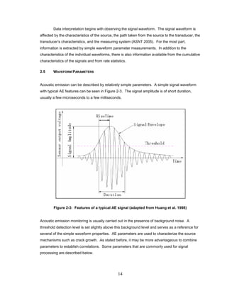
localized sources within a material, or the transient elastic waves so generated.” Acoustic](https://image.slidesharecdn.com/acousticemission-170406030840/85/Acoustic-emission-14-320.jpg)
![13
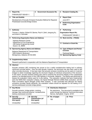
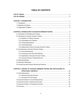
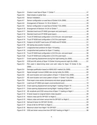
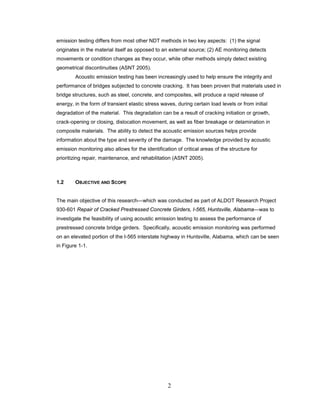
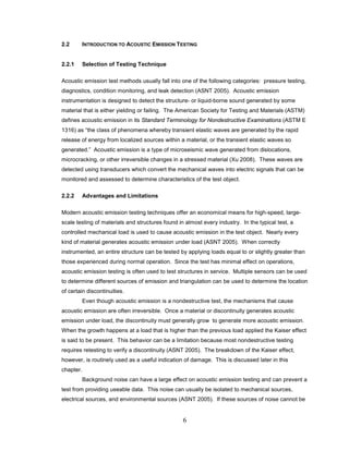
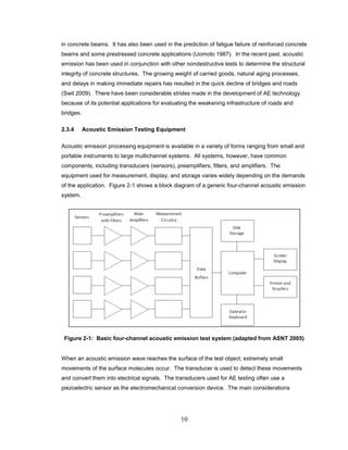
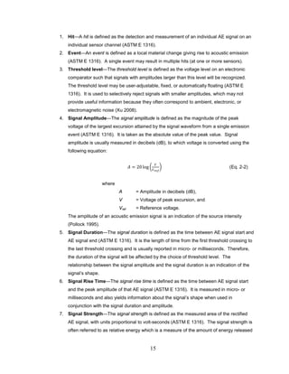
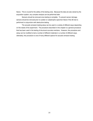
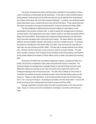
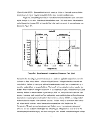
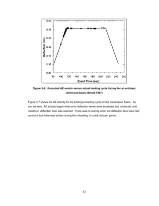
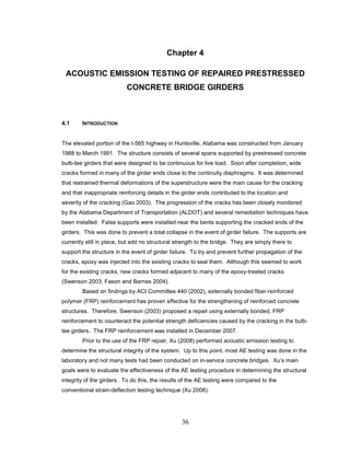
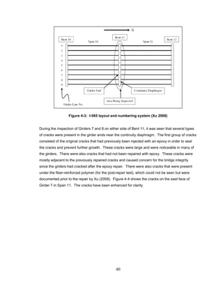
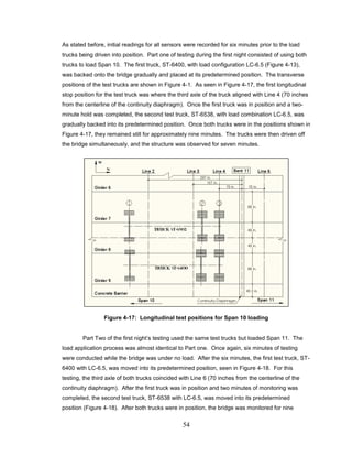
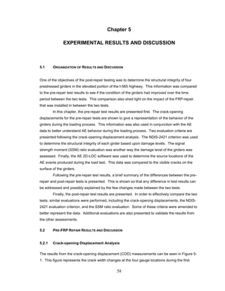
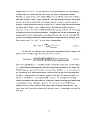
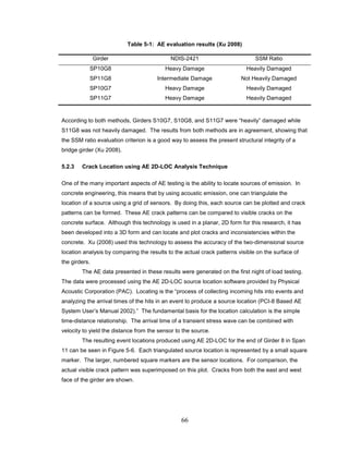
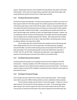
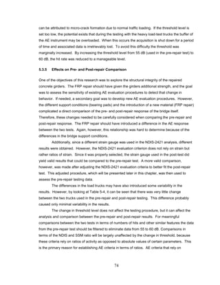
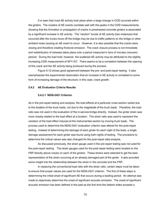
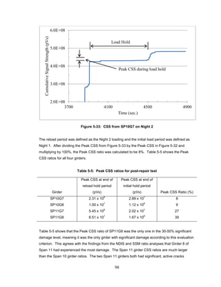
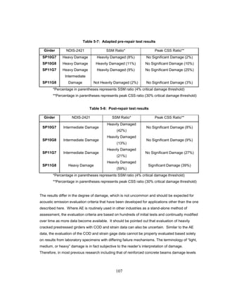
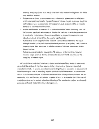
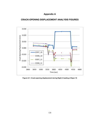
Figure 2-2: Illustration of Kaiser effect and Felicity effect (Adapted from Pollock 1995)
The behavior observed at B (no emission until previous maximum load is exceeded) is
known as the Kaiser effect. Likewise, the behavior at F (emission at load levels less than the
previous maximum) is known as the Felicity effect. According to Pollock (1995), insignificant
flaws tend to exhibit the Kaiser effect, while structurally significant flaws tend to exhibit the Felicity
effect.
According to research, the Kaiser effect fails to occur most noticeably in situations where
time-dependent mechanisms control the deformation (ASNT 2005). Once again, the structure
must be assessed to determine whether the Kaiser effect should be considered for the particular
material and loading process. The Felicity effect can be used in data interpretation depending on
the validity of the Kaiser effect for a certain test.
Another important consideration when dealing with the Kaiser effect is the fact that
friction between free surfaces in damaged regions is a prominent emission mechanism in many
materials. Such source mechanisms contravene the Kaiser effect by emitting waves at low load
levels, but they can still be important for detection of damage and discontinuities (ASNT 2005).
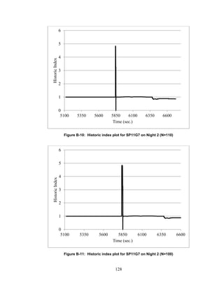
One major complication with interpretation of the Felicity effect is that the “onset of
emission” is not sufficient to establish the effect. Rather, the “onset of significant emission” is
required. The definition of “significant” emission is to some degree subjective and much of the
work related to the Felicity ratio and damage qualifications has been related to quantification of
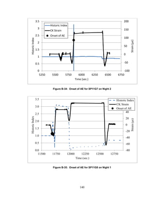
the term “significant.” This has been addressed by some authors through the use of Historic
Index (Ziehl and Fowler 2003), and this approach has been adopted for an ASTM standard test
method related to the design of FRP components (ASTM E 2478 [2006]).
A
C B
DE F
G
Kaiser Effect
Felicity Effect](https://image.slidesharecdn.com/acousticemission-170406030840/85/Acoustic-emission-26-320.jpg)


![104
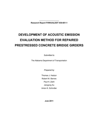
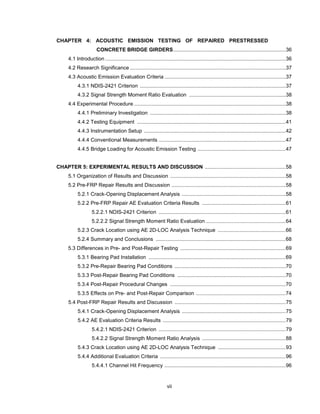
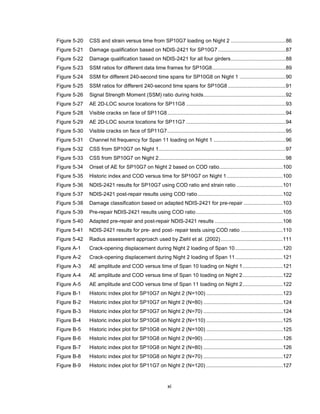
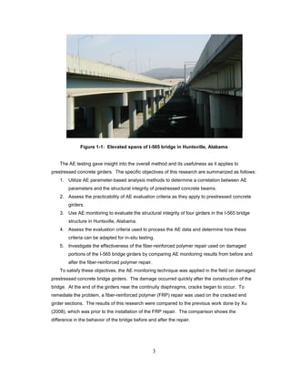
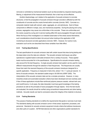
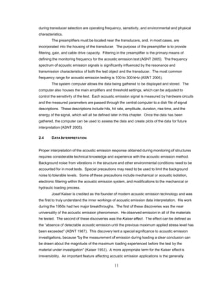
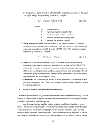
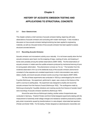
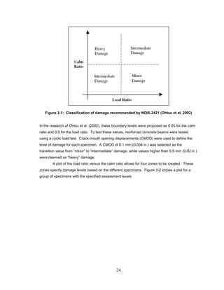
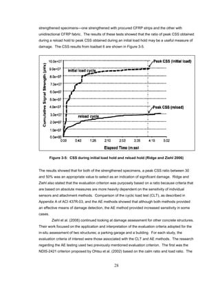
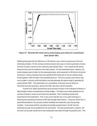
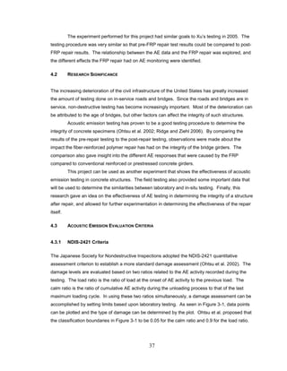
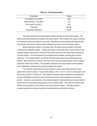
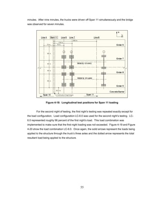
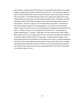
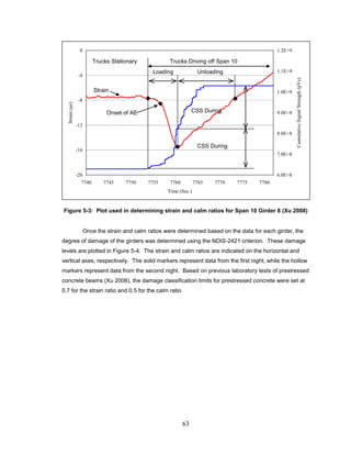
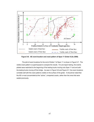
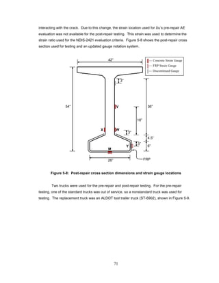
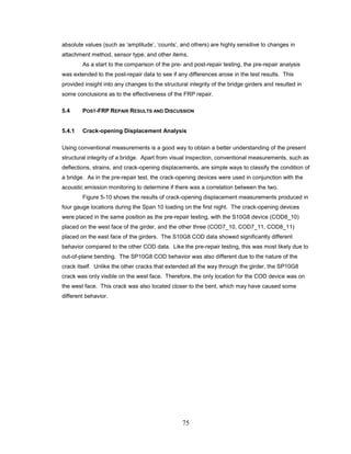
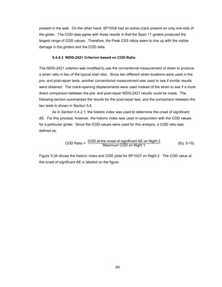
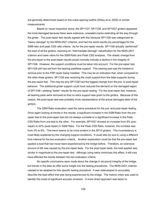
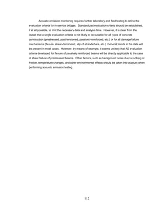
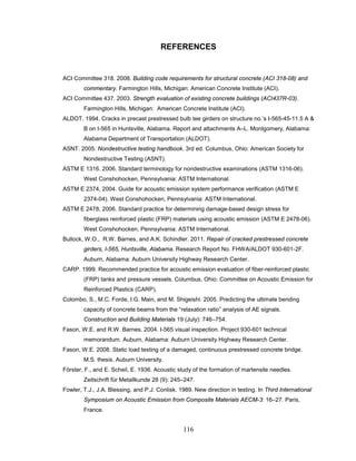
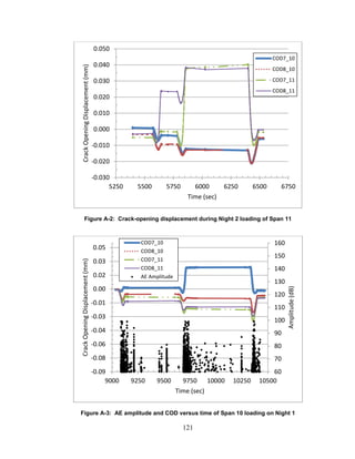
Table 5-6: Peak CSS ratios for pre-repair test
Girder
Peak CSS at end of
reload hold period
(pVs)
Peak CSS at end of
initial hold period
(pVs) Peak CSS Ratio (%)
SP10G7 4.73 x 10
5
2.20 x 10
7
2
SP10G8 5.13 x 10
6
5.32 x 10
7
10
SP11G7 9.34 x 10
6
3.71 x 10
7
25
SP11G8 2.74 x 10
6
9.10 x 10
7
3
As seen in the table, the Peak CSS Ratio analysis indicates that all four of the girders have no
significant damage (based on the 30% critical value proposed by Ridge and Ziehl [2006]). It is
noted that the 30% critical value was developed for reinforced, not prestressed, concrete beams.
This conclusion certainly contradicts the NDIS-2421 results, but some similarities do exist
between the two analyses. First of all, according to the NDIS-2421 criterion, SP11G8 was
classified as “intermediate damage,” while the Peak CSS analysis returned a value of 3%,
signifying very little damage. Likewise, SP11G7 seems to be the most damaged girder of the four
according to the NDIS-2421 criterion, and it yielded the highest Peak CSS ratio.
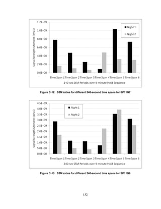
The SSM Ratio analysis used for the post-repair testing was the same analysis used for
the pre-repair analysis, so the results of these two analyses can be compared without adaptation.
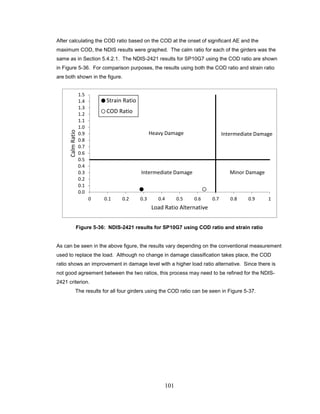
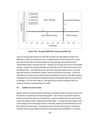
By using the COD ratio for the NDIS-2421 criterion, a direct comparison can be made
between the pre- and post-repair test results. The process described in Section 5.4.4.3 was used
to assess the pre-repair data. The COD ratio NDIS results for the pre-repair test are shown in
Figure 5-39.](https://image.slidesharecdn.com/acousticemission-170406030840/85/Acoustic-emission-117-320.jpg)
![117
Fowler, T.J., L.O. Yepez and C.A. Barnes. 1998. Acoustic emission monitoring of reinforced and
prestressed concrete structures. In Structural Materials Technology III: An NDT
Conference, Proceedings of SPIE 3400: 281–298.
Gao, N. 2003. Investigation of cracking in precast prestressed girders made continuous for live
load. M.S. thesis. Auburn University.
Golaski, L., P. Gebski, and K. Ono. 2002. Diagnostics of reinforced concrete bridges by acoustic
emission. Journal of Acoustic Emission 20: 83–98.
Grosse, C.U. and M. Ohtsu. 2008. Acoustic Emission Testing: Basics for Research—Applications
in Civil Engineering. Berlin: Springer.
Hearn, S.W., and C.K. Shield. 1997. Acoustic emission monitoring as a nondestructive testing
technique in reinforced concrete. ACI Materials Journal 94 (6): 510–519.
Henning, D. 1988. Josef Kaiser: His achievements in AE research. Materials Evaluation 46 (2):
193–195.
Huang, M., L. Jiang, P.K. Liaw, C.R. Brooks, R. Seeley, and D.L. Klarstrom. 1998. Using acoustic
emission in fatigue and fracture materials research. JOM 50 (11).
Kaiser, J. 1950. A study of acoustic phenomena in tensile tests. Dr.-Ing. Dissertation. Technical
University of Munich.
Kishinouye, F. 1932. An experiment on the progression of fracture (a preliminary report). Jishin
6: 25-61. Reprinted in Journal of Acoustic Emission 9 (3): 177–180 [English translation].
Kishinouye, F. 1937. Frequency distribution of the Ito Earthquake Swarm of 1930. Bulletin of the
Earthquake Research Institute (Tokyo Imperial University) 15 (2): 785–826.
L’Hermite, R.G. 1960. Volume changes of concrete. Paper V-3 in Chemistry of Cement:
Proceedings of the 4
th
International Symposium, Washington 1960: 659–694.
Liu, Z. and P.H. Ziehl. 2009. Evaluation of reinforced concrete beam specimens with acoustic
emission and cyclic load test methods. ACI Structural Journal 106 (3): 288–299.
Mason, W.P., J.H. McSkimin, and W. Shockley. 1948. Ultrasonic observation of twinning in tin.
Physical Review 73 (10): 1213–1214.
Millard, D. 1950. Twinning in single crystals of cadmium. Ph.D. thesis. University of Bristol (UK).
Nair, A. 2006. Acoustic emission monitoring and quantitative evaluation of damage in reinforced
concrete members and bridges. M.S. thesis. Louisiana State University.
Niwa, Y., S. Kobayashi, and M. Ohtsu. 1977. Studies of AE in concrete structures. Proceedings
of JSCE 261: 101-112.
Obert, L. 1977. The microseismic method: Discovery and early history. In Proceedings of the
First Conference on Acoustic Emission/Microseismic Activity in Geologic Structures and
Materials. Clausthal, Germany: Trans Tech Publications.](https://image.slidesharecdn.com/acousticemission-170406030840/85/Acoustic-emission-130-320.jpg)

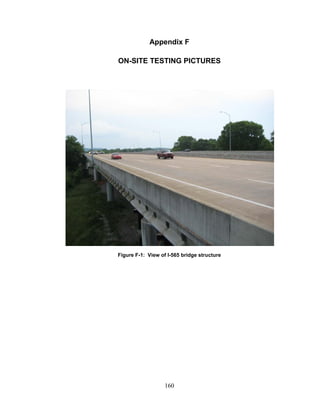

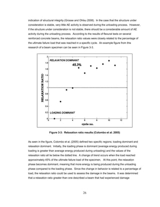
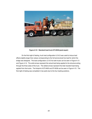
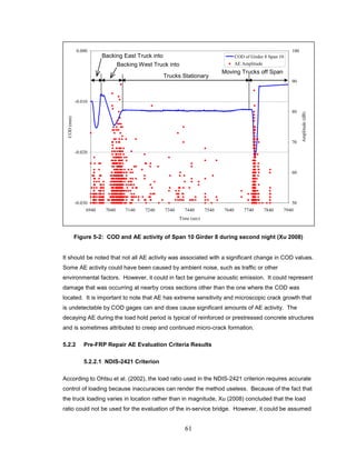
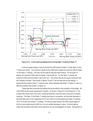
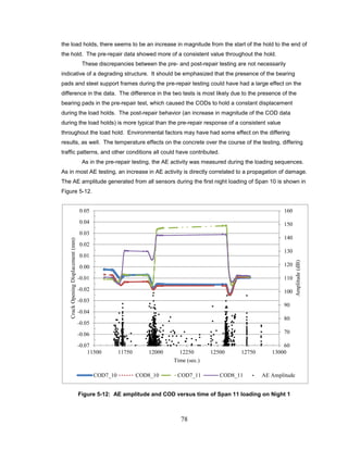
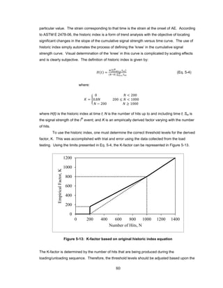
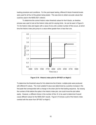
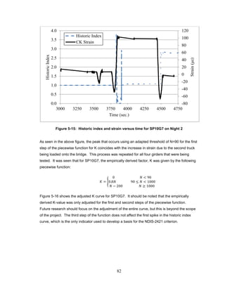
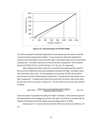
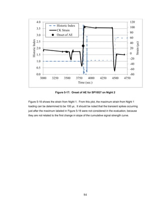
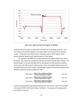
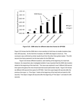
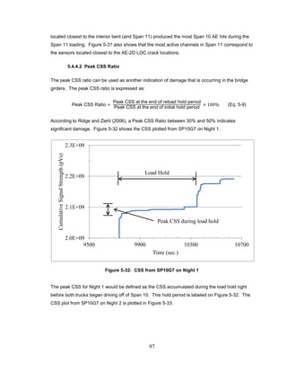
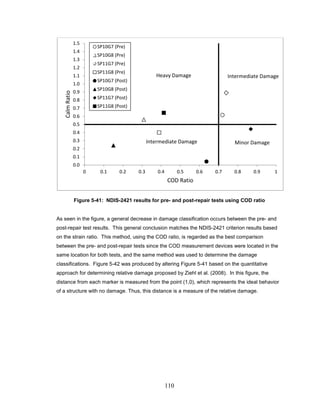
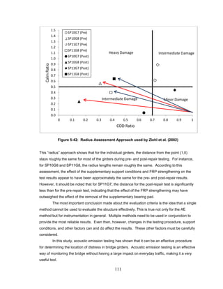
This research report summarizes acoustic emission (AE) testing conducted on four prestressed concrete bridge girders on I-565 in Huntsville, Alabama. The testing was performed to evaluate AE evaluation criteria for assessing the structural integrity of in-service prestressed concrete bridges. Both pre- and post-fiber reinforced polymer (FRP) repair tests were conducted. The evaluation methods used were the NDIS-2421 criterion, signal strength moment ratio analysis, and AE 2D location analysis. It was concluded that while the testing procedure provided results efficiently, the evaluation criteria needed adjustment for testing prestressed concrete bridge girders in service.


