Download to read offline
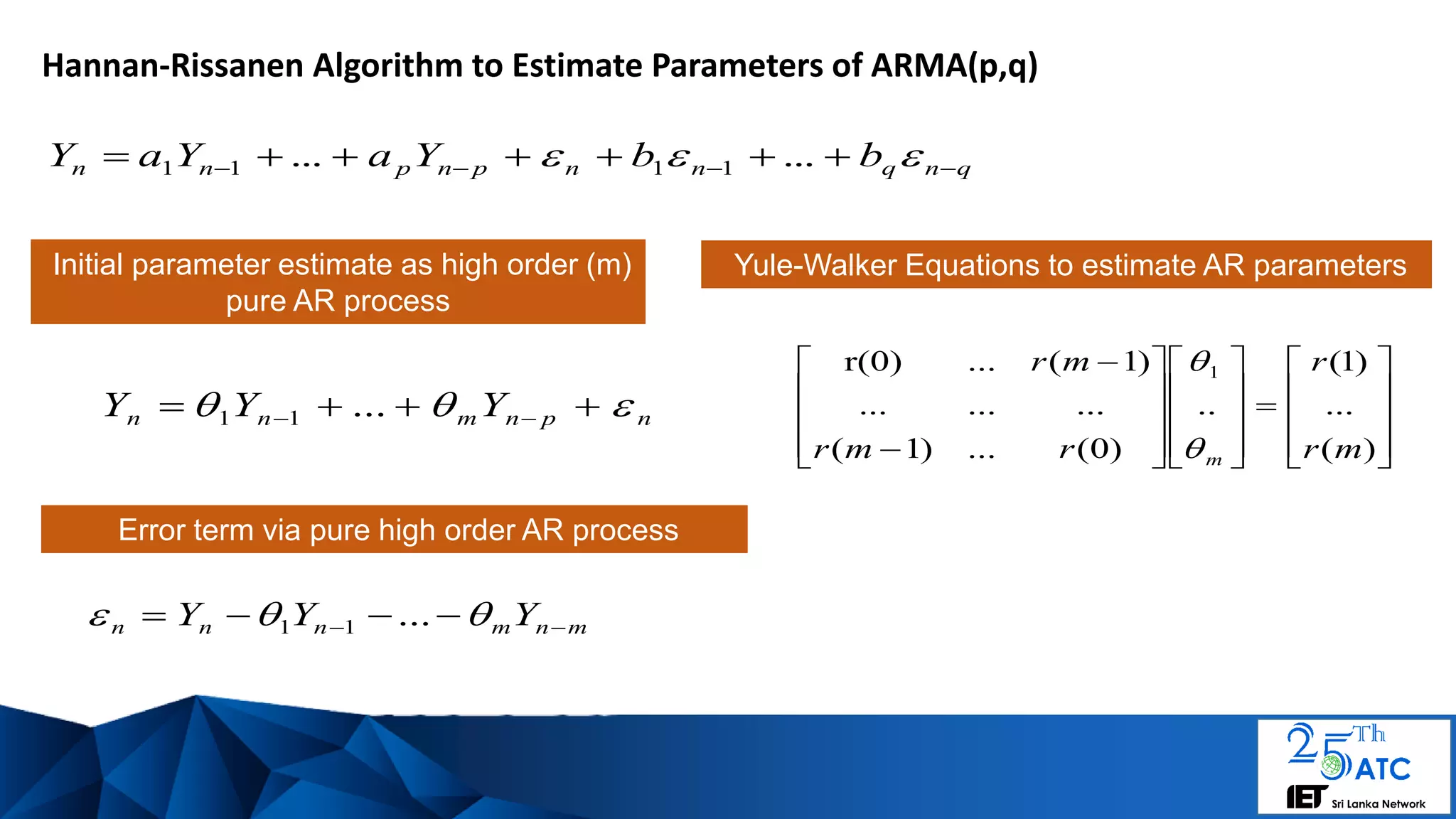
![Hannan-Rissanen Algorithm to Estimate parameters of ARMA(p,q)
Least squares to estimate ARMA parameters
mM
mMMM TT 1
)(
Populate matrix with lagged error terms estimated via pure AR process
nnn YY ˆ
which with some
modifications can
be put in the form
forming a least squares estimate for the ARMA parameters
qnqnpnpnn bbYaYaY ......ˆ
1111where
qpn
pn
pn
n
q
p
qpnqpnqpn
qnnpnn
y
y
y
y
b
b
a
a
y
yy
...
...
...
...
1
...
......
1
1
1
21
1
]...[ 11 qp bbaa](https://image.slidesharecdn.com/modelingpowerconsumptiontimeseriesiet25atc-180820165601/75/A-framework-for-dynamic-pricing-electricity-consumption-patterns-via-time-series-clustering-of-consumer-demand-8-2048.jpg)
![Frequency Response from Pole Zero Map
)(
]...a[1
]...b[1
Y(z) 1
1
1
1
zE
zaz
zbz
p
p
q
q
B(z)
A(z)
n nY
Digital Signal Processing by Proakis and Manolakis
H = Y(z)/E(z) as product of complex roots](https://image.slidesharecdn.com/modelingpowerconsumptiontimeseriesiet25atc-180820165601/75/A-framework-for-dynamic-pricing-electricity-consumption-patterns-via-time-series-clustering-of-consumer-demand-9-2048.jpg)
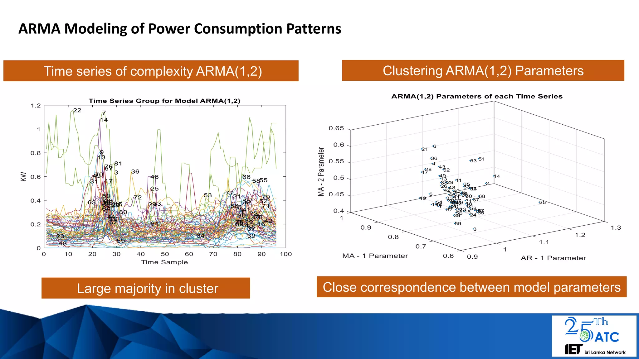
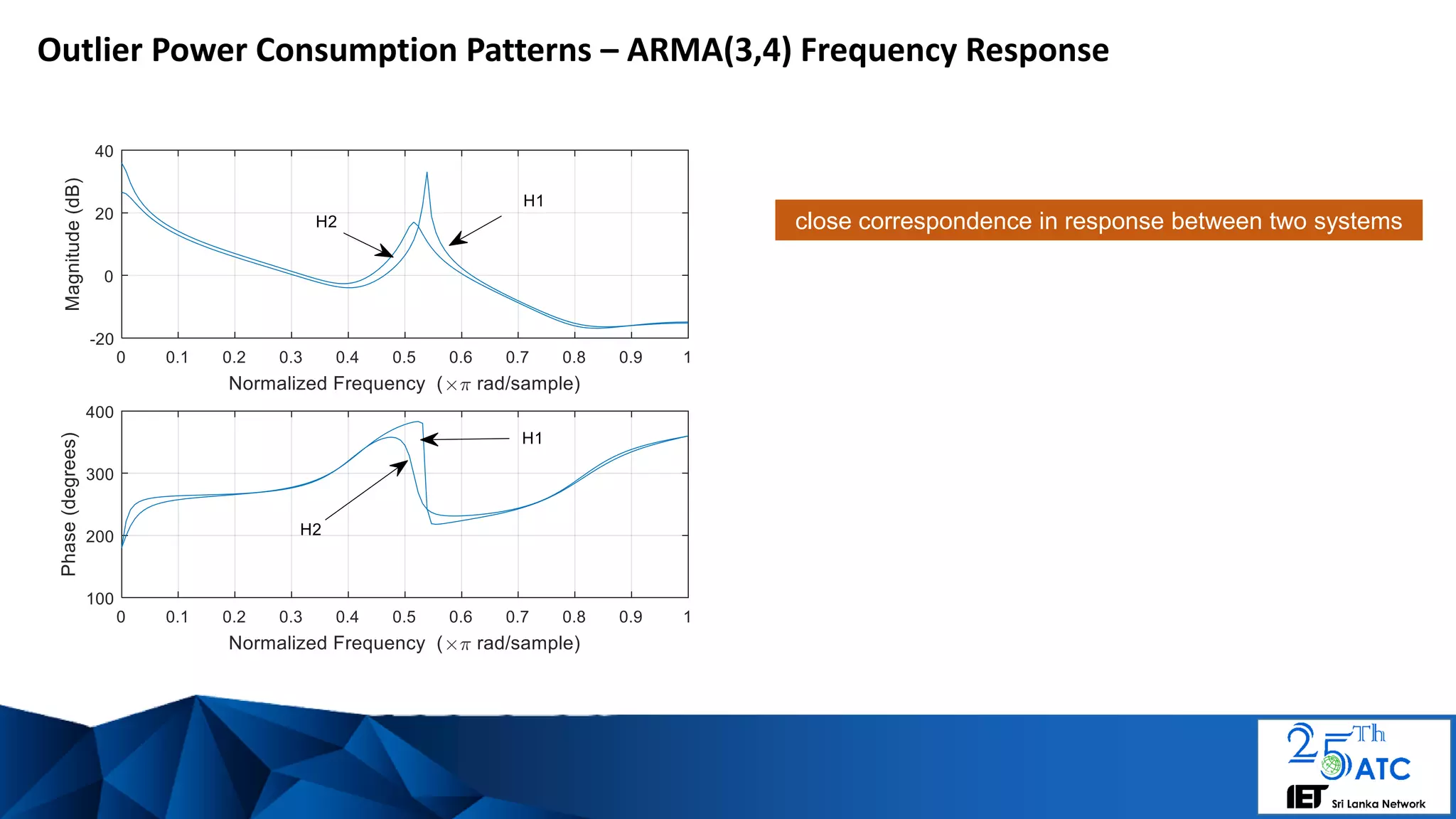
![Outlier Power Consumption Patterns of Complexity ARMA(3,4)
Params: a1 a2 a3 1 b1 b2 b3 b4 ]
[H1 #26: 0.8369 -0.7429 1.0646 1 0.8309 0.6752 0.5491 0.3363]
[H2 #60: 0.9325 -0.8261 0.9477 1 0.8137 0.6589 0.5539 0.3765]
Close match between
ARMA parameters sets](https://image.slidesharecdn.com/modelingpowerconsumptiontimeseriesiet25atc-180820165601/75/A-framework-for-dynamic-pricing-electricity-consumption-patterns-via-time-series-clustering-of-consumer-demand-14-2048.jpg)
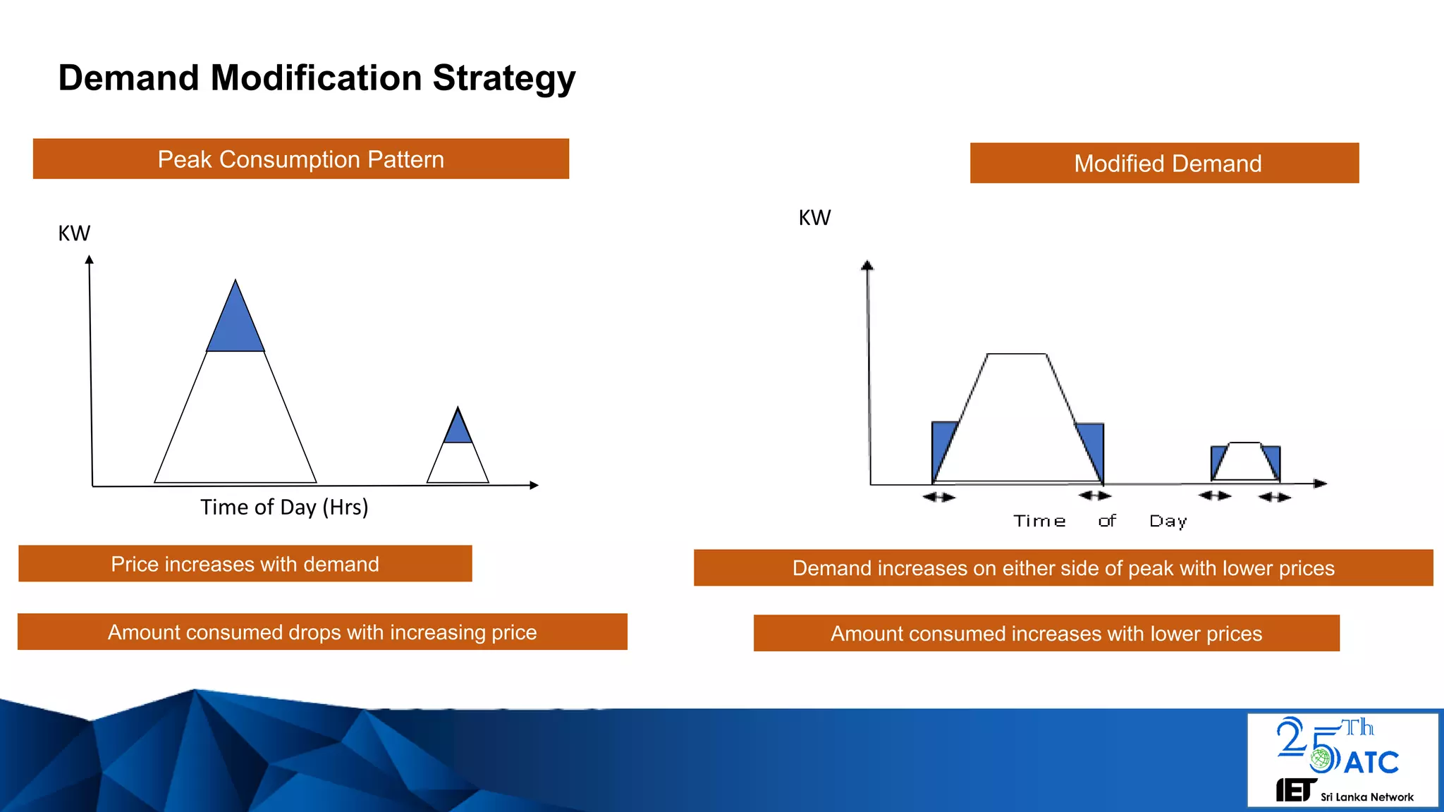

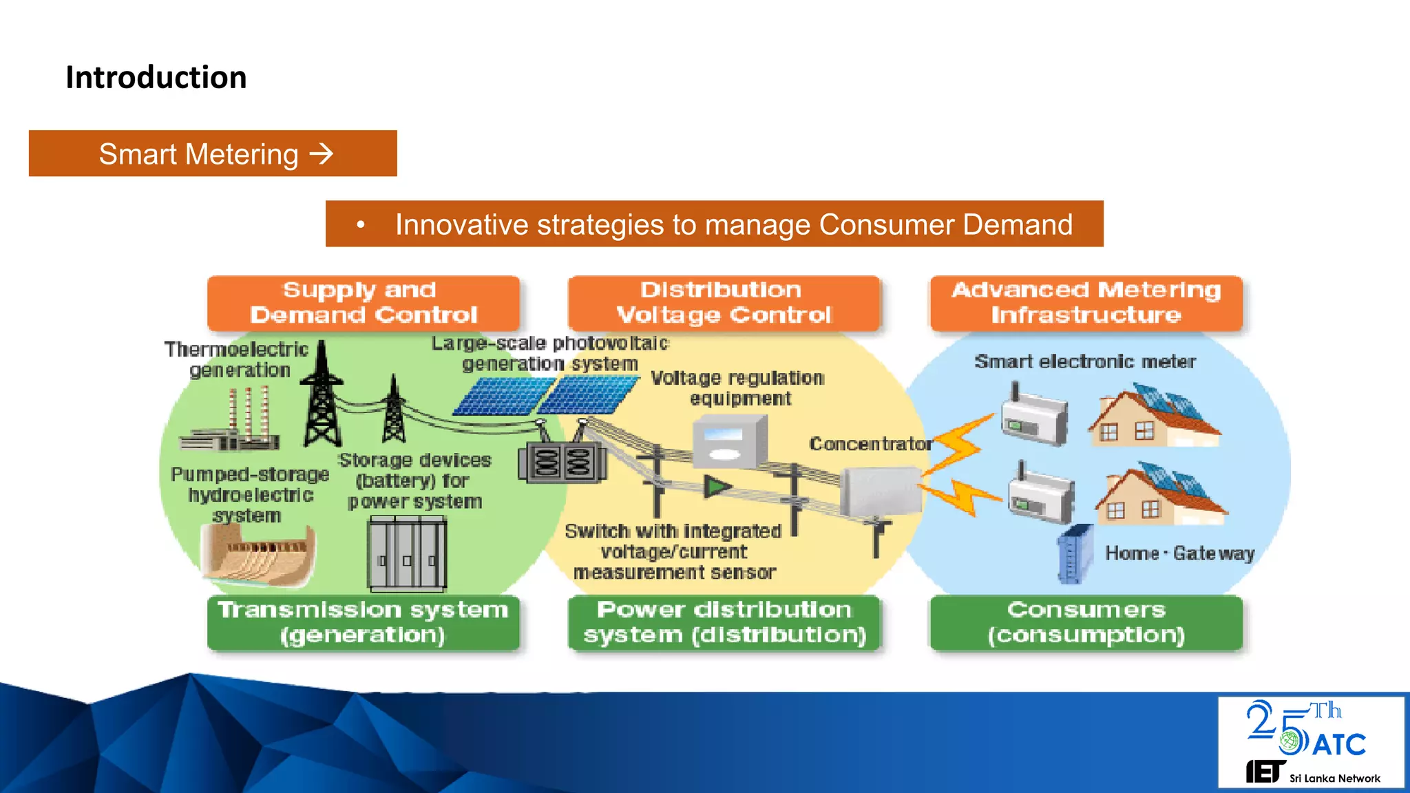
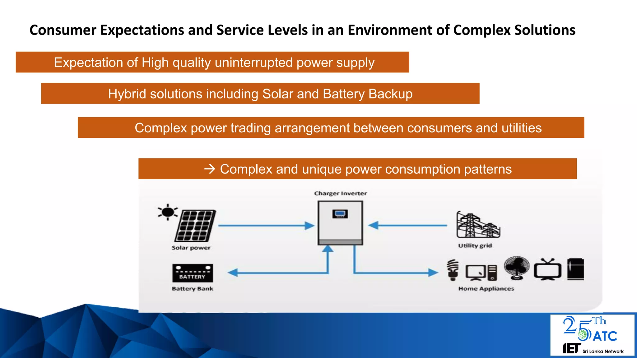
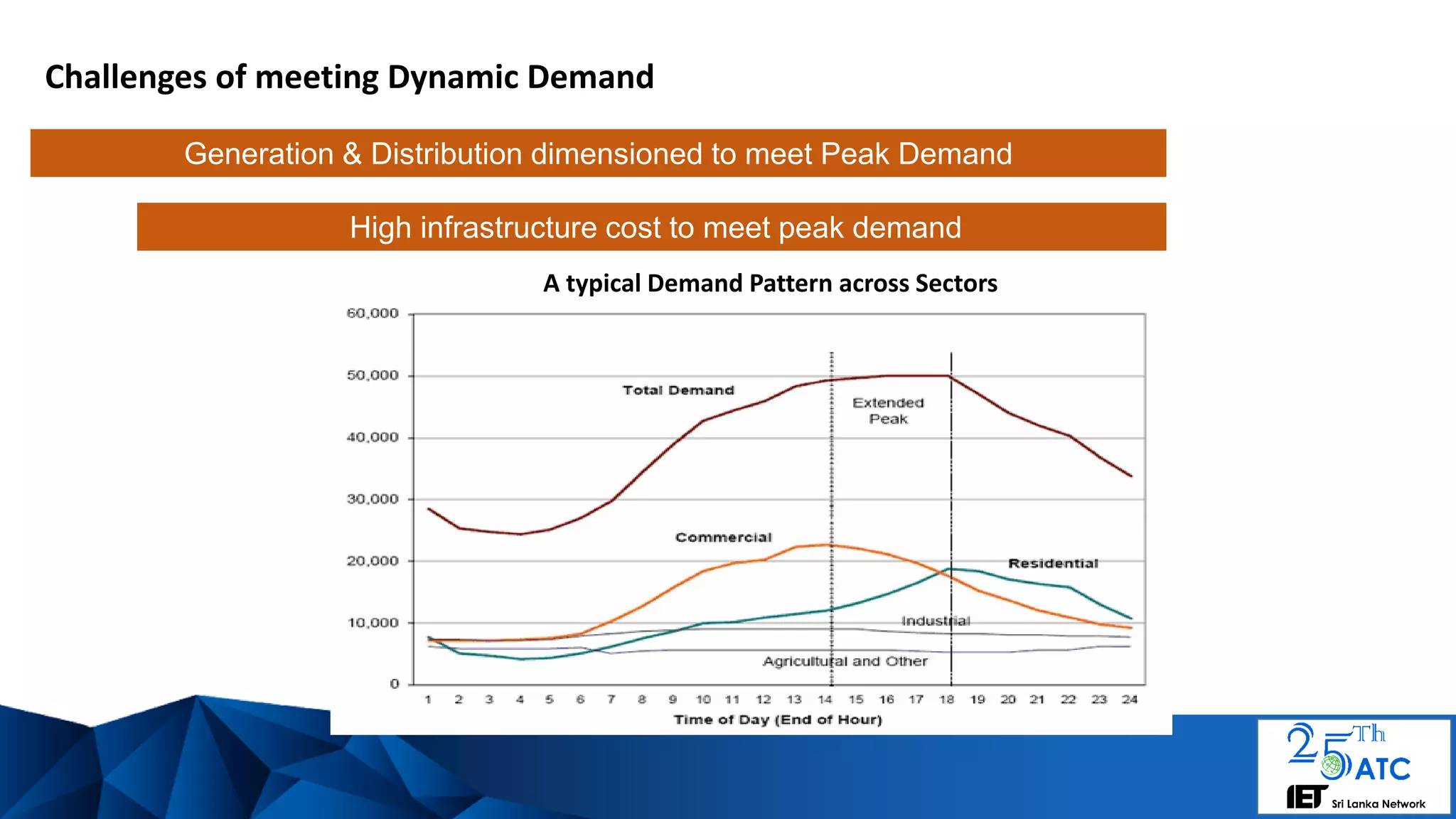
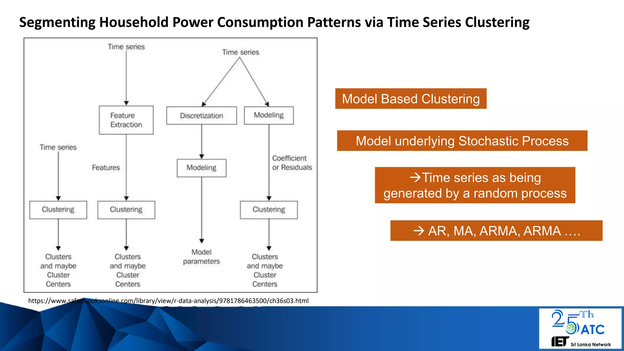
The document discusses a framework for dynamic electricity pricing based on time series clustering of consumer demand patterns to manage consumer expectations and utility supply. It emphasizes the complexities of consumer demand, strategies for segmenting power consumption, and modeling using autoregressive integrated moving average (ARIMA) methods. Additionally, it suggests that unique dynamic pricing strategies can be implemented to address peak demand and identify outlier consumption patterns.