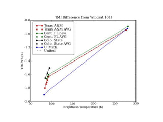
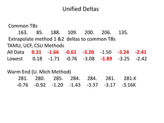
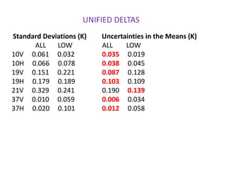
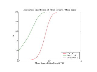
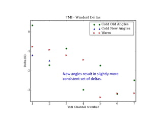
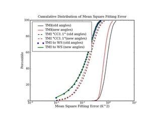
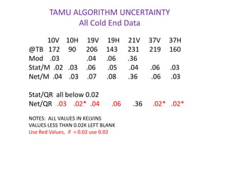
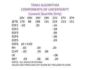
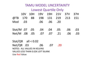
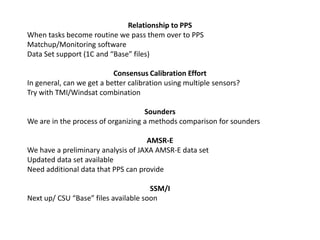
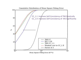
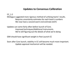
A Consensus Calibration Based on TMI and WindsatTom Wilheit1,Wes Berg2, Linwood Jones3, Rachael Kroodsma4, Darren McKague4, Chris Ruf4, Matt Sapiano2Texas A&M University, (2) Colorado State University, (3) University of Central Florida,  (4) University of Michigan  
GPM Intersatellite Working Group (aka X-CAL)Make Radiances from Constellation Radiometers Physically Consistent	Differences of Frequencies/Incidence AnglesClean Up Other ProblemsVariety of Methods To Generate Two Point Recalibrations	Unified set of DeltasTbnew   = A* Tbold + BCould Be More Complex Where Necessary.Currently Have Consensus Calibration based on Windsat and TMIUse TMI as Transfer Standard. (CC_1.1) (75% Windsat—25% TMI)In Process of Applying to AMSR-E and SSM/I (F13,14,15)Working on CC_1.2    Not Very Different but More Defensible
X-CAL Status OverviewAccuracy:      Relative/ To What Degree can We Make the Sensors Alike?           Looks Like We are Meeting our 0.1K Goal            We Continue to Refine for Sake of Credibility       Absolute             Difficult to Estimate/ Standards are Inadequate              NIST is Working on Standards/ May Impact Satellites in FutureDouble Differences     Where Possible We Use Double Differences to Minimize Model Sensitivity     Corresponding Channels  e.g.    TMI 19.35V/ Windsat 18.7VS = Source Sensor    T= Target SensorDD = (TBTobs – TBTcalc) - (TBSobs – TBScalc)       = (TBTobs – TBSobs) - (TBTcalc– TBScalc)
DATA SETJuly 2005-June 2006TMI Version 7 (Includes reflector temperature correction)WindsatTAMU, UCF, CSU methods use coincident(±1h) observations binned in 1° boxesTAMU solves for SST, WS, PW and CLW using source sensor then computes targetCSU similar to TAMU but external SST and covariancesUCF computes both sets of TBs from GDAS analysesUniv. Michigan cold end method uses global histograms of TBs and finds limiting values.Warm End :  U. Michigan uses method analogous to TAMU and CSU  over Amazon Rain Forest.  JPL and UCF use same method but less mature implementations
Unified Deltas  Common TBs         163.       85.      188.      109.      200.      206.      135. Extrapolate method 1 &2  deltas to common TBsTAMU, UCF, CSU MethodsAll Data      0.31     -1.66     -0.61     -3.20-1.50     -3.24     -2.41Lowest        0.18     -1.71     -0.76     -3.08     -1.89-3.25     -2.42 Warm End (U. Mich Method)         281.      280.       285.      284.      284.       281.       281.K        -0.76     -0.92     -1.20     -1.43     -3.37     -3.17     -3.16K 
UNIFIED DELTASStandard Deviations (K)         Uncertainties in the Means (K)          ALL       LOW	  	ALL        LOW10V     0.061     0.032     	0.035     0.01910H     0.066     0.078     	0.038    0.04519V     0.151     0.221     	0.087     0.12819H     0.179     0.189     	0.103    0.10921V     0.329     0.241     	0.190     0.13937V     0.010     0.059     	0.006     0.03437H     0.020     0.101     	0.012     0.058 
Courtesy of Darren McKague
Consensus CalibrationWarm End Variance   TMI a little more than twice as large as WS (K**2)Cold  End Variance     TMI a little more than three times as large as WSKeep the numbers simple and round        Windsat Gets 3 times the weight of TMI  (i.e. 75%WS/25%TMI)Consensus Calibration 1.175% of Unified DeltasTMI_CC_1.1	10V	10H	19V	19H	21V	37V	37H0.23K	-1.25	-0.46	-2.40	-1.42	-2.43	-1.81     @	163K	85	188	109	200	206	135-0.57K	-0.69	-0.90	-1.07	-2.53	-2.38	2.37      @	281K	280	285	284	284	281	281Negative #’s indicate TMI cold relative to Windsat
Plans for CC_1.2Weights for Unified Deltas based on Error ModelsCommon Partitioning of Cold End Values (Quartiles)Examine Updated Radiative Transfer ModelsEarth Incidence Angle Issue
From Steve Bilanow’s Presentationat March 2011 X-CAL meetingTMI Pointing Uncertainty Effects“Prelaunch measure of TMI 10 V and10H boresight alignment offsets from a 49 degrees scan cone were reported at 0.555 and 0.185 degrees respectively*.                                                                             * Memorandum from Jim Shiue, 12/11/97”This corresponds to ~ 1.3 K and -0.2 K bias shifts.When you do the trigonometry, this translates to increases of the Earth Incidence Angle for the two 10.7 GHz channels  of 0.649° and 0.216°.  (OK, a few too many significant figures)Is it real?Does it matter?
Use   TAMU Model to Calculate  TMI-WS DifferencesWarm End Differences < 0.05K /IgnoreDeltas Computed with TAMU Model	10V 	10H   	19V  	19H 	21V 	37V 	37H	0.34	-1.71	-0.86	-2.98	-1.73	-3.20	-2.49	-1.20	-1.48         Including Jim Shiue’s Angles@	171K	89	202	137	200	216	156	-0.76	-0.92	-1.20	-1.43	-3.37	-3.17	-3.16@	281	280	285	284	284	281	281Deltas are more self-consistent using Jim Shiue’s angles.“TMI_CC_1.1”  based on TAMU model only @ Cold End,  U. Mich  at Warm End.75% Weight for Windsat, 25% TMI
New angles result in slightly more consistent set of deltas.
Conclusions/QuestionsWe have a Consensus Calibration that allows us to move forwardWill be updatedTMI 10 GHz Angle Issue is RealIt Matters (a little)	Needs to be Accounted for Where TMI is being used as a StandardSimilar Problems will recur throughout the ConstellationAccounted for when known Won’t always be Known	Recalibration Will Absorb this Sort of Problem.Goal of X-CAL is 0.1K consistency.	Not all Sensors Will be That Good	Still Not Good Enough For Climate Purposes	Algorithm Team Needs to Think about Another Bias Removal Layer		Average Precipitation in Washington DC  is of order 0.1mm/hAbsolute Accuracy is Another Story	Hesitate to state an error bar
Spare Slides
TAMU ALGORITHMCOMPONENTS OF UNCERTAINTY(All Cold End Data)           10V    10H     19V     19H     21V     37V     37H    @TB   172     90      206     143      231      219     160    EOF1   -.02              .02     -.04       -.26                     EOF2                                    .02        -.09  EOF3                                                   .16EOF4			                    .10EOF5                                                   .05EOF6    all < 0.02RH        .03               .02      .05          .34		        CLHT                         .02      .03LR                                                         .10NET       .03               .04       .06        .36NOTES:  ALL VALUES IN KELVINSVALUES LESS THAN 0.02K LEFT BLANK BUT INCLUDED IN SUMS
TAMU ALGORITHM UNCERTAINTYAll Cold End Data           10V    10H     19V     19H     21V     37V     37H    @TB   172     90      206     143      231      219     160    Mod    .03                .04      .06       .36Stat/M  .02   .03     .06       .05       .04       .06      .03Net/M  .04    .03     .07      .08       .36        .06      .03Stat/QR  all below 0.02Net/QR   .03    .02*  .04       .06       .36      .02*   .02*NOTES:  ALL VALUES IN KELVINSVALUES LESS THAN 0.02K LEFT BLANKUse Red Values,  if  < 0.02 use 0.02
TAMU ALGORITHMCOMPONENTS OF UNCERTAINTY(Lowest Quartile Only)           10V    10H     19V     19H     21V     37V     37H    @TB   170     88      198      131     219      213     151    EOF1   -.02               .02                  -.16                     EOF2                                                 -.04  EOF3                                                  .09EOF4			                  -.06EOF5                                                  .03EOF6    all < 0.02RH          .02               .03                 .20		        CLHT     -.02               .05     .06LR                                                       -.06NET         .03              .06      .06        .20NOTES:  ALL VALUES IN KELVINS/VALUES LESS THAN 0.02K LEFT BLANK BUT INCLUDED IN SUMS
TAMU MODEL UNCERTAINTYLowest Quartile Only       10V    10H     19V     19H     21V     37V     37H    @TB     170     88      198     131     219      213     151    Mod      .03                .06       .06      .20Stat/M  .07    .05       .04      .04      .05        .06      .03Net/M   .08    .05       .07      .07      .21        .06      .03Stat/QR     all < 0.02Net/QR   .03              .06        .07      .20        NOTES:  ALL VALUES IN KELVINSVALUES LESS THAN 0.02K LEFT BLANKUse Red Value
Relationship to PPSWhen tasks become routine we pass them over to PPSMatchup/Monitoring softwareData Set support (1C and “Base” files)Consensus Calibration EffortIn general, can we get a better calibration using multiple sensors?Try with TMI/Windsat combinationSoundersWe are in the process of organizing a methods comparison for soundersAMSR-EWe have a preliminary analysis of JAXA AMSR-E data setUpdated data set availableNeed additional data that PPS can provideSSM/INext up/ CSU “Base” files available soon
CC_1.1  Improves Self-Consistency of TMI DrasticallyCC_1.X  Improves Self-Consistency of  WS Significantly
Updates to Consensus CalibrationCC_1.2McKague suggested more rigorous method of unifying teams’ results.	Requires uncertainty estimates for each team’s numbers	We now have a second warm end estimate (UCF)Updates can come fairly often before launch of Core.	Improved techniques/Additional Instruments	We’re still figuring out the details of what we’re doingGMI should have significant weight in Post Launch CCSoon after Core launch, stability in CC will become much more important.	Update approval mechanism will be needed.
Basics of the TAMU Model3 Reasons to Present:  Collaboration/ Example/Tool Used HereSource Sensor  (e.g. WS)  Surface & AtmosphereTarget (e.g. TMI)Adjust Surface & Atmosphere for best fit to Source RadiancesIterate until Adjustments are < 0.01KFor corresponding channels   DTb is the double difference DTb   = (Tsource – Ttarget)obs   - (Tsource – Ttarget)calcSurface =  Elsaesser Model  (Wilheit/Kohn model has been used for comparison)Modified to allow for negative windspeedsAdjust SST & WSAtmosphere RT Models from RosenkranzModified to allow for Negative Cloud Liquid Water Cloud @ 4-5kmFixed RH Profile/Lapse RateAdjust CLW and Temperature at bottom of Atmosphere (PW follows)
Uncertainties in the TAMU ModelKey Assumptions in the TAMU ModelCloud Location  4 to 5km       Insignificant Contributor to UncertaintyLapse Rate      From Co-located GDAS:   6.26 ± 0.30 K/km      Minor Contribution to UncertaintyRelative Humidity Profile          Mean and Covariance Matrix from Co-located GDAS          Compute EOFs for uncertainty          Primary Source of Uncertainty
A Consensus Calibration Based on TMI and Windsat

A Consensus Calibration Based on TMI and Windsat

  • 1.
    A Consensus CalibrationBased on TMI and WindsatTom Wilheit1,Wes Berg2, Linwood Jones3, Rachael Kroodsma4, Darren McKague4, Chris Ruf4, Matt Sapiano2Texas A&M University, (2) Colorado State University, (3) University of Central Florida, (4) University of Michigan  
  • 2.
    GPM Intersatellite WorkingGroup (aka X-CAL)Make Radiances from Constellation Radiometers Physically Consistent Differences of Frequencies/Incidence AnglesClean Up Other ProblemsVariety of Methods To Generate Two Point Recalibrations Unified set of DeltasTbnew = A* Tbold + BCould Be More Complex Where Necessary.Currently Have Consensus Calibration based on Windsat and TMIUse TMI as Transfer Standard. (CC_1.1) (75% Windsat—25% TMI)In Process of Applying to AMSR-E and SSM/I (F13,14,15)Working on CC_1.2 Not Very Different but More Defensible
  • 3.
    X-CAL Status OverviewAccuracy: Relative/ To What Degree can We Make the Sensors Alike? Looks Like We are Meeting our 0.1K Goal We Continue to Refine for Sake of Credibility Absolute Difficult to Estimate/ Standards are Inadequate NIST is Working on Standards/ May Impact Satellites in FutureDouble Differences Where Possible We Use Double Differences to Minimize Model Sensitivity Corresponding Channels e.g. TMI 19.35V/ Windsat 18.7VS = Source Sensor T= Target SensorDD = (TBTobs – TBTcalc) - (TBSobs – TBScalc) = (TBTobs – TBSobs) - (TBTcalc– TBScalc)
  • 4.
    DATA SETJuly 2005-June2006TMI Version 7 (Includes reflector temperature correction)WindsatTAMU, UCF, CSU methods use coincident(±1h) observations binned in 1° boxesTAMU solves for SST, WS, PW and CLW using source sensor then computes targetCSU similar to TAMU but external SST and covariancesUCF computes both sets of TBs from GDAS analysesUniv. Michigan cold end method uses global histograms of TBs and finds limiting values.Warm End : U. Michigan uses method analogous to TAMU and CSU over Amazon Rain Forest. JPL and UCF use same method but less mature implementations
  • 6.
    Unified Deltas  CommonTBs 163. 85. 188. 109. 200. 206. 135. Extrapolate method 1 &2 deltas to common TBsTAMU, UCF, CSU MethodsAll Data 0.31 -1.66 -0.61 -3.20-1.50 -3.24 -2.41Lowest 0.18 -1.71 -0.76 -3.08 -1.89-3.25 -2.42 Warm End (U. Mich Method) 281. 280. 285. 284. 284. 281. 281.K -0.76 -0.92 -1.20 -1.43 -3.37 -3.17 -3.16K 
  • 7.
    UNIFIED DELTASStandard Deviations(K) Uncertainties in the Means (K) ALL LOW ALL LOW10V 0.061 0.032 0.035 0.01910H 0.066 0.078 0.038 0.04519V 0.151 0.221 0.087 0.12819H 0.179 0.189 0.103 0.10921V 0.329 0.241 0.190 0.13937V 0.010 0.059 0.006 0.03437H 0.020 0.101 0.012 0.058 
  • 9.
  • 10.
    Consensus CalibrationWarm EndVariance TMI a little more than twice as large as WS (K**2)Cold End Variance TMI a little more than three times as large as WSKeep the numbers simple and round Windsat Gets 3 times the weight of TMI (i.e. 75%WS/25%TMI)Consensus Calibration 1.175% of Unified DeltasTMI_CC_1.1 10V 10H 19V 19H 21V 37V 37H0.23K -1.25 -0.46 -2.40 -1.42 -2.43 -1.81 @ 163K 85 188 109 200 206 135-0.57K -0.69 -0.90 -1.07 -2.53 -2.38 2.37 @ 281K 280 285 284 284 281 281Negative #’s indicate TMI cold relative to Windsat
  • 11.
    Plans for CC_1.2Weightsfor Unified Deltas based on Error ModelsCommon Partitioning of Cold End Values (Quartiles)Examine Updated Radiative Transfer ModelsEarth Incidence Angle Issue
  • 12.
    From Steve Bilanow’sPresentationat March 2011 X-CAL meetingTMI Pointing Uncertainty Effects“Prelaunch measure of TMI 10 V and10H boresight alignment offsets from a 49 degrees scan cone were reported at 0.555 and 0.185 degrees respectively*. * Memorandum from Jim Shiue, 12/11/97”This corresponds to ~ 1.3 K and -0.2 K bias shifts.When you do the trigonometry, this translates to increases of the Earth Incidence Angle for the two 10.7 GHz channels of 0.649° and 0.216°. (OK, a few too many significant figures)Is it real?Does it matter?
  • 13.
    Use TAMU Model to Calculate TMI-WS DifferencesWarm End Differences < 0.05K /IgnoreDeltas Computed with TAMU Model 10V 10H 19V 19H 21V 37V 37H 0.34 -1.71 -0.86 -2.98 -1.73 -3.20 -2.49 -1.20 -1.48 Including Jim Shiue’s Angles@ 171K 89 202 137 200 216 156 -0.76 -0.92 -1.20 -1.43 -3.37 -3.17 -3.16@ 281 280 285 284 284 281 281Deltas are more self-consistent using Jim Shiue’s angles.“TMI_CC_1.1” based on TAMU model only @ Cold End, U. Mich at Warm End.75% Weight for Windsat, 25% TMI
  • 14.
    New angles resultin slightly more consistent set of deltas.
  • 16.
    Conclusions/QuestionsWe have aConsensus Calibration that allows us to move forwardWill be updatedTMI 10 GHz Angle Issue is RealIt Matters (a little) Needs to be Accounted for Where TMI is being used as a StandardSimilar Problems will recur throughout the ConstellationAccounted for when known Won’t always be Known Recalibration Will Absorb this Sort of Problem.Goal of X-CAL is 0.1K consistency. Not all Sensors Will be That Good Still Not Good Enough For Climate Purposes Algorithm Team Needs to Think about Another Bias Removal Layer Average Precipitation in Washington DC is of order 0.1mm/hAbsolute Accuracy is Another Story Hesitate to state an error bar
  • 17.
  • 18.
    TAMU ALGORITHMCOMPONENTS OFUNCERTAINTY(All Cold End Data) 10V 10H 19V 19H 21V 37V 37H @TB 172 90 206 143 231 219 160 EOF1 -.02 .02 -.04 -.26 EOF2 .02 -.09 EOF3 .16EOF4 .10EOF5 .05EOF6 all < 0.02RH .03 .02 .05 .34 CLHT .02 .03LR .10NET .03 .04 .06 .36NOTES: ALL VALUES IN KELVINSVALUES LESS THAN 0.02K LEFT BLANK BUT INCLUDED IN SUMS
  • 19.
    TAMU ALGORITHM UNCERTAINTYAllCold End Data 10V 10H 19V 19H 21V 37V 37H @TB 172 90 206 143 231 219 160 Mod .03 .04 .06 .36Stat/M .02 .03 .06 .05 .04 .06 .03Net/M .04 .03 .07 .08 .36 .06 .03Stat/QR all below 0.02Net/QR .03 .02* .04 .06 .36 .02* .02*NOTES: ALL VALUES IN KELVINSVALUES LESS THAN 0.02K LEFT BLANKUse Red Values, if < 0.02 use 0.02
  • 20.
    TAMU ALGORITHMCOMPONENTS OFUNCERTAINTY(Lowest Quartile Only) 10V 10H 19V 19H 21V 37V 37H @TB 170 88 198 131 219 213 151 EOF1 -.02 .02 -.16 EOF2 -.04 EOF3 .09EOF4 -.06EOF5 .03EOF6 all < 0.02RH .02 .03 .20 CLHT -.02 .05 .06LR -.06NET .03 .06 .06 .20NOTES: ALL VALUES IN KELVINS/VALUES LESS THAN 0.02K LEFT BLANK BUT INCLUDED IN SUMS
  • 21.
    TAMU MODEL UNCERTAINTYLowestQuartile Only 10V 10H 19V 19H 21V 37V 37H @TB 170 88 198 131 219 213 151 Mod .03 .06 .06 .20Stat/M .07 .05 .04 .04 .05 .06 .03Net/M .08 .05 .07 .07 .21 .06 .03Stat/QR all < 0.02Net/QR .03 .06 .07 .20 NOTES: ALL VALUES IN KELVINSVALUES LESS THAN 0.02K LEFT BLANKUse Red Value
  • 24.
    Relationship to PPSWhentasks become routine we pass them over to PPSMatchup/Monitoring softwareData Set support (1C and “Base” files)Consensus Calibration EffortIn general, can we get a better calibration using multiple sensors?Try with TMI/Windsat combinationSoundersWe are in the process of organizing a methods comparison for soundersAMSR-EWe have a preliminary analysis of JAXA AMSR-E data setUpdated data set availableNeed additional data that PPS can provideSSM/INext up/ CSU “Base” files available soon
  • 25.
    CC_1.1 ImprovesSelf-Consistency of TMI DrasticallyCC_1.X Improves Self-Consistency of WS Significantly
  • 26.
    Updates to ConsensusCalibrationCC_1.2McKague suggested more rigorous method of unifying teams’ results. Requires uncertainty estimates for each team’s numbers We now have a second warm end estimate (UCF)Updates can come fairly often before launch of Core. Improved techniques/Additional Instruments We’re still figuring out the details of what we’re doingGMI should have significant weight in Post Launch CCSoon after Core launch, stability in CC will become much more important. Update approval mechanism will be needed.
  • 27.
    Basics of theTAMU Model3 Reasons to Present: Collaboration/ Example/Tool Used HereSource Sensor (e.g. WS)  Surface & AtmosphereTarget (e.g. TMI)Adjust Surface & Atmosphere for best fit to Source RadiancesIterate until Adjustments are < 0.01KFor corresponding channels DTb is the double difference DTb = (Tsource – Ttarget)obs - (Tsource – Ttarget)calcSurface = Elsaesser Model (Wilheit/Kohn model has been used for comparison)Modified to allow for negative windspeedsAdjust SST & WSAtmosphere RT Models from RosenkranzModified to allow for Negative Cloud Liquid Water Cloud @ 4-5kmFixed RH Profile/Lapse RateAdjust CLW and Temperature at bottom of Atmosphere (PW follows)
  • 28.
    Uncertainties in theTAMU ModelKey Assumptions in the TAMU ModelCloud Location 4 to 5km Insignificant Contributor to UncertaintyLapse Rate From Co-located GDAS: 6.26 ± 0.30 K/km Minor Contribution to UncertaintyRelative Humidity Profile Mean and Covariance Matrix from Co-located GDAS Compute EOFs for uncertainty Primary Source of Uncertainty