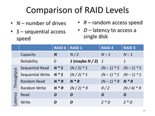
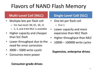
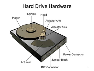
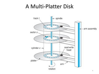
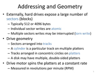
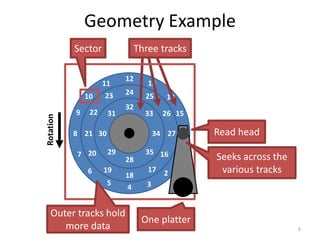
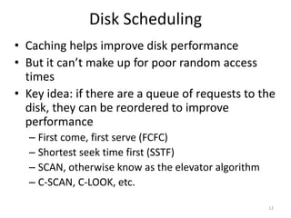
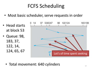
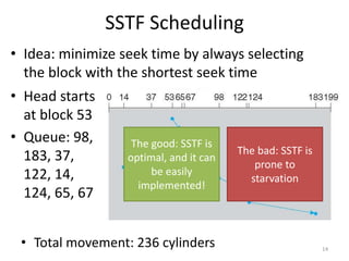
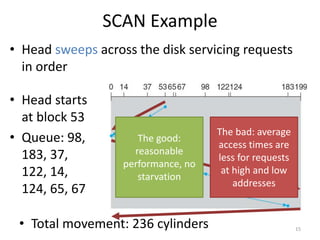
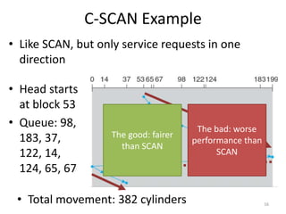
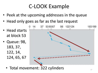
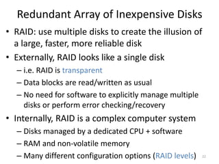
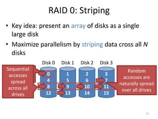
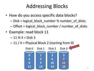
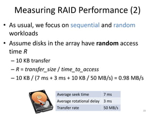
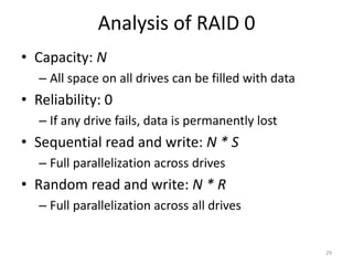
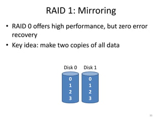
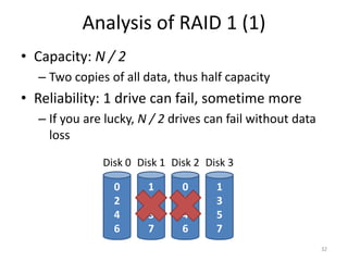
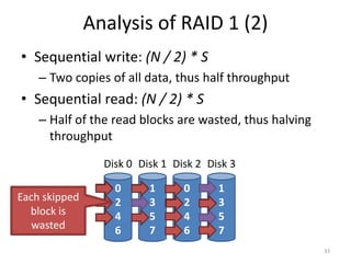
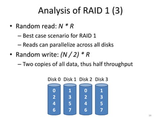
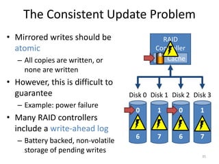
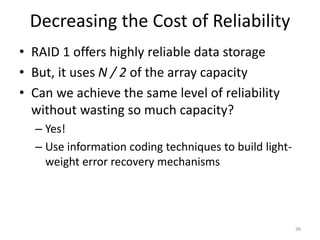
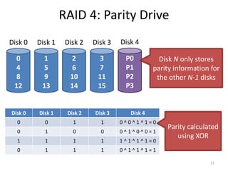
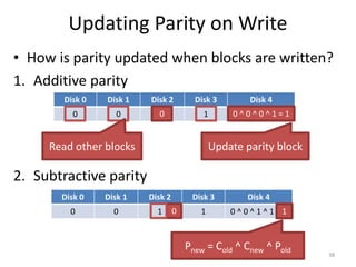
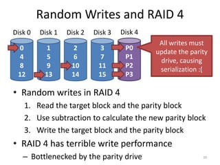
Hard drives store data on spinning platters, with sectors arranged in concentric tracks. RAID arrays distribute data across multiple disks for increased capacity, performance, and reliability. RAID levels 0 and 1 provide different tradeoffs - RAID 0 uses striping for higher performance but no redundancy, while RAID 1 uses mirroring to allow any single disk failure but halves write performance and capacity. Proper scheduling of read/write requests can improve disk performance under different access patterns like sequential versus random.

1. Disk and Drivers

2. • Hard Drives
• RAID
• SSD
2

3. Hard Drive Hardware
3

4. A Multi-Platter Disk
4

5. Addressing and Geometry
• Externally, hard drives expose a large number of
sectors (blocks)
– Typically 512 or 4096 bytes
– Individual sector writes are atomic
– Multiple sectors writes may be interrupted (torn write)
• Drive geometry
– Sectors arranged into tracks
– A cylinder is a particular track on multiple platters
– Tracks arranged in concentric circles on platters
– A disk may have multiple, double-sided platters
• Drive motor spins the platters at a constant rate
– Measured in revolutions per minute (RPM)
5

6. Geometry Example
6
0
1
4
8
12
34
28
32
30
35
29
33
31
27
24
21
18
25
26
17
16
23
22
20
19
13
14
15
2
3
11
10
9
6
5
7
Rotation Three tracks
One platter
Sector
Outer tracks hold
more data
Read head
Seeks across the
various tracks

7. Common Disk Interfaces
• ST-506  ATA  IDE  SATA
– Ancient standard
– Commands (read/write) and addresses in
cylinder/head/sector format placed in device registers
– Recent versions support Logical Block Addresses (LBA)
• SCSI (Small Computer Systems Interface)
– Packet based, like TCP/IP
– Device translates LBA to internal format (e.g. c/h/s)
– Transport independent
• USB drives, CD/DVD/Bluray, Firewire
• iSCSI is SCSI over TCP/IP and Ethernet 7

8. Types of Delay With Disks
8
Three types of delay
1. Rotational Delay
– Time to rotate the desired
sector to the read head
– Related to RPM
2. Seek delay
– Time to move the read
head to a different track
3. Transfer time
– Time to read or write bytes
0
1
4
8
12
34
28
32
30
35
29
33
31
27
24
21
18
25
26
17
16
23
22
20
19
13
14
15
2
3
11
10
9
6
5
7
Short delay
Long delay
Track skew: offset sectors so
that sequential reads across
tracks incorporate seek delay

9. How To Calculate Transfer Time
Cheetah 15K.5 Barracuda
Capacity 300 GB 1 TB
RPM 15000 7200
Avg. Seek 4 ms 9 ms
Max Transfer 125 MB/s 105 MB/s
9
Transfer time
TI/O = Tseek + Trotation + Ttransfer
Assume we are transferring
4096 bytes
TI/O = 4 ms + 1 / (15000 RPM / 60 s/M / 1000 ms/s) / 2
+ (4096 B / 125 MB/s * 1000 ms/s / 220 MB/B)
TI/O = 4 ms + 2ms + 0.03125 ms ≈ 6 ms
Cheetah
Barracuda
TI/O = 9 ms + 1 / (7200 RPM / 60 s/M / 1000 ms/s) / 2
+ (4096 B / 105 MB/s * 1000 ms/s / 220 MB/B)
TI/O = 9 ms + 4.17 ms + 0.0372 ms ≈ 13.2 ms

10. Sequential vs. Random Access
Rate of I/O
RI/O = transfer_size / TI/O
10
Access Type Transfer Size Cheetah 15K.5 Barracuda
Random 4096 B
TI/O 6 ms 13.2 ms
RI/O 0.66 MB/s 0.31 MB/s
Sequential 100 MB
TI/O 800 ms 950 ms
RI/O 125 MB/s 105 MB/s
Max Transfer Rate 125 MB/s 105MB/s
Random I/O results in very
poor disk performance!

11. Caching
• Many disks incorporate caches (track buffer)
– Small amount of RAM (8, 16, or 32 MB)
• Read caching
– Reduces read delays due to seeking and rotation
• Write caching
– Write back cache: drive reports that writes are
complete after they have been cached
• Possibly dangerous feature. Why?
– Write through cache: drive reports that writes are
complete after they have been written to disk
• Today, some disks include flash memory for
persistent caching (hybrid drives)
11

12. Disk Scheduling
• Caching helps improve disk performance
• But it can’t make up for poor random access
times
• Key idea: if there are a queue of requests to the
disk, they can be reordered to improve
performance
– First come, first serve (FCFC)
– Shortest seek time first (SSTF)
– SCAN, otherwise know as the elevator algorithm
– C-SCAN, C-LOOK, etc.
12

13. FCFS Scheduling
• Head starts
at block 53
• Queue: 98,
183, 37,
122, 14,
124, 65, 67
13
• Total movement: 640 cylinders
Lot’s of time spent seeking
• Most basic scheduler, serve requests in order

14. SSTF Scheduling
• Idea: minimize seek time by always selecting
the block with the shortest seek time
14
• Total movement: 236 cylinders
• Head starts
at block 53
• Queue: 98,
183, 37,
122, 14,
124, 65, 67
The good: SSTF is
optimal, and it can
be easily
implemented!
The bad: SSTF is
prone to
starvation

15. SCAN Example
• Head sweeps across the disk servicing requests
in order
15
• Total movement: 236 cylinders
• Head starts
at block 53
• Queue: 98,
183, 37,
122, 14,
124, 65, 67
The good:
reasonable
performance, no
starvation
The bad: average
access times are
less for requests
at high and low
addresses

16. C-SCAN Example
• Like SCAN, but only service requests in one
direction
16
• Total movement: 382 cylinders
• Head starts
at block 53
• Queue: 98,
183, 37,
122, 14,
124, 65, 67
The good: fairer
than SCAN
The bad: worse
performance than
SCAN

17. C-LOOK Example
• Peek at the upcoming addresses in the queue
• Head only goes as far as the last request
17
• Total movement: 322 cylinders
• Head starts
at block 53
• Queue: 98,
183, 37,
122, 14,
124, 65, 67

18. Implementing Disk Scheduling
• We have talked about several scheduling problems
that take place in the kernel
– Process scheduling
– Page swapping
• Where should disk scheduling be implemented?
– OS scheduling
• OS can implement SSTF or LOOK by ordering the queue by LBA
• However, the OS cannot account for rotation delay
– On-disk scheduling
• Disk knows the exact position of the head and platters
• Can implement more advanced schedulers (SPTF)
• But, requires specialized hardware and drivers 18

19. Command Queuing
• Feature where a disk stores of queue of
pending read/write requests
– Called Native Command Queuing (NCQ) in SATA
• Disk may reorder items in the queue to
improve performance
– E.g. batch operations to close sectors/tracks
• Supported by SCSI and modern SATA drives
• Tagged command queuing: allows the host to
place constraints on command re-ordering
19

20. • Hard Drives
• RAID
• SSD
20

21. Beyond Single Disks
• Hard drives are great devices
– Relatively fast, persistent storage
• Shortcomings:
– How to cope with disk failure?
• Mechanical parts break over time
• Sectors may become silently corrupted
– Capacity is limited
• Managing files across multiple physical devices is
cumbersome
• Can we make 10x 1 TB drives look like a 10 TB drive?
21

22. Redundant Array of Inexpensive Disks
• RAID: use multiple disks to create the illusion of
a large, faster, more reliable disk
• Externally, RAID looks like a single disk
– i.e. RAID is transparent
– Data blocks are read/written as usual
– No need for software to explicitly manage multiple
disks or perform error checking/recovery
• Internally, RAID is a complex computer system
– Disks managed by a dedicated CPU + software
– RAM and non-volatile memory
– Many different configuration options (RAID levels) 22

23. Example RAID Controller
23
SATA ports
CPU
RAM
Non-volatile
storage

24. RAID 0: Striping
• Key idea: present an array of disks as a single
large disk
• Maximize parallelism by striping data cross all N
disks
24
0
4
8
12
Disk 0
1
5
9
13
Disk 1
2
6
10
14
Disk 2
3
7
11
15
Disk 3
Stripe
Data block =
512 bytes
Random
accesses are
naturally spread
over all drives
Sequential
accesses
spread
across all
drives

25. Addressing Blocks
• How do you access specific data blocks?
– Disk = logical_block_number % number_of_disks
– Offset = logical_block_number / number_of_disks
• Example: read block 11
– 11 % 4 = Disk 3
– 11 / 4 = Physical Block 2 (starting from 0)
25
0
4
8
12
Disk 0
1
5
9
13
Disk 1
2
6
10
14
Disk 2
3
7
11
15
Disk 3

26. Chunk Sizing
26
0
4
8
12
Disk 0
1
5
9
13
Disk 1
2
6
10
14
Disk 2
3
7
11
15
Disk 3
0
1
8
9
Disk 0
2
3
10
11
Disk 1
4
5
12
13
Disk 2
6
7
14
15
Disk 3
Chunk size = 1 block
Chunk size = 2 block
• Chunk size impacts
array performance
– Smaller chunks 
greater parallelism
– Big chunks 
reduced seek times
• Typical arrays use
64KB chunks

27. Measuring RAID Performance (1)
• As usual, we focus on sequential and random
workloads
• Assume disks in the array have sequential access
time S
– 10 MB transfer
– S = transfer_size / time_to_access
– 10 MB / (7 ms + 3 ms + 10 MB / 50 MB/s) = 47.62 MB/s
27
Average seek time 7 ms
Average rotational delay 3 ms
Transfer rate 50 MB/s

28. Measuring RAID Performance (2)
• As usual, we focus on sequential and random
workloads
• Assume disks in the array have random access
time R
– 10 KB transfer
– R = transfer_size / time_to_access
– 10 KB / (7 ms + 3 ms + 10 KB / 50 MB/s) = 0.98 MB/s
28
Average seek time 7 ms
Average rotational delay 3 ms
Transfer rate 50 MB/s

29. Analysis of RAID 0
• Capacity: N
– All space on all drives can be filled with data
• Reliability: 0
– If any drive fails, data is permanently lost
• Sequential read and write: N * S
– Full parallelization across drives
• Random read and write: N * R
– Full parallelization across all drives
29

30. RAID 1: Mirroring
30
0
1
2
3
Disk 0
0
1
2
3
Disk 1
• RAID 0 offers high performance, but zero error
recovery
• Key idea: make two copies of all data

31. RAID 0+1 and 1+0 Examples
31
0
2
4
6
Disk 0
0
2
4
6
Disk 1
1
3
5
7
Disk 2
1
3
5
7
Disk 3
0
2
4
6
Disk 0
1
3
5
7
Disk 1
0
2
4
6
Disk 2
1
3
5
7
Disk 3
Stripe Stripe
Mirror
Mirror Mirror
Stripe
• Combines striping and mirroring
• Superseded by RAID 4, 5, and 6
0+1 1+0

32. Analysis of RAID 1 (1)
• Capacity: N / 2
– Two copies of all data, thus half capacity
• Reliability: 1 drive can fail, sometime more
– If you are lucky, N / 2 drives can fail without data
loss
32
0
2
4
6
Disk 0
1
3
5
7
Disk 1
0
2
4
6
Disk 2
1
3
5
7
Disk 3

33. Analysis of RAID 1 (2)
• Sequential write: (N / 2) * S
– Two copies of all data, thus half throughput
• Sequential read: (N / 2) * S
– Half of the read blocks are wasted, thus halving
throughput
33
0
2
4
6
Disk 0
1
3
5
7
Disk 1
0
2
4
6
Disk 2
1
3
5
7
Disk 3
Each skipped
block is
wasted

34. Analysis of RAID 1 (3)
• Random read: N * R
– Best case scenario for RAID 1
– Reads can parallelize across all disks
• Random write: (N / 2) * R
– Two copies of all data, thus half throughput
34
0
2
4
6
Disk 0
1
3
5
7
Disk 1
0
2
4
6
Disk 2
1
3
5
7
Disk 3

35. The Consistent Update Problem
• Mirrored writes should be
atomic
– All copies are written, or
none are written
• However, this is difficult to
guarantee
– Example: power failure
• Many RAID controllers
include a write-ahead log
– Battery backed, non-volatile
storage of pending writes
35
0
2
4
6
Disk 0
1
3
5
7
Disk 1
0
2
4
6
Disk 2
1
3
5
7
Disk 3
RAID
Controller
Cache

36. Decreasing the Cost of Reliability
• RAID 1 offers highly reliable data storage
• But, it uses N / 2 of the array capacity
• Can we achieve the same level of reliability
without wasting so much capacity?
– Yes!
– Use information coding techniques to build light-
weight error recovery mechanisms
36

37. RAID 4: Parity Drive
37
0
4
8
12
Disk 0
1
5
9
13
Disk 1
2
6
10
14
Disk 2
3
7
11
15
Disk 3
P0
P1
P2
P3
Disk 4
Disk 0 Disk 1 Disk 2 Disk 3 Disk 4
0 0 1 1 0 ^ 0 ^ 1 ^ 1 = 0
0 1 0 0 0 ^ 1 ^ 0 ^ 0 = 1
1 1 1 1 1 ^ 1 ^ 1 ^ 1 = 0
0 1 1 1 0 ^ 1 ^ 1 ^ 1 = 1
Disk N only stores
parity information for
the other N-1 disks
Parity calculated
using XOR

38. Updating Parity on Write
• How is parity updated when blocks are written?
1. Additive parity
38
2. Subtractive parity
Disk 0 Disk 1 Disk 2 Disk 3 Disk 4
0 0 1 1 0 ^ 0 ^ 1 ^ 1 = 0
0 0 ^ 0 ^ 0 ^ 1 = 1
Read other blocks Update parity block
Disk 0 Disk 1 Disk 2 Disk 3 Disk 4
0 0 1 1 0 ^ 0 ^ 1 ^ 1 = 0
0 1
Pnew = Cold ^ Cnew ^ Pold

39. 0
4
8
12
Disk 0
1
5
9
13
Disk 1
2
6
10
14
Disk 2
3
7
11
15
Disk 3
P0
P1
P2
P3
Disk 4
Random Writes and RAID 4
39
• Random writes in RAID 4
1. Read the target block and the parity block
2. Use subtraction to calculate the new parity block
3. Write the target block and the parity block
• RAID 4 has terrible write performance
– Bottlenecked by the parity drive
All writes must
update the parity
drive, causing
serialization :(

40. Analysis of RAID 4
• Capacity: N – 1
– Space on the parity drive is lost
• Reliability: 1 drive can fail
• Sequential Read and write: (N – 1) * S
– Parallelization across all non-parity blocks
• Random Read: (N – 1) * R
– Reads parallelize over all but the parity drive
• Random Write: R / 2
– Writes serialize due to the parity drive
– Each write requires 1 read and 1 write of the parity
drive, thus R / 2 40

41. RAID 5: Rotating Parity
41
0
5
10
15
Disk 0
1
6
11
P3
Disk 1
2
7
P2
12
Disk 2
3
P1
8
13
Disk 3
P0
4
9
14
Disk 4
Disk 0 Disk 1 Disk 2 Disk 3 Disk 4
0 0 1 1 0 ^ 0 ^ 1 ^ 1 = 0
1 0 0 0 ^ 1 ^ 0 ^ 0 = 1 0
1 1 1 ^ 1 ^ 1 ^ 1 = 0 1 1
1 0 ^ 1 ^ 1 ^ 1 = 1 0 1 1
Parity blocks are
spread over all N
disks

42. Random Writes and RAID 5
• Random writes in RAID 5
1. Read the target block and the parity block
2. Use subtraction to calculate the new parity block
3. Write the target block and the parity block
• Thus, 4 total operations (2 reads, 2 writes)
– Distributed across all drives 42
0
5
10
15
Disk 0
1
6
11
P3
Disk 1
2
7
P2
12
Disk 2
3
P1
8
13
Disk 3
P0
4
9
14
Disk 4
Unlike RAID 4,
writes are spread
roughly evenly
across all drives

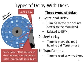
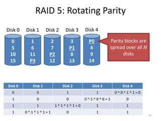
43. Analysis of Raid 5
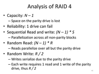
• Capacity: N – 1 [same as RAID 4]
• Reliability: 1 drive can fail [same as RAID 4]
• Sequential Read and write: (N – 1) * S [same]
– Parallelization across all non-parity blocks
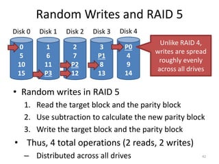
• Random Read: N * R [vs. (N – 1) * R]
– Unlike RAID 4, reads parallelize over all drives
• Random Write: N / 4 * R [vs. R / 2 for RAID 4]
– Unlike RAID 4, writes parallelize over all drives
– Each write requires 2 reads and 2 write, hence N / 4
43

44. Comparison of RAID Levels
RAID 0 RAID 1 RAID 4 RAID 5
Capacity N N / 2 N – 1 N – 1
Reliability 0 1 (maybe N / 2) 1 1
Throughput
Sequential Read N * S (N / 2) * S (N – 1) * S (N – 1) * S
Sequential Write N * S (N / 2) * S (N – 1) * S (N – 1) * S
Random Read N * R N * R (N – 1) * R N * R
Random Write N * R (N / 2) * R R / 2 (N / 4) * R
Latency
Read D D D D
Write D D 2 * D 2 * D
44
• N – number of drives
• S – sequential access
speed
• R – random access speed
• D – latency to access a
single disk

45. RAID 6
• Any two drives can fail
• N – 2 usable capacity
• No overhead on read, significant overhead on write
• Typically implemented using Reed-Solomon codes
45
0
4
8
P30
Disk 0
1
5
P20
P31
Disk 1
2
P10
P21
9
Disk 2
P00
P11
6
10
Disk 3
P01
3
7
11
Disk 4
Two parity blocks
per stripe

46. Choosing a RAID Level
• Best performance and most capacity?
– RAID 0
• Greatest error recovery?
– RAID 1 (1+0 or 0+1) or RAID 6
• Balance between space, performance, and
recoverability?
– RAID 5
46

47. Other Considerations
• Many RAID systems include a hot spare
– An idle, unused disk installed in the system
– If a drive fails, the array is immediately rebuilt using
the hot spare
• RAID can be implemented in hardware or software
– Hardware is faster and more reliable…
– But, migrating a hardware RAID array to a different
hardware controller almost never works
– Software arrays are simpler to migrate and cheaper,
but have worse performance and weaker reliability
• Due to the consistent update problem
47

48. • Hard Drives
• RAID
• SSD
48

49. Beyond Spinning Disks
• Hard drives have been around since 1956
– The cheapest way to store large amounts of data
– Sizes are still increasing rapidly
• However, hard drives are typically the slowest
component in most computers
– CPU and RAM operate at GHz
– PCI-X and Ethernet are GB/s
• Hard drives are not suitable for mobile devices
– Fragile mechanical components can break
– The disk motor is extremely power hungry
49

50. Solid State Drives
• NAND flash memory-based drives
– High voltage is able to change the configuration of
a floating-gate transistor
– State of the transistor interpreted as binary data
50
Flash memory
chip
Data is striped
across all chips

51. Advantages of SSDs
• More resilient against physical damage
– No sensitive read head or moving parts
– Immune to changes in temperature
• Greatly reduced power consumption
– No mechanical, moving parts
• Much faster than hard drives
– >500 MB/s vs ~200 MB/s for hard drives
– No penalty for random access
• Each flash cell can be addressed directly
• No need to rotate or seek
– Extremely high throughput
• Although each flash chip is slow, they are RAIDed 51

52. 52

53. Challenges with Flash
• Flash memory is written in pages, but erased
in blocks
– Pages: 4 – 16 KB, Blocks: 128 – 256 KB
– Thus, flash memory can become fragmented
– Leads to the write amplification problem
• Flash memory can only be written a fixed
number of times
– Typically 3000 – 5000 cycles for MLC
– SSDs use wear leveling to evenly distribute writes
across all flash cells
53

54. Write Amplification
• Once all pages have been written, valid pages
must be consolidated to free up space
• Write amplification: a write triggers garbage
collection/compaction
– One or more blocks must be read, erased, and
rewritten before the write can proceed 54
Block X Block Y
A
B
C
D
E
F
G
A’
B’
C’
D’
E’
F’
D’’
E’’
F’’
H
I
J
A’’’
B’’’
A’’
B’’
C’’
Stale pages
cannot be
overwritten
or erased
individually
G
K
L
G moved to new block
by the garbage collector
Cleaned
block can
now be
rewritten

55. Garbage Collection
• Garbage collection (GC) is vital for the
performance of SSDs
• Older SSDs had fast writes up until all pages
were written once
– Even if the drive has lots of “free space,” each
write is amplified, thus reducing performance
• Many SSDs over-provision to help the GC
– 240 GB SSDs actually have 256 GB of memory
• Modern SSDs implement background GC
– However, this doesn’t always work correctly
55

56. The Ambiguity of Delete
• Goal: the SSD wants to perform background GC
– But this assumes the SSD knows which pages are
invalid
• Problem: most file systems don’t actually delete
data
– On Linux, the “delete” function is unlink()
– Removes the file meta-data, but not the file itself
56

57. Delete Example
1. File is written to SSD
2. File is deleted
3. The GC executes
– 9 pages look valid to the SSD
– The OS knows only 2 pages
are valid
57
Block X
Meta
Meta
File
File
File
File
File
File
File
Meta
Meta
File metadata
(inode, name,
etc.)
Metadata is
overwritten,
but the file
remains
• Lack of explicit delete
means the GC wastes
effort copying useless
pages
• Hard drives are not
GCed, so this was
never a problem

58. TRIM
• New SATA command TRIM (SCSI – UNMAP)
– Allows the OS to tell the SSD that specific LBAs are
invalid, may be GCed
58
• OS support for TRIM
– Win 7, OSX Snow Leopard, Linux 2.6.33, Android 4.3
• Must be supported by the SSD firmware
Block X
Meta
Meta
File
File
File
File
File
File
File
Meta
Meta
TRIM

59. Wear Leveling
• Recall: each flash cell wears out after several
thousand writes
• SSDs use wear leveling to spread writes across
all cells
– Typical consumer SSDs should last ~5 years
59

60. Wear Leveling Examples
60
Block X Block Y
A
B
C
D
E
F
G
A’
B’
C’
D’
E’
F’
D’’
E’’
F’’
H
I
G’
A’’’
B’’’
A’’
B’’
C’’
K
L
Wait as long
as possible
before
garbage
collecting
Block X Block Y
A
B
C
D
E
F
G
H
I
J
K
L
M
N
O
M’
N’
O’
M’’
N’’
O’’
M’’’
N’’’
O’’’
M*
N*
O*
A
B
C
D
E
F
G
H
I
J
K
L
M*
N*
SSD controller periodically swap long
lived data to different blocks
Blocks with
long lived
data receive
less wear
If the GC runs now, page
G must be copied
O*
Dynamic
Wear
Leveling
Static
Wear
Leveling

61. SSD Controllers
• All operations handled by the SSD controller
– Maps LBAs to physical pages
– Keeps track of free pages, controls the GC
– May implement background GC
– Performs wear leveling via data rotation
• Controller performance is crucial for overall
SSD performance
61
• SSDs are extremely complicated
internally

62. Flavors of NAND Flash Memory
Multi-Level Cell (MLC)
• One bit per flash cell
– 0 or 1
• Lower capacity and more
expensive than MLC flash
• Higher throughput than MLC
• 10000 – 100000 write cycles
Expensive, enterprise drives
Single-Level Cell (SLC)
• Multiple bits per flash cell
– For two-level: 00, 01, 10, 11
– 2, 3, and 4-bit MLC is available
• Higher capacity and cheaper
than SLC flash
• Lower throughput due to the
need for error correction
• 3000 – 5000 write cycels
• Consumes more power
Consumer-grade drives
62