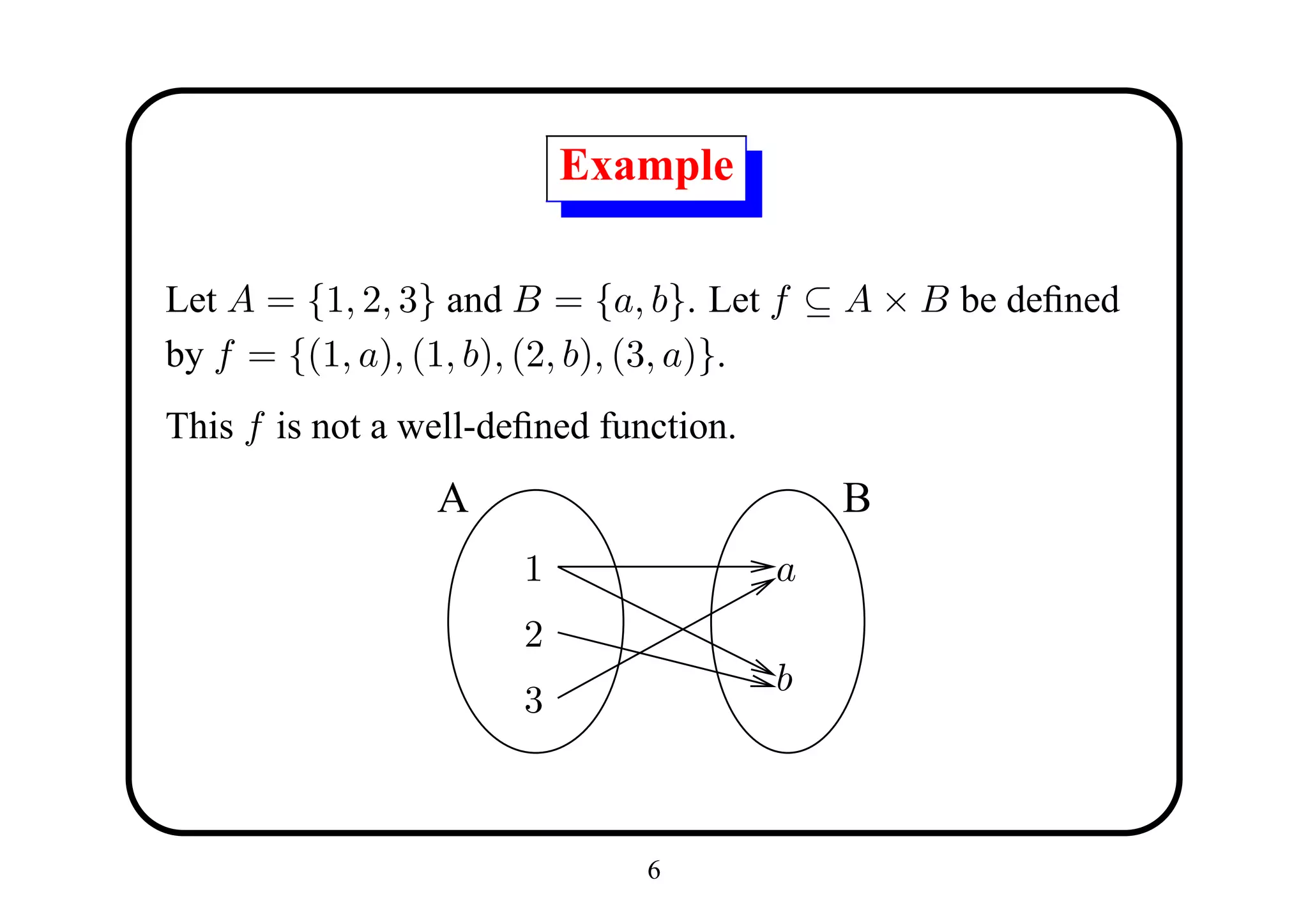
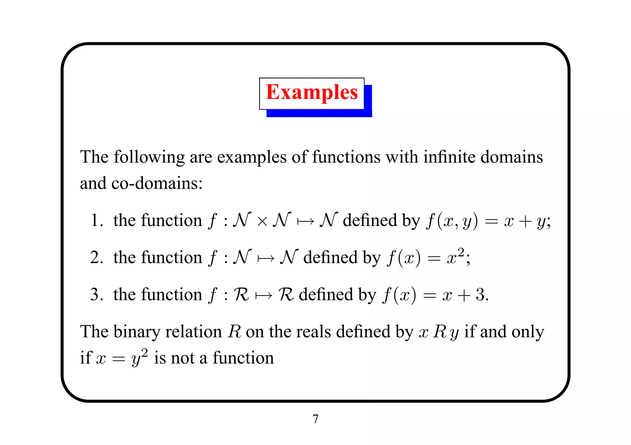
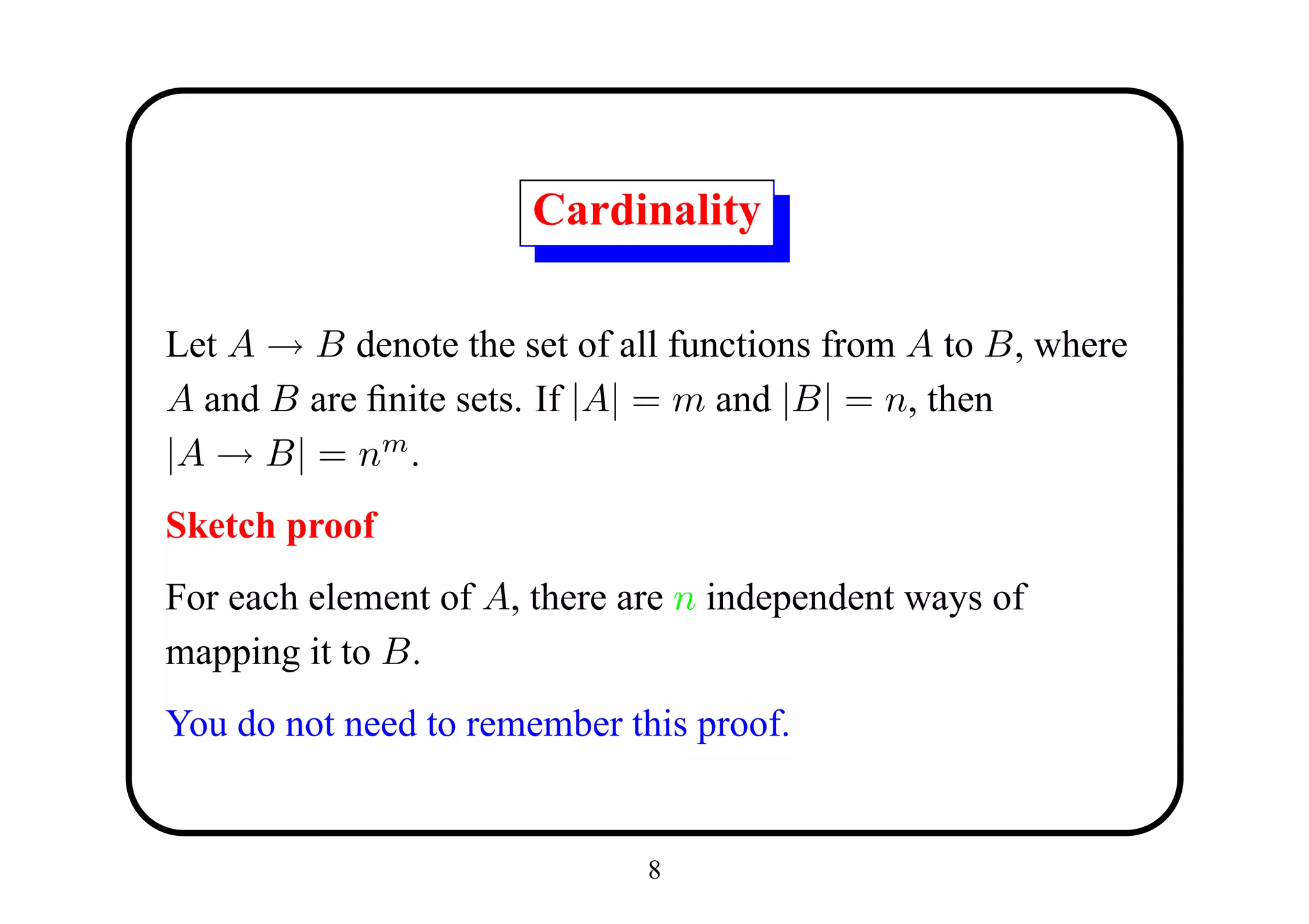
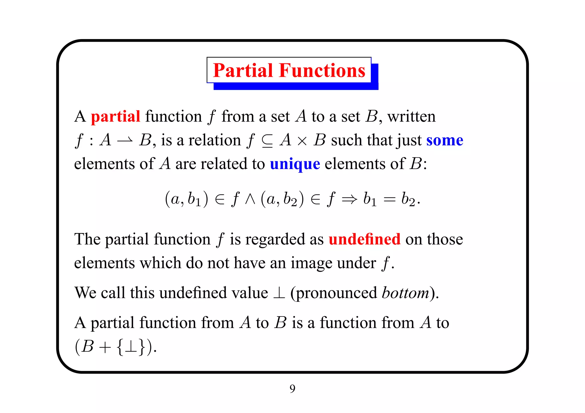
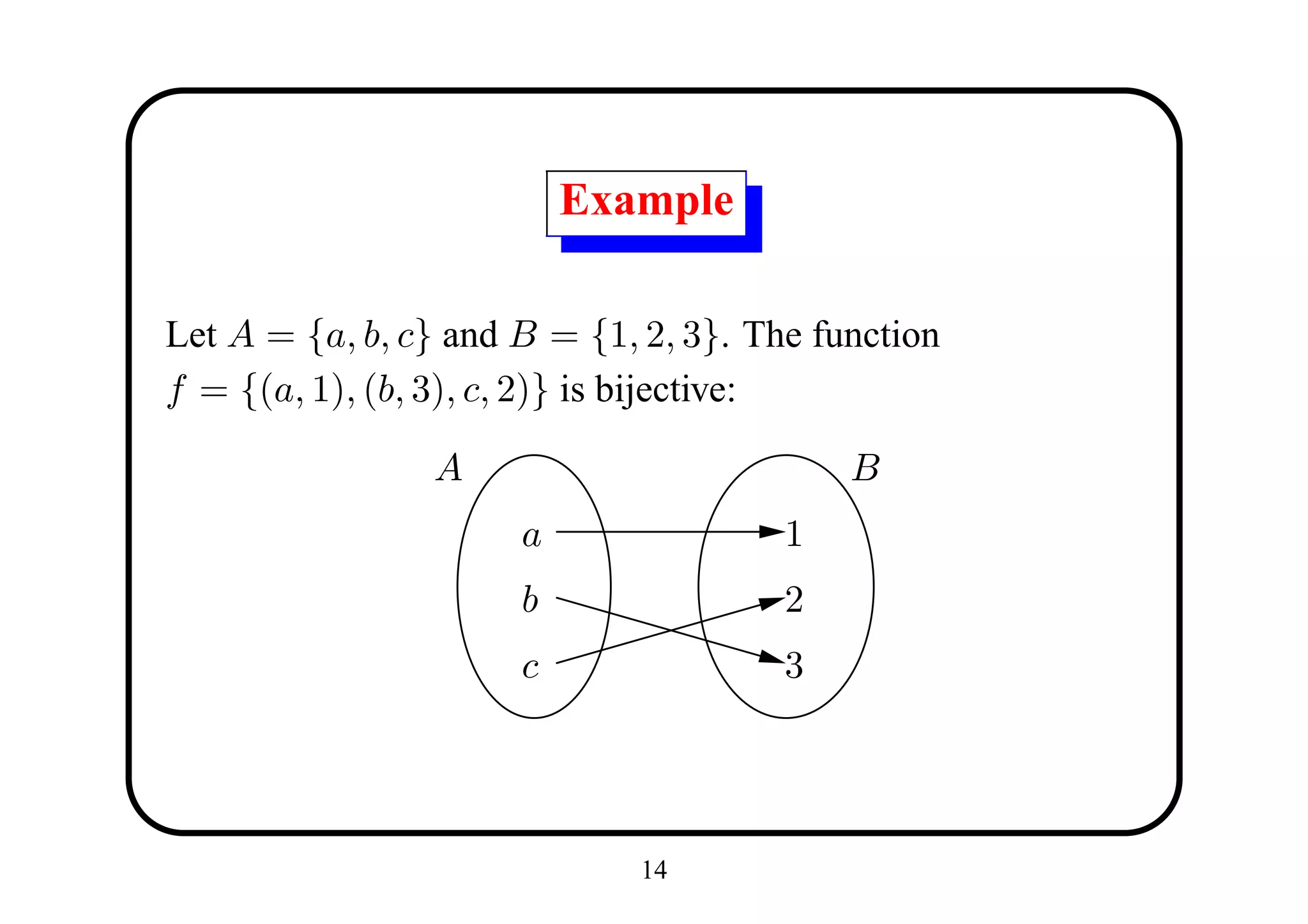
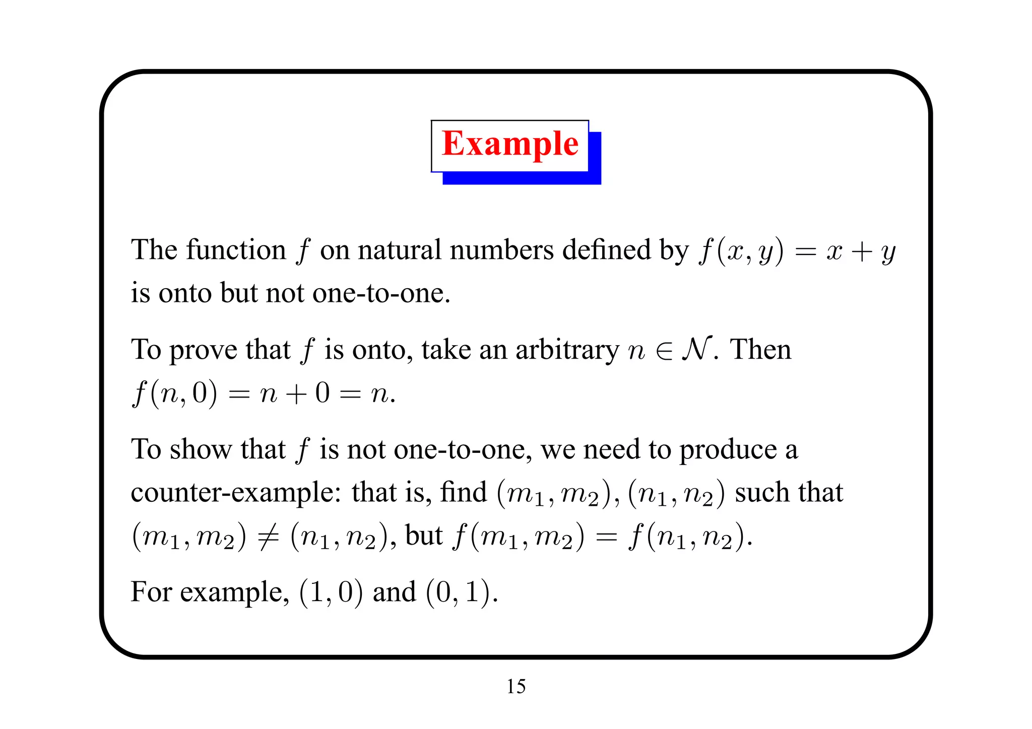
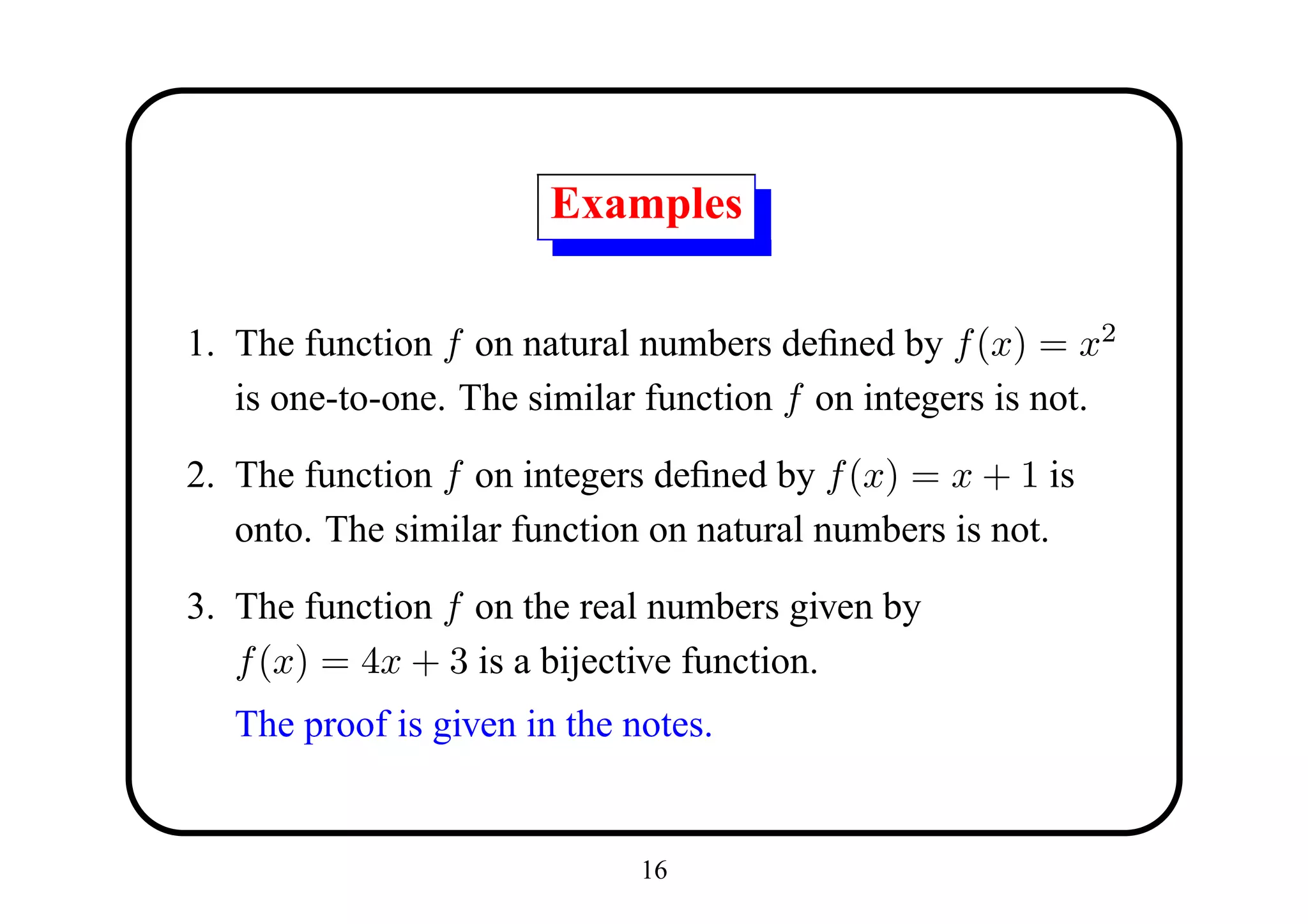
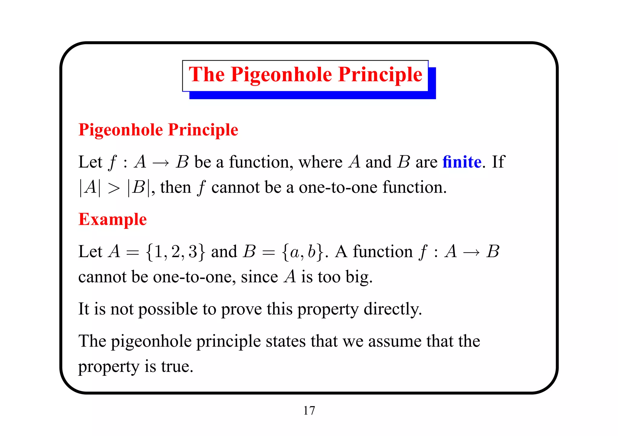
The document introduces functions and some of their properties. It defines a function as a relation where each element in the domain is mapped to exactly one element in the codomain. It discusses one-to-one, onto, and bijective functions. It also covers composition, associativity, identity functions, and the pigeonhole principle as it relates to functions between finite sets.

1. Functions
1

2. Introducing Functions
A function f from a set A to a set B, written f : A → B, is a
relation f ⊆ A × B such that every element of A is related to
one element of B; in logical notation
1. (a, b1 ) ∈ f ∧ (a, b2 ) ∈ f ⇒ b1 = b2 ;
2. ∀a ∈ A. ∃b ∈ B. (a, b) ∈ f .
The set A is called the domain and B the co-domain of f .
If a ∈ A, then f (a) denotes the unique b ∈ B st. (a, b) ∈ f .
2

3. Comments
If the domain A is the n-ary product A1 × . . . × An , then we
often write f (a1 , . . . , an ) instead of f ((a1 , . . . , an )).
The intended meaning should be clear from the context.
Recall the difference between the following two Haskell
functions:
f :: A -> B -> C -> D
f :: (A,B,C) -> D
Our definition of function is not curried.
3

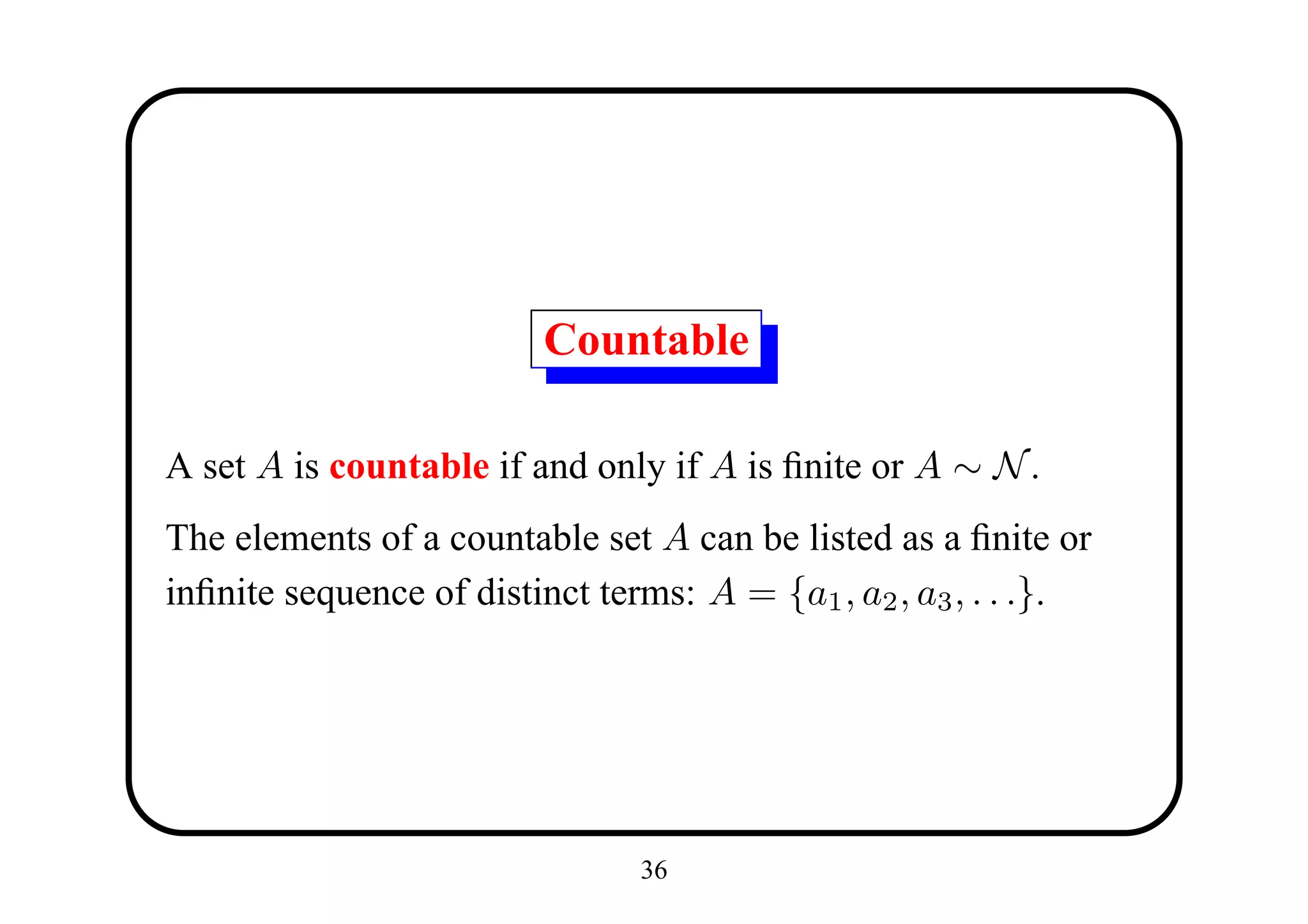
4. Image Set
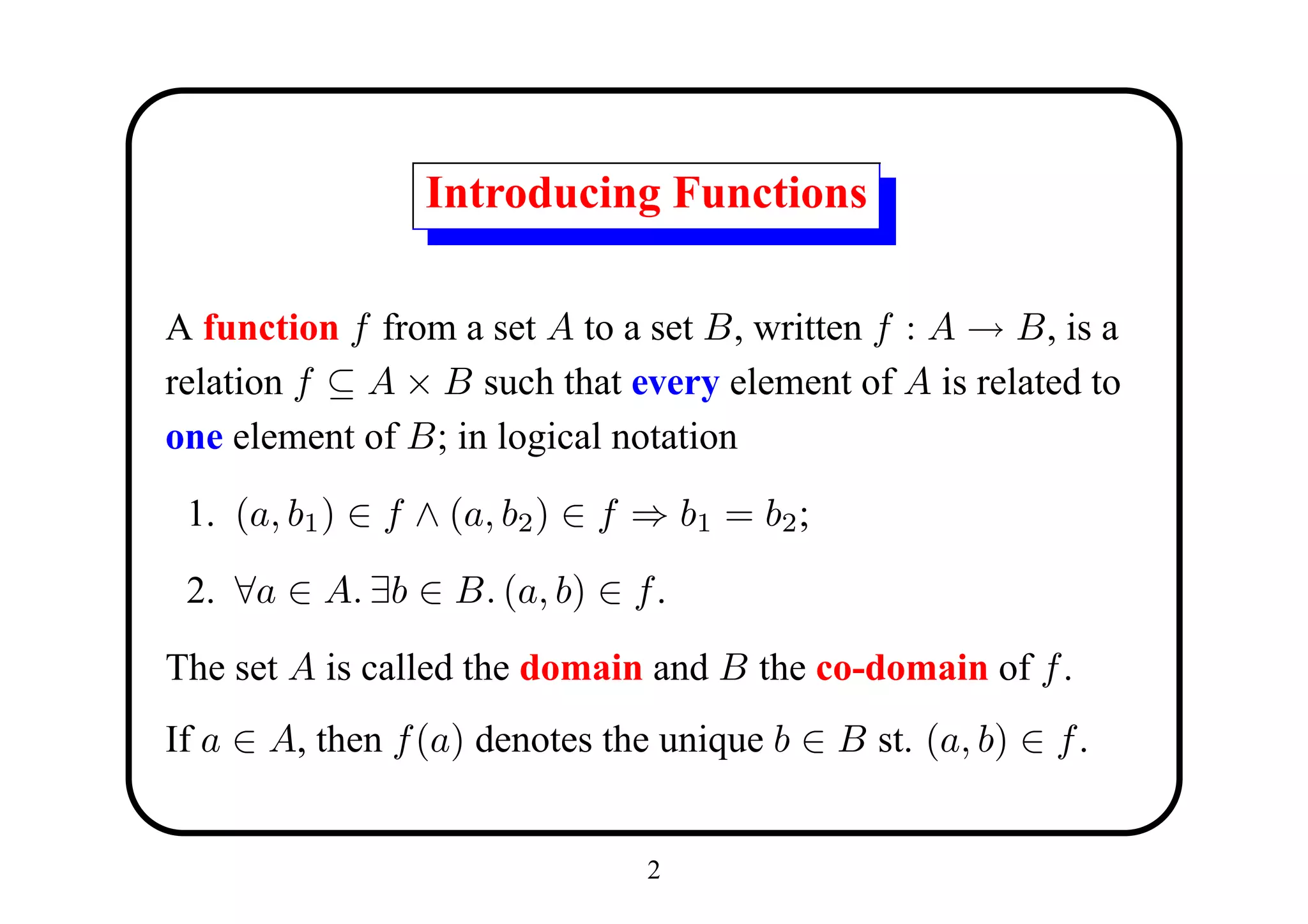
Let f : A → B. For any X ⊆ A, define the image of X under
f to be
def
f [X] = {f (a) : a ∈ X}
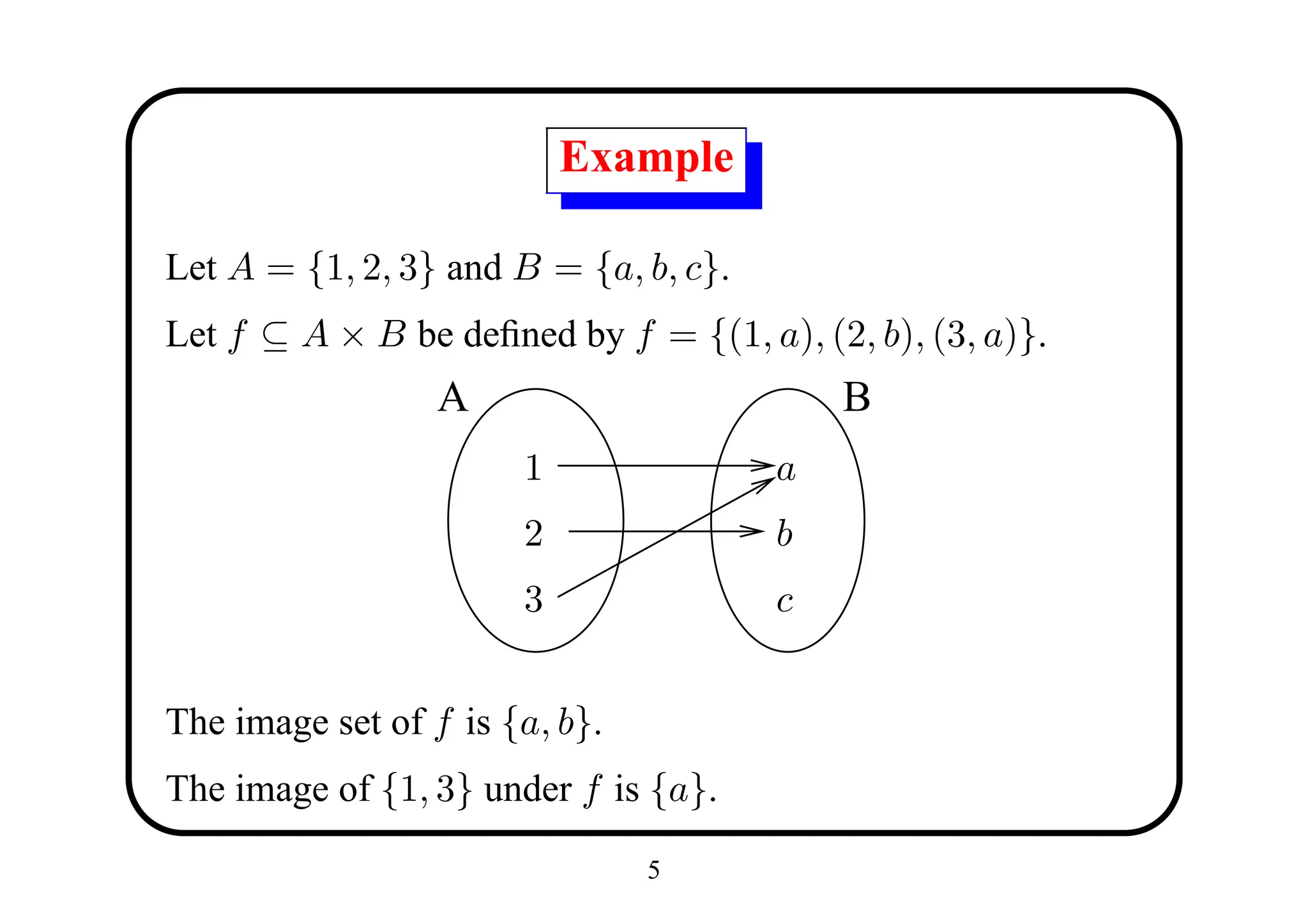
The set f [A] is called the image set of f .
4

5. Example
Let A = {1, 2, 3} and B = {a, b, c}.
Let f ⊆ A × B be defined by f = {(1, a), (2, b), (3, a)}.
A B
1 a
2 b
3 c
The image set of f is {a, b}.
The image of {1, 3} under f is {a}.
5

6. Example
Let A = {1, 2, 3} and B = {a, b}. Let f ⊆ A × B be defined
by f = {(1, a), (1, b), (2, b), (3, a)}.
This f is not a well-defined function.
A B
1 a
2
b
3
6

7. Examples
The following are examples of functions with infinite domains
and co-domains:
1. the function f : N × N → N defined by f (x, y) = x + y;
2. the function f : N → N defined by f (x) = x2 ;
3. the function f : R → R defined by f (x) = x + 3.
The binary relation R on the reals defined by x R y if and only
if x = y 2 is not a function
7

8. Cardinality
Let A → B denote the set of all functions from A to B, where
A and B are finite sets. If |A| = m and |B| = n, then
|A → B| = nm .
Sketch proof
For each element of A, there are n independent ways of
mapping it to B.
You do not need to remember this proof.
8

9. Partial Functions
A partial function f from a set A to a set B, written
f :A B, is a relation f ⊆ A × B such that just some
elements of A are related to unique elements of B:
(a, b1 ) ∈ f ∧ (a, b2 ) ∈ f ⇒ b1 = b2 .
The partial function f is regarded as undefined on those
elements which do not have an image under f .
We call this undefined value ⊥ (pronounced bottom).
A partial function from A to B is a function from A to
(B + {⊥}).
9

10. Examples of Partial Functions
1. Haskell functions which return run-time errors on some (or
all) arguments.
2. The relation R = {(1, a), (3, a)} ⊆ {1, 2, 3} × {a, b}:
A B
1 a
2
b
3
Not every element in A maps to an element in B.
√
3. The binary relation R on R defined by x R y iff x = y.
It is not defined when x is negative.
10

11. Properties of Functions
Let f : A → B be a function.
1. f is onto if and only if every element of B is in the image
of f :
∀b ∈ B. ∃a ∈ A. f (a) = b.
2. f is one-to-one if and only if for each b ∈ B there is at
most one a ∈ A with f (a) = b:
∀a, a ∈ A. f (a) = f (a ) implies a = a .
3. f is a bijection iff f is both one-to-one and onto.
11

12. Example
Let A = {1, 2, 3} and B = {a, b}. The function
f = {(1, a), (2, b), (3, a)} is onto, but not one-to-one:
A B
1 a
2 b
3
We cannot define a one-to-one function from A to B. There are
too many elements in A for them to map uniquely to B.
12

13. Example
Let A = {a, b} and B = {1, 2, 3}. The function
f = {(a, 3), (b, 1)} is one-to-one, but not onto:
a 1
2
b
3
It is not possible to define an onto function from A to B. There
are not enough elements in A to map to all the elements of B.
13

14. Example
Let A = {a, b, c} and B = {1, 2, 3}. The function
f = {(a, 1), (b, 3), c, 2)} is bijective:
A B
a 1
b 2
c 3
14

15. Example
The function f on natural numbers defined by f (x, y) = x + y
is onto but not one-to-one.
To prove that f is onto, take an arbitrary n ∈ N . Then
f (n, 0) = n + 0 = n.
To show that f is not one-to-one, we need to produce a
counter-example: that is, find (m1 , m2 ), (n1 , n2 ) such that
(m1 , m2 ) = (n1 , n2 ), but f (m1 , m2 ) = f (n1 , n2 ).
For example, (1, 0) and (0, 1).
15

16. Examples
1. The function f on natural numbers defined by f (x) = x2
is one-to-one. The similar function f on integers is not.
2. The function f on integers defined by f (x) = x + 1 is
onto. The similar function on natural numbers is not.
3. The function f on the real numbers given by
f (x) = 4x + 3 is a bijective function.
The proof is given in the notes.
16

17. The Pigeonhole Principle
Pigeonhole Principle
Let f : A → B be a function, where A and B are finite. If
|A| > |B|, then f cannot be a one-to-one function.
Example
Let A = {1, 2, 3} and B = {a, b}. A function f : A → B
cannot be one-to-one, since A is too big.
It is not possible to prove this property directly.
The pigeonhole principle states that we assume that the
property is true.
17

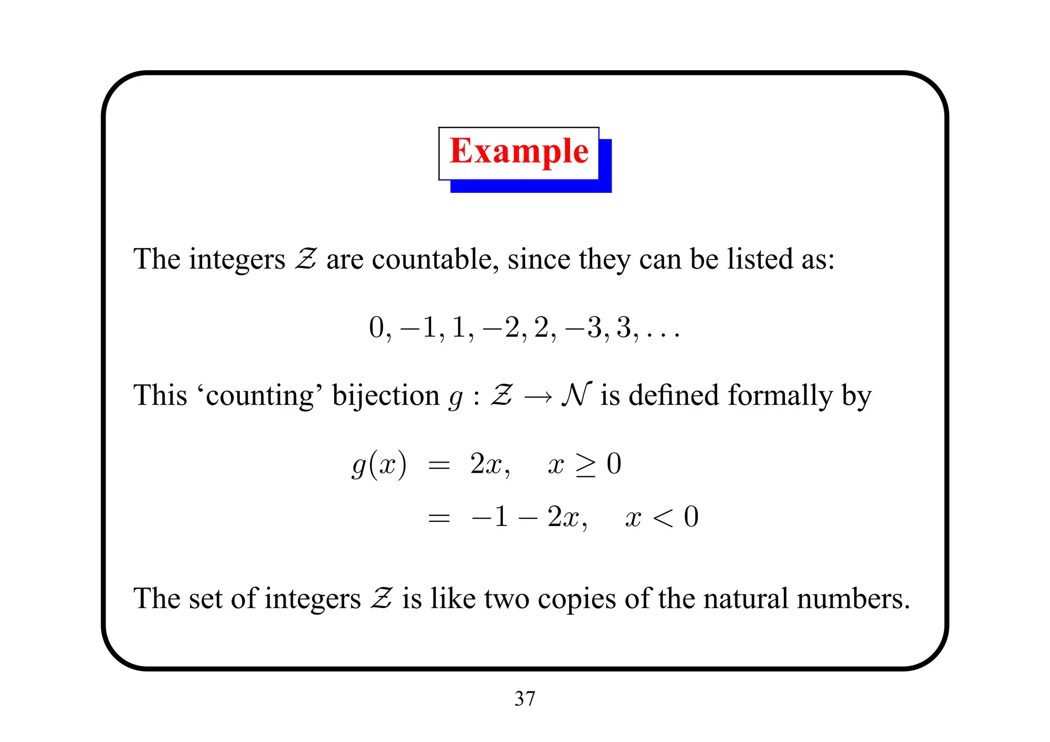
18. Proposition
Let A and B be finite sets, let f : A → B and let X ⊆ A. Then
|f [X]| ≤ |X|.
Proof Suppose for contradiction that |f [X]| > |X|. Define a
function p : f [X] → X by
p(b) = some a ∈ X such that f (a) = b.
There is such an a by definition of f [X]. We are placing the
members of f [X] in the pigeonholes X. By the pigeonhole
principle, there is some a ∈ X and b, b ∈ f [X] with
p(b) = p(b ) = a. But then f (a) = b and f (a) = b .
Contradiction.
18

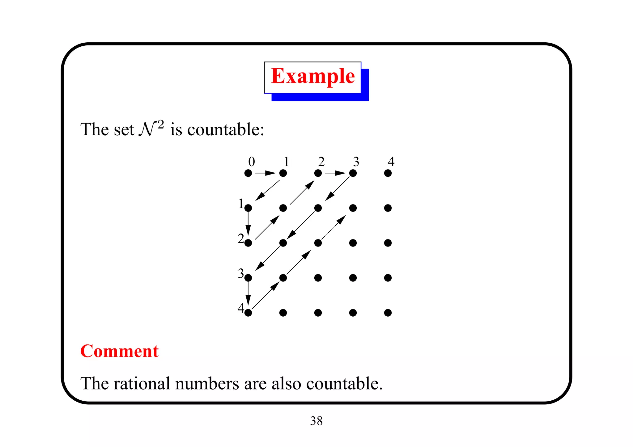
19. Proposition
Let A and B be finite sets, and let
f : A → B.
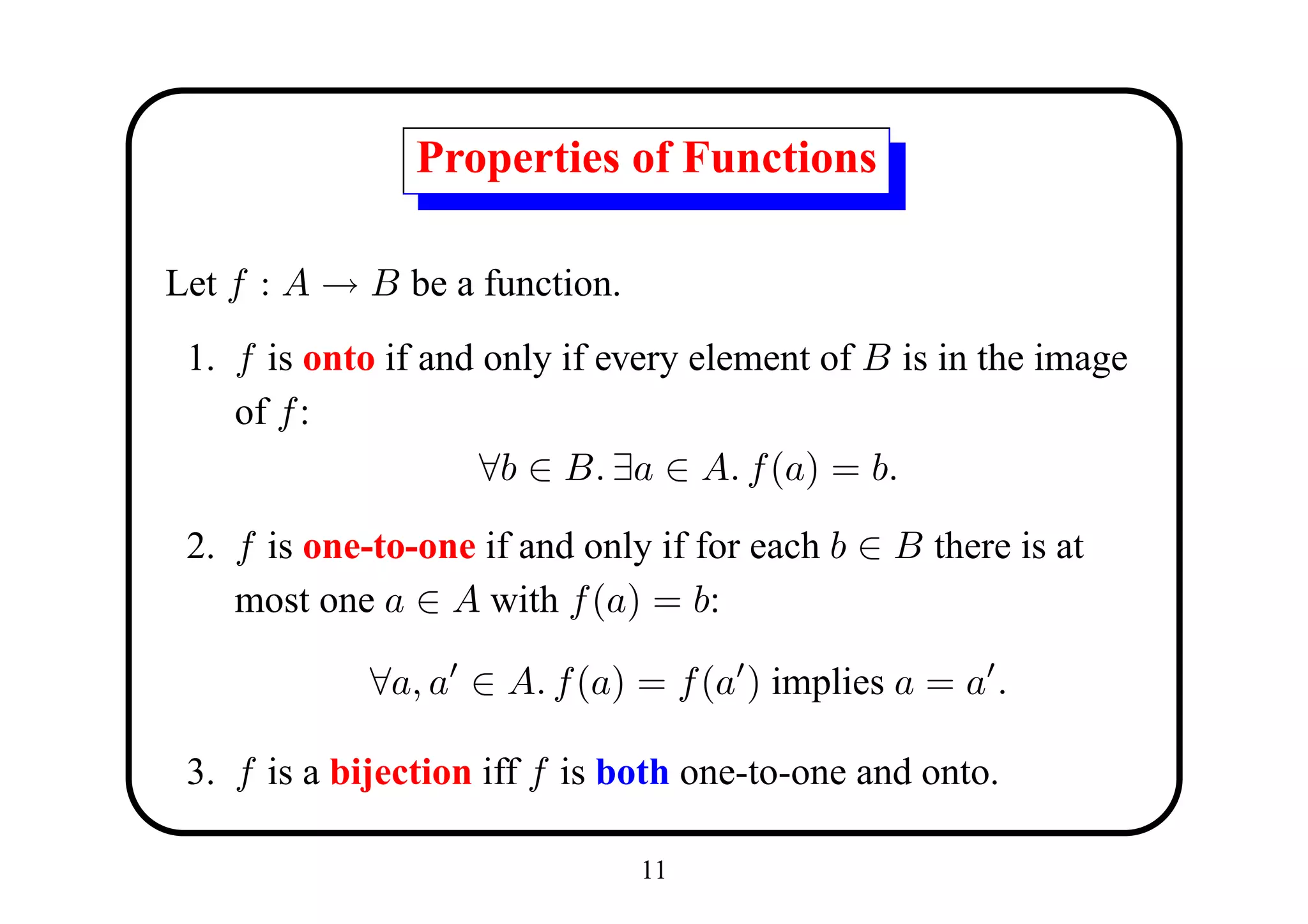
1. If f is one-to-one, then |A| ≤ |B|.
2. If f is onto, then |A| ≥ |B|.
3. If f is a bijection, then |A| = |B|.
19
Proof
Part (a) is the contrapositive of the
pigeonhole principle.
For (b), notice that if f is onto then
f [A] = B. Hence, |f [A]| = |B|. Also
|A| ≥ |f [A]| by previous proposition.
Therefore |A| ≥ |B| as required.
Part (c) follows from parts (a) and (b).

20. Composition
Let A, B and C be arbitrary sets, and let f : A → B and
g : B → C be functions.
The composition of f with g, written g ◦ f : A → C, is a
function defined by
def
g ◦ f (a) = g(f (a))
for every element a ∈ A. In Haskell notation, we would write
(g.f) a = g (f a)
It is easy to check that g ◦ f is indeed a function.
The co-domain of f must be the same as the domain of g.
20

21. Example
Let A = {1, 2, 3}, B = {a, b, c}, f = {(1, a), (2, b), (3, a)}
and g = {(a, 3), (b, 1)}.
Then g ◦ f = {(1, 3), (2, 1), (3, 3)}.
A B A
1 a 1
2 2
b
3 3
21

22. Associativity
Let f : A → B, g : B → C and h : C → D be arbitrary
functions. Then h ◦ (g ◦ f ) = (h ◦ g) ◦ f .
Proof Let a ∈ A be arbitrary. Then
(h ◦ (g ◦ f ))(a) = h((g ◦ f )(a))
= h(g(f (a)))
= (h ◦ g)(f (a))
= ((h ◦ g) ◦ f )(a)
22

23. Proposition
Let f : A → B and g : B → C be arbitrary
bijections. Then g ◦ f is a bijection.
Proof It is enough to show that
1. if f, g are onto then so is g ◦ f ;
2. if f, g are one-to-one then so is g ◦ f .
Assume f and g are onto. Let c ∈ C. Since
23
g is onto, we can find b ∈ B such that
g(b) = c. Since f is onto, we can find
a ∈ A such that f (a) = b. Hence
g ◦ f (a) = g(f (a)) = g(b) = c.
Assume f and g are one-to-one. Let
a1 , a2 ∈ A such that g ◦ f (a1 ) = g ◦ f (a2 ).
Then g(f (a1 )) = g(f (a2 )). Since g is
one-to-one, f (a1 ) = f (a2 ). Since f is also
one-to-one, a1 = a2 .

24. Identity
Let A be a set. Define the identity function on A, denoted
idA : A → A, by idA (a) = a for all a ∈ A.
In Haskell, we would declare the function
id :: A -> A
id x = x
24

25. Inverse
Let f : A → B be an arbitrary function. The function
g : B → A is an inverse of f if and only if
for all a ∈ A, g(f (a)) = a
for all b ∈ B, f (g(b)) = b
Another way of stating the same property is that g ◦ f = idA
and f ◦ g = idB .
25

26. Examples
1. The inverse relation of the function f : {1, 2} → {1, 2}
defined by f (1) = f (2) = 1 is not a function.
When an inverse function exists, it corresponds to the
inverse relation.
2. Let A = {a, b, c}, B = {1, 2, 3},
f = {(a, 1), (b, 3), (c, 2)} and g = {(1, a), (2, c), (3, b)}.
Then g is an inverse of f .
26

27. Proposition
Let f : A → B be a bijection, and define f −1 : B → A by
f −1 (b) = a whenever f (a) = b
The relation f −1 is a well-defined function.
It is the inverse of f (as shown in next proposition).
Proof
Let b ∈ B. Since f is onto, there is an a such that f (a) = b.
Since f is one-to-one, this a is unique. Thus f −1 is a function.
It satisfies the conditions for being an inverse of f .
27

28. Proposition
Let f : A → B. If f has an inverse g, then f must be a
bijection and the inverse is unique.
Proof To show that f is onto, let b ∈ B. Since f (g(b)) = b, it
follows that b must be in the image of f .
To show that f is one-to-one, let a1 , a2 ∈ A. Suppose
f (a1 ) = f (a2 ). Then g(f (a1 )) = g(f (a2 )). Since
g ◦ f = idA , it follows that a1 = a2 .
To show that the inverse is unique, suppose that g, g are both
inverses of f . Let b ∈ B. Then f (g(b)) = f (g (b)) since g, g
are inverses. Hence g(b) = g (b) since f is one-to-one.
28

29. Example
Consider the function f : N → N defined by
f (x) = x + 1, x odd
= x − 1, x even
It is easy to check that (f ◦ f )(x) = x, considering the cases
when x is odd and even separately. Therefore f is its own
inverse, and we can deduce that it is a bijection.
29

30. Cardinality of Sets
Definition
For any sets A, B, define A ∼ B if and only if there is bijection
from A to B.
Proposition Relation ∼ is reflexive, symmetric and transitive.
Proof Relation ∼ is reflexive , as idA : A → A is a bijection.
To show that it is symmetric, A ∼ B implies that there is a
bijection f : A → B. By previous proposition, it follows that f
has an inverse f −1 which is also a bijection. Hence B ∼ A.
The fact that the relation ∼ is transitive follows from previous
proposition.
30

31. Example
Let A, B, C be arbitrary sets, and consider the products
(A × B) × C and A × (B × C).
There is a natural bijection f : (A × B) × C → A × (B × C):
f : ((a, b), c) → (a, (b, c))
Also define the function g : A × (B × C) → (A × B) × C:
g : (a, (b, c)) → ((a, b), c)
Function g is the inverse of f .
31

32. Example
Consider the set Even of even natural numbers.
There is a bijection between Even and N given by f (n) = 2n.
Not all functions from Even to N are bijections.
The function g : Even → N given by g(n) = n is one-to-one
but not onto.
To show that Even ∼ N , it is enough to show the existence of
such a bijection.
32

33. Example
Recall that the cardinality of a finite set is the number of
elements in that set. Let |A| = n. There is a bijection
cA : {1, 2, . . . , n} → A.
Let A and B be two finite sets. If A and B have the same
number of elements, we can define a bijection f : A → B by
f (a) = (cB ◦ c−1 )(a).
A
Two finite sets have the same number of elements if and only if
there is a bijection between then.
33

34. Cardinality
Given two arbitrary sets A and B, then A has the same
cardinality as B, written |A| = |B|, if and only if A ∼ B.
Notice that this definition is for all sets.
34

35. Exploring Infinite Sets
The set of natural numbers is one of the simplest infinite sets.
We can build it up by stages:
0
0, 1
0, 1, 2
...
Infinite sets which can be built up in finite portions by stages
are particularly nice for computing.
35

36. Countable
A set A is countable if and only if A is finite or A ∼ N .
The elements of a countable set A can be listed as a finite or
infinite sequence of distinct terms: A = {a1 , a2 , a3 , . . .}.
36

37. Example
The integers Z are countable, since they can be listed as:
0, −1, 1, −2, 2, −3, 3, . . .
This ‘counting’ bijection g : Z → N is defined formally by
g(x) = 2x, x≥0
= −1 − 2x, x<0
The set of integers Z is like two copies of the natural numbers.
37

38. Example
The set N 2 is countable:
0 1 2 3 4
1
2
3
4
Comment
The rational numbers are also countable.
38

39. Uncountable Sets
Cantor showed that there are uncountable sets.
An important example is the set of reals R.
Another example is the power set P(N ).
We cannot manipulate reals in the way we can natural numbers.
Instead, we use approximations: for example, the floating point
decimals of type Float in Haskell.
For more information, see Truss, section 2.4.
39