79196-134739-1-SM (Published journal)

Development of a Theoretical Model for Prediction
of Surface Roughness of Metallic Surfaces using
Acoustic Signals
S. P. Harisubramanyabalaji, C. A. Sribalaji, A. Vivek, G. Vigneshwaran, S. Abhishek,
R. Balamurugan and R. Panneer*
School of Mechanical Engineering, SASTRA University, Thanjavur-613401, Tamil Nadu, India; haribalaji94@gmail.
com, balajianand1994@gmail.com, vivekanandan321@gmail.com, nannilamvickky@gmail.com,
abhisheksrinivasan007@gmail.com, balamuruganremesh5@gmail.com,panneer@mech.sastra.edu
Abstract
Objectives:TodevelopatheoreticalmodeltopredictthesurfaceRoughness(Ra
)ofdifferentmetallicsurfacesusingacoustic
signals. Methods: Acoustic signals are generated with the help of dry friction contact between two metallic surfaces. In
this work, Cast iron and Mild Steel Samples from different machining processes are collected and the dry friction contact
is made with HSS and Tungsten Carbide Tools to generate the acoustic signals. The acoustic signals obtained through a
microphone are processed using MATLAB. Number of Samples versus Amplitude is plotted and then the resulting output is
plotted as Time versus Amplitude. Subsequently the external noises from the acoustic signals are removed to get a reliable
roughness value. Findings: The maximum amplitudes of the samples are tabulated and used for the deriving model for the
surface roughness prediction. Theoretical model of HSS with various machining processes samples is y = 1.6865 ln(x) +
8.9978. Theoretical model of Tungsten carbide with various machining processes samples is y = 6.302 ln(x) + 27.337. Both
the models are correlating with a trend line of 0.9. Application: This theoretical model can be used to predict the surface
roughness (Ra
) of metallic surfaces. This approach can be implemented in surface finish measuring devices.
Keywords: Acoustic Signals, Amplitude, Microphone, Metallic Surfaces, Surface Roughness
1. Introduction
Surface Roughness is the deviations in the direction of
the normal vector of a real surface from its ideal form.
Surface roughness determines the amount of friction
that will be produced when the machined objects are
employed in machineries. Hence, Surface Roughness
must be measured properly to ensure the function of the
surface. To find the roughness value of any surface, the
most widely used Surface Measurement Parameter is Ra
1,2
and hence the Ra
value is used in this research work. The
surface measurement techniques can be broadly classified
as “contact” methods3,4
and “non-contact” methods7–9
.
Talysurf,Dektak,RutherfordBackscatteringSpectroscopy,
Nanoindenter are some of the devices which operate on
the contact method. In these devices a probe is made to
traverse along the surface of the job. The deviation of the
probe in very small scale is plotted as a graph, which is
used to find the profile of the surface and hence calculate
the value of the roughness5,6
. The disadvantage of contact
method is that the sensitive probe wears out and breaks
easily if misused or used on a metal with high roughness.
The non-contact methods are Optical Microscopy, White
Light Interferometry8
, Atomic Force Microscopy, Surface
Topography, Confocal Microscopy, Image Processing11–16
etc. In these methods, a light source, mostly LASER9
is
made to fall on the surface of the job and the profile of
the job surface is generated using the light reflected from
the surface. The non-contact methods are expensive.
Hence the proposed method, though a contact method,
*Author for correspondence
Indian Journal of Science and Technology, vol 8(22), IPL0267, September 2015
ISSN (Print) : 0974-6846
ISSN (Online) : 0974-5645

Development of a Theoretical Model for Prediction of Surface Roughness of Metallic Surfaces using Acoustic Signals
Indian Journal of Science and Technology2 Vol 8 (22) | September 2015 | www.indjst.org
comparatively reduce the cost of measurement of the
surface roughness of the metal and predict Ra
value in
close proximity to a value as obtained by existing contact
and non-contact methods and also overcomes the disad-
vantages of the contact methods. It is also noted here that
measurement using dry friction contact can be made in
the areas of surfaces which are not functionally critical.
2. Methodology
Surfaces are generated by various machining processes10
such as Turning, Shaping, Grinding, etc. Sample jobs are
prepared by Shaping a Cast Iron Sample and Turning, and
Cylindrical Grinding of Mild Steel Samples with High
Speed Steel (HSS) and Tungsten Carbide Inserts as cutting
tools with pre-set cutting conditions. Three samples were
chosen one each from Shaping, Turning, and Cylindrical
Grinding because they will have distinctive surface rough-
ness values which will be very useful in correlating the
relationship between the amplitude of Acoustic Signals
and Surface Roughness. The surface roughness (Ra
) val-
ues of these samples were measured using a Surface
Roughness Testing Machine and the actual Ra
values were
noted (Table 1 and 2).
To obtain the acoustic signals, an experimental set
up was established where the samples were secured
horizontally on to a surface plate with a holding and
clamping arrangement. To generate sound, the same tools
which machined those surfaces were used which were
set at an angle of 45° to the sample surface. At this angle,
there will be a point contact between the two metals and
hence the cutting will be avoided. The sample length of
movement was considered within the range of 5 cm – 15
cm. When the tools were making a dry friction contact
with the sample surface and moved, sound waves were
generated which is captured using a microphone.
The microphone is selected in such a way that it
does not attenuate the sound signal. The microphone is
fixed at a distance of about 3cm from the metal con-
tact point which is kept constant for all the samples so
as to capture the sound with same intensity. The sound
recorded by the microphone includes the sound from
the surface, surrounding noises and some noise due
to the vibrations produced when the two metals are in
contact17
. Hence the entire set up was established in a
sound proof environment. To avoid the sound produced
by the vibrations due to the movement of the tool over
the surface, the sample was isolated from the base while
clamping. The sound is recorded in the form of .wma
format and is converted into .wav format to make it
readable in MATLAB. This .wav file is read in MATLAB
and the amplitude of the sound wave is plotted against
number of samples initially. The sampling frequency is
found to be 44100 samples per second18,19
. The X-axis
is then converted into time (in seconds) and the plot of
time vs. amplitude is obtained. The sound file is found
to be consisting of audio signals which are not a part
of the signals related to surface, but due to the place-
ment of tool over the work piece etc. These portions are
removed from the sound wave by observing the time
period of the unwanted signals. The default MATLAB
function of “max” which returns the maximum value
of amplitude from the signal is used for defining the
surface roughness.
3. Results
On testing these three samples with the above methodology
by dry friction of High Speed Steel and Tungsten Carbide
Inserts with the sample surfaces, sound signal were
obtained. The signals obtained were converted to plots
relating amplitude to time domain and then those signals
which are not part of the surface quality are removed. The
resulting plots are presented in Figures 1 to 6.
Table 1. Actual surface roughness (Ra
) versus max
amplitude of acoustic signal generated by HSS
NO Machining
Process
Measured Suface
Finish(Ra
)
Max. Amplitude
of Acoustic
Signal
1 Shaping 6.15 0.1373
2 Turning 3.97 0.0733
3 Cylindrical
Grinding
0.28 0.0053
Table 2. Actual surface roughness (Ra
) versus max
amplitude of acoustic signal generated by Tungsten
Carbide
NO
Machining
Process
Measured Suface
Finish(Ra
)
Max. Amplitude of
Acoustic
Signal
1 Shaping 6.15 0.0303
2 Turning 3.97 0.0284
3
Cylindrical
Grinding
0.28 0.0135

S. P. Harisubramanyabalaji, C. A. Sribalaji, A. Vivek, G. Vigneshwaran, S. Abhishek, R. Balamurugan and R. Panneer
Indian Journal of Science and Technology 3Vol 8 (22) | September 2015 | www.indjst.org
3.1 Details of Plots Generated by Dry
Friction of HSS on Three Surfaces
Produced by Shaping, Turning and
Grinding
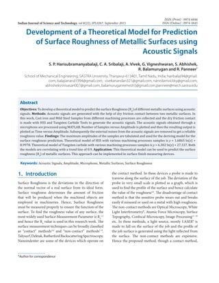
The details of the plots of the acoustic signals generated
during dry friction of High Speed Steel on Cast Iron
Sample shaped using Shaping Machine are presented above
in Figure 1a to 1c. The Figure 1a shows the acoustic sig-
nals plotted taking amplitude along Y-axis and number of
samples along X-axis. The plot converted into amplitude vs.
time grid is shown in Figure 1b. The plot showing the signal
after removing unwanted signal is shown Figure 1c, As can
be observed from Figure 1c the max. amplitude of the sig-
nal is 0.1373 (Obtained from MATLAB max. function).
The details of the plots of the acoustic signals generated
duringdryfrictionofHighSpeedSteelonCylindricalMild
Steel Sample turned using Lathe Machine are presented
below in Figure 2a to 2c. The Figure 2a shows the acoustic
signals plotted taking amplitude along Y-axis and number
of samples along X-axis. The plot converted into amplitude
Figure 1. (a) Acoustic signals amplitude vs. samples (HSS
onCastIronSampleproducedinshaper),(b)Acousticsignals
amplitude vs. time (HSS on Cast Iron Sample produced
in shaper) and (c) Acoustic signals reflecting the surface
roughness (HSS on Cast Iron Sample produced in shaper).
(a)
(b)
(c)
on Mild Steel sample produced in Lathe), (b)Acoustic signals
amplitude vs. time (HSS on Mild Steel sample produced
in Lathe) and (c) Acoustic signals reflecting the surface
roughness (HSS on Mild Steel sample produced in Lathe).
(a)
(b)
(c)

samples along X-axis. The plot converted into amplitude
vs. time grid is shown in Figure 3b. The grid showing the
signal after removing those signals from the plot which are
not part of the intended sound waves and which reflects
only the surface roughness is shown Figure 3c. As can be
observed from Figure 3c the max amplitude of the signal
is 0.0053 (Obtained from MATLAB max function).
3.2 Details of Plots Generated by Dry
Friction of Tungsten Carbide on Three
Samples produced by Shaping, Turning
and Grinding
The details of the plots generated during dry friction of
Tungsten Carbide on Cast Iron Sample Shaped using
Shaping Machine are presented below in Figure 4a to 4c. The
Figure 4ashowstheacousticsignalsplottedtakingamplitude
along Y-axis and number of samples along X-axis. The plot
converted into amplitude vs. time grid is shown in Figure
4b. The plot showing the signal after removing those signals
which are not part of the intended sound waves and which
reflects only the surface roughness is shown Figure 1c. As
can be observed from Figure 4c the max amplitude of the
signal is 0.0303 (Obtained from MATLAB max function).
The details of the plots generated during dry friction of
TungstenCarbideonCylindricalMildSteelSampleturned
using Lathe Machine are presented below in Figure 5a to
5c. The Figure 5a shows the acoustic signals plotted tak-
ing amplitude along Y-axis and number of samples along
X-axis. The plot converted into amplitude vs. time grid
is shown in Figure 5b. The grid showing the signal after
removing those signals from the plot which are not part
of the intended sound waves and which reflects only the
surface roughness is shown Figure 5c. As can be observed
from Figure 5c the max amplitude of the signal is 0.0284
(Obtained from MATLAB max function).
The details of the plots generated during dry friction
of Tungsten Carbide on Cylindrical Mild Steel Sample
ground using Grinding Machine are presented below in
Figure 6a to 6c. The Figure 6a shows the acoustic signals
plotted taking amplitude along Y-axis and number of
samples along X-axis. The plot converted into amplitude
observed from Figure 6c the max amplitude of the signal
is 0.0135 (Obtained from MATLAB max function).
observed from Figure 2c the max. amplitude of the signal
is 0.0733, (Obtained from MATLAB max function).
The details of the plots generated during dry friction
of High Speed Steel on Cylindrical Mild Steel Sample
ground using Grinding Machine are presented below in
Figure 3a to 3c. The Figure 3a shows the acoustic signals
plotted taking amplitude along Y-axis and number of
(a)
(b)
(c)
on Mild Steel Sample produced in Grinding Machine).
(b) Acoustic signals amplitude vs. time (HSS on Mild Steel
Sample produced in Grinding Machine). (c) Acoustic signals
reflecting the surface roughness (HSS on Mild Steel Sample
produced in Grinding Machine).

roughness and the amplitudes of signals. This correlation
can be effectively used to develop a theoretical model to
predict surface roughness from the acoustic signals.
5. Theoretical Model
To develop a theoretical model relating the surface
roughness and the observed amplitude, a logarithmic trend
line20,21
was formed with Maximum Amplitude in X-axis
Figure 5. (a) Acoustic Signals Amplitude vs. samples
(Tungsten Carbide on Mild Steel sample produced in Lathe),
(b) Acoustic Signals Amplitude vs. Time (Tungsten Carbide
on Mild Steel sample produced in Lathe) and (c) Acoustic
Signals reflecting the surface roughness (Tungsten Carbide
on Mild Steel sample produced in Lathe).
Figure 4. (a) Acoustic signals amplitude vs. samples
(Tungsten Carbide on Cast Iron Sample produced in shaper),
(b) Acoustic signals amplitude vs. time (Tungsten Carbide
on Cast Iron Sample produced in shaper) and (c) Acoustic
signals reflecting the surface roughness (Tungsten Carbide
on Cast Iron Sample produced in shaper).
(a)
(b)
(c)
4. Summary and Results
The values of maximum amplitudes were tabulated against
the corresponding actually measured Ra
value. Table 1
presents the details of the amplitudes generated by HSS
on different samples against the actually measured sur-
face finish and Table 2 presents the details of amplitudes
generated by Tungsten Carbide on different samples
against the actually measured surface finish.
As can be observed from Table 1 and 2 there is a good
correlation between the variance in the measured surface
(a)
(b)
(c)

and Surface Roughness in Y-axis (Figure 7). When such
a trend line was formed using the appropriate feature in
Excel for the combination of High Speed Steel versus vari-
ous samples, the equation relating them was found to be,
y = 1.6865 ln(x) + 8.9978 (1)
Where x represents the maximum amplitude and y
represents the surface roughness. Similarly another trend
line was formed for the combination of Tungsten Carbide
versus various samples (Figure 8); the equation relating
them was found to be
y = 6.302 ln(x) + 27.337 (2)
Based on the above logarithmic trend line equations,
the surface roughness of a machined surface can be pre-
dicted according to the type of combinations of material
being used to make the dry friction.
6. Conclusion
The above results show that the acoustic signals produced
by the pair of HSS with other metals and pair of Tungsten
Carbide with other metals vary in frequency and
correlations.
The maximum value of the amplitude is taken and
correlated to get the corresponding equations from which
the surface roughness of the material can be predicted.
Two different equations are obtained for HSS and
Tungsten Carbide which can be used for prediction of
(a)
(b)
(c)
Figure 6. (a) Acoustic Signals Amplitude vs. samples
Carbide on Mild Steel ground in Grinding Machine),
(b) Acoustic Signals Amplitude vs. Time (Carbide on Mild
Steel ground in Grinding Machine) and (c) Acoustic Signals
reflecting the surface roughness (Carbide on Mild Steel
ground in Grinding Machine).
Figure 7. Trend Line - Log Surface Finish vs. Amplitude
(For HSS versus various samples).
Figure 8. Trend Line - Log Surface Finish vs. Amplitude
(For Tungsten Carbide versus various samples).

the surface roughness of any material pair, provided one
material in the pair is HSS or Carbide.
Thus,thismethodcanbeimplementedonanymaterial
pair to find the corresponding equation for the selected
materials to predict surface roughness of the materials.
This method is a simple and a cheaper method to
predict surface roughness compared to other costlier
methods and instruments.
This method’s limitations are that it needs sound proof
environment, other disturbances may influence the signal
and we need to identify and filter the intended signal from
other unwanted signal.
7. Acknowledgement
The work described in this paper was completed with
the support of School of Mechanical Engineering and
the School of Electrical and Electronics Engineering of
SASTRA University, Thanjavur, Tamilnadu, India.
8. References
1. Benardos PG, Vosniakos GC. Predicting surface roughness
in machining: A review. International Journal of Machine
Tools and Manufacture. 2003 Jun; 43(8):833–44.
2. Elmas S, Islam N, Jackson MR, Parkin RM. Analysis of
profile measurement techniques employed to surfaces
planed by an active machining system. Measurement. 2011
Feb; 44(2):365–77.
3. Mignot J, Gorecki C. Measurement of surface roughness:
Comparison between a defect-of-focus optical tech-
nique and the classical stylus technique. Wear. 1983 May;
87(1):39–49.
4. Arvinth Davinci M, Parthasarathi NL, Borah U, Albert SK.
Effect of the tracing speed and span on roughness param-
eters determined by stylus type equipment. Measurement.
2014 Feb; 48:368–77.
5. Tanneer LH. A comparison between Talysurf and optical
measurements of roughness and surface slope. Wear. 1979
Nov; 57(1):81–91.
6. Figgis DL, Sarkar AD. Wear results from Talysurf traces.
Wear. 1978 Dec; 51(2):317–26.
7. Bjuggren M, Krummenacher L, Mattsson L. Noncontact
surface roughness measurement of engineering surfaces by
total integrated infrared scattering. Precision Engineering.
1997 Jan; 20(1):33–45.
8. Devillez, Lesko S, Mozer W. Cutting tool crater wear
measurement with white light Interferometry. Wear. 2004
Jan; 256(1-2):56–65.
9. LeeS,KimSW,YimDY.Anin-processmeasurementtechnique
using laser for non-contact monitoring of surface rough-
ness and form accuracy of ground surfaces. CIRP Annals
- Manufacturing Technology. 1987; 36(1):425–428.
10. Bhuiyan MSH, Choudhury IA, Dahari M. Monitoring
the tool wear, surface roughness and chip formation
occurrences using multiple sensors in turning. add Journal
of Manufacturing Systems. 2014 Oct; 33(4):476–87.
11. Persson U. Measurement of surface roughness on rough
machined surfaces using spectral speckle correlation and
image analysis. Wear. 1993 Feb; 160(2):221–25.
12. Jeyapoovan T, Murugan M. Surface roughness classification
using image processing. Measurement. 2013 Aug;
46(7):2065–072.
13. Xiang HZ, Lei Z, Jiaxu T, Xuehong M, Xiaojun S.
Evaluation of three-dimensional surface roughness param-
eters based on digital image processing. The International
Journal of Advanced Manufacturing Technology. 2009 Jan;
40(3):342–8.
14. Pancewicz T, Mruk I. Holographic contouring for
determination of three-dimensional description of surface
roughness. Wear. 1996 Nov; 199(1):127–31.
15. Mitri FG, Kinnick RR, Greenleaf JF, Fatemi M.
Continuous-wave ultrasound reflectometry for surface
roughness imaging applications. Ultrasonics. 2009 Jan;
49(1):10–4.
16. Gao Z, Zhao X. Roughness measurement of moving
weak-scattering surface by dynamic speckle image. Optics
and Lasers in Engineering. 2012 May; 50(5):668–77.
17. Singh SK, Srinivasan K, Chakraborty D. Acoustic
characterization and prediction of surface roughness.
Guwahati, India Department of Mechanical Engineering,
Indian Institute of Technology. 2004 Oct; 152(2):127–30.
18. Hocheng H, Hsieh ML. Signal analysis of surface
roughness in diamond turning of lens molds. International
Journal of Machine Tools and Manufacture. 2004 Dec;
44(15):1607–18.
19. Chang W-R, Matz S. The effect of filtering processes on
surface roughness parameters and their correlation with
the measured friction, Part I: quarry tiles. Safety Science.
2000 Oct; 36(1):19–33.
20. Persson U. Surface roughness measurement on
machined surfaces using angular speckle correlation.
Journal of Materials Processing Technology. 2006 Dec;
180(1-3):233–38.
21. Liu JJ, Dornfeld DA, Dir AE. Correlating tool life, tool wear
and surface roughness by monitoring acoustic emission in
finish turning. Wear. 1992 Jan; 152(2):395–407.

79196-134739-1-SM (Published journal)

Recommended

Recommended

More Related Content

What's hot

What's hot (16)

Viewers also liked

Viewers also liked (11)

Similar to 79196-134739-1-SM (Published journal)

Similar to 79196-134739-1-SM (Published journal) (20)

79196-134739-1-SM (Published journal)