402064
ENGINEERING ANALYSIS
CHAPTER 1:FUNDAMENTALS OF LINEAR
SYSTEMS
Hoang Thi Huong Giang, PhD
.
TON DUC THANG UNIVERSITY
FACULTY OF ELECTRICAL & ELECTRONICS ENGINEERING
DEPARTMENT OF ELECTRONICS & TELECOMMUNICATIONS
2.
CHAPTER 1: FUNDAMENTALSOF
LINEAR SYSTEMS
1.1 Introduction
1.2 Linear algebra
1.3 Transfer function and impulse response
1.4 Representation of control systems
04/21/2025
402064-Chapter 1: Fundamentals of Linear
Systems 2
3.
OBJECTIVES
Understand thebasic concepts and
disciplines of automatic control.
Learn the different between classical and
modern modelling of control systems
Review the representation of linear control
systems
04/21/2025
402064-Chapter 1: Fundamentals of Linear
Systems 3
4.
CHAPTER 1: FUNDAMENTALSOF
LINEAR SYSTEMS
1.1 Introduction
1.2 Linear algebra
1.3 Transfer function and impulse response
1.4 Representation of control systems
04/21/2025
402064-Chapter 1: Fundamentals of Linear
Systems 4
5.
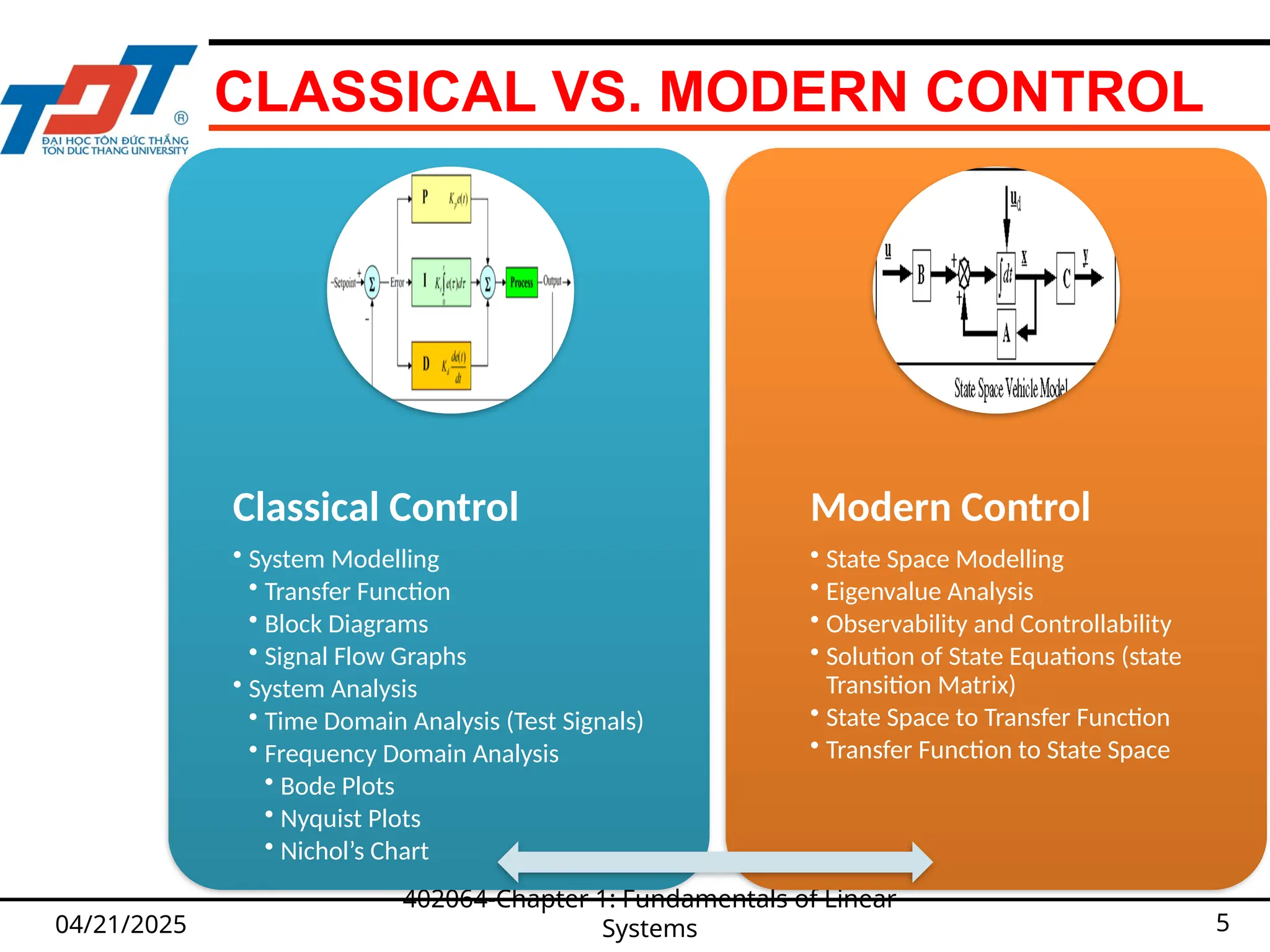
CLASSICAL VS. MODERNCONTROL
04/21/2025
402064-Chapter 1: Fundamentals of Linear
Systems 5
Classical Control
• System Modelling
• Transfer Function
• Block Diagrams
• Signal Flow Graphs
• System Analysis
• Time Domain Analysis (Test Signals)
• Frequency Domain Analysis
• Bode Plots
• Nyquist Plots
• Nichol’s Chart
Modern Control
• State Space Modelling
• Eigenvalue Analysis
• Observability and Controllability
• Solution of State Equations (state
Transition Matrix)
• State Space to Transfer Function
• Transfer Function to State Space
6.
WHAT IS ACONTROL SYSTEM?
04/21/2025
402064-Chapter 1: Fundamentals of Linear
Systems 6
Generally speaking, a control system is a
system that is used to realize a desired output
or objective.
Control systems are everywhere:
They appear in our homes, in cars, in industry, in
scientific labs, and in hospital…
Principles of control have an impact on diverse fields
as engineering, aeronautics ,economics, biology and
medicine…
Wide applicability of control has many advantages
(e.g., it is a good vehicle for technology transfer)
7.
WHAT DO THESETWO HAVE IN
COMMON?
04/21/2025
402064-Chapter 1: Fundamentals of Linear
Systems 7
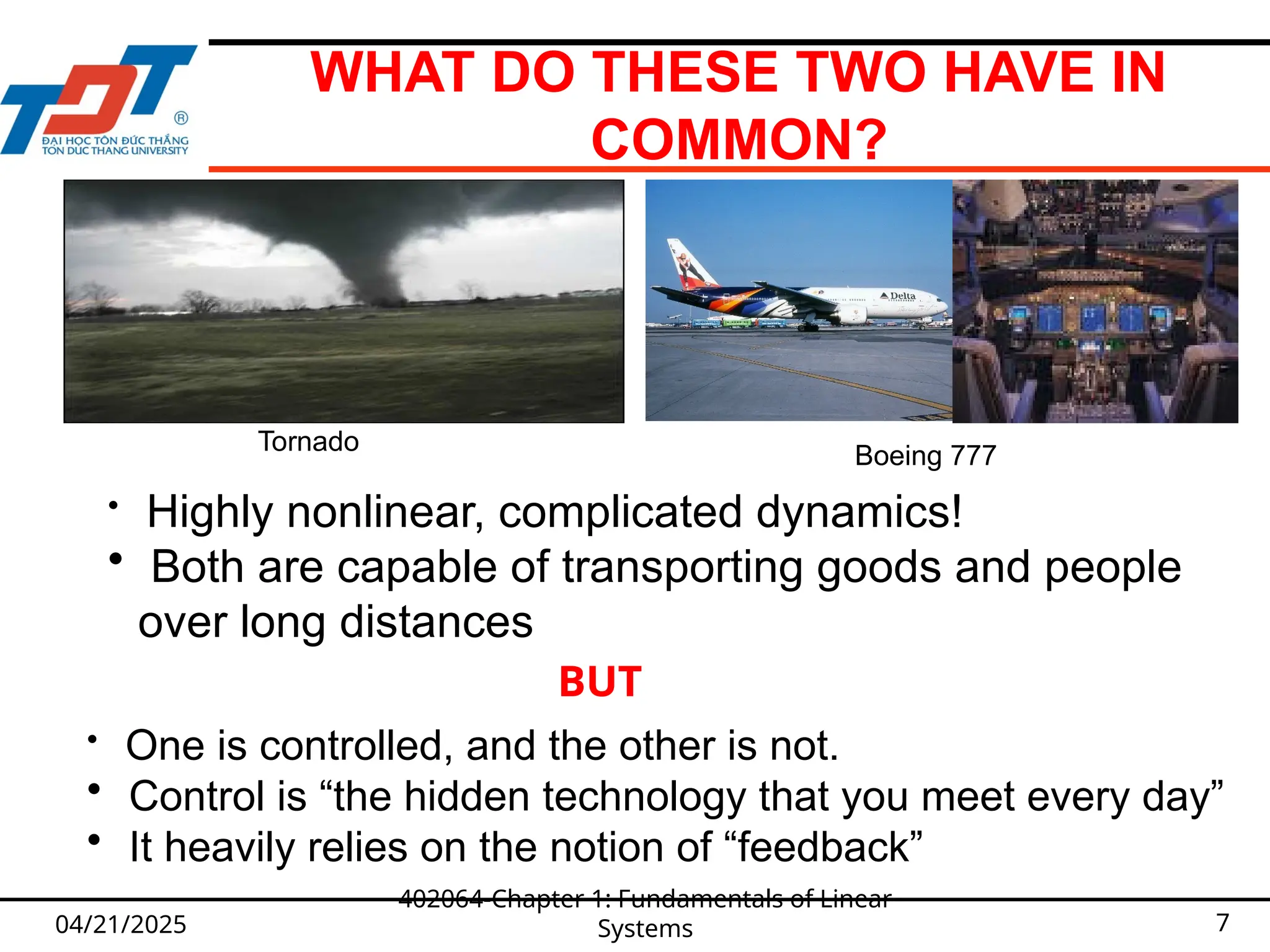
Tornado
Boeing 777
• Highly nonlinear, complicated dynamics!
• Both are capable of transporting goods and people
over long distances
BUT
• One is controlled, and the other is not.
• Control is “the hidden technology that you meet every day”
• It heavily relies on the notion of “feedback”
8.
DEFINITIONS
04/21/2025
402064-Chapter 1: Fundamentalsof Linear
Systems 8
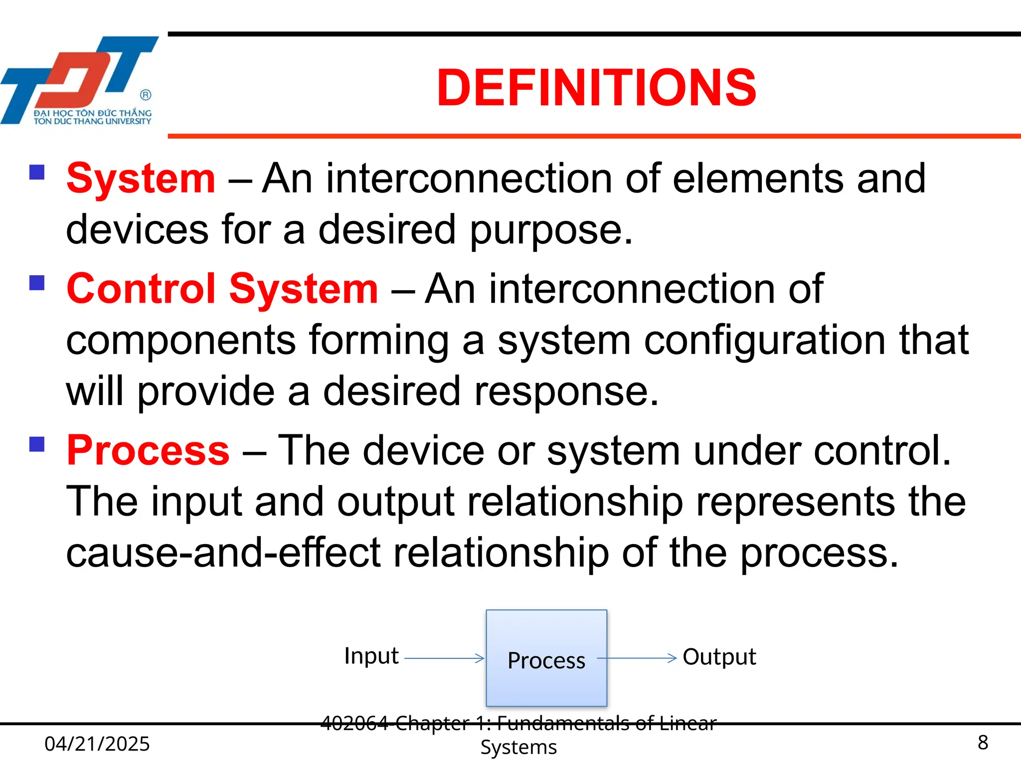
System – An interconnection of elements and
devices for a desired purpose.
Control System – An interconnection of
components forming a system configuration that
will provide a desired response.
Process – The device or system under control.
The input and output relationship represents the
cause-and-effect relationship of the process.
Process Output
Input
9.
DEFINITIONS
04/21/2025
402064-Chapter 1: Fundamentalsof Linear
Systems 9
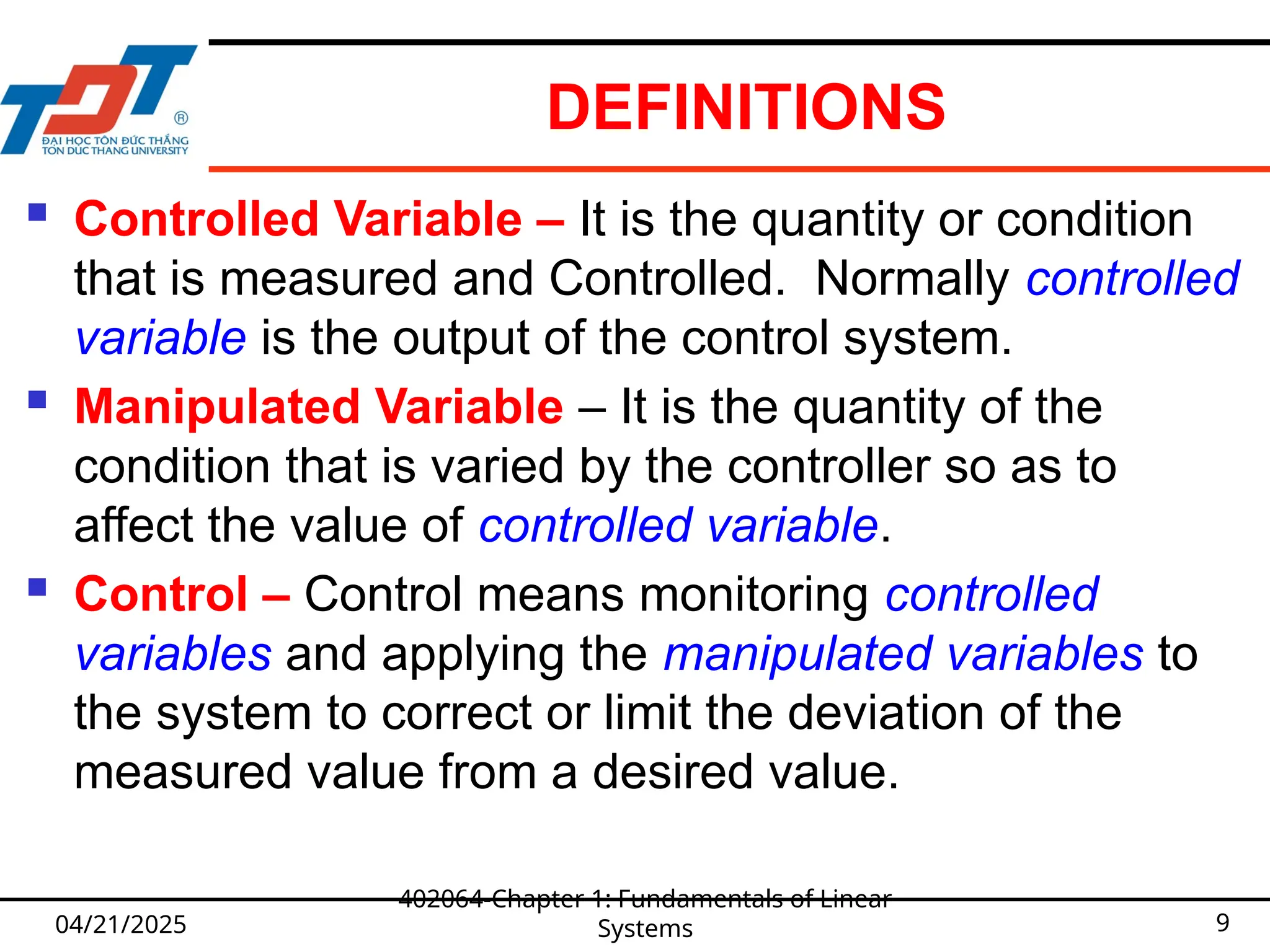
Controlled Variable – It is the quantity or condition
that is measured and Controlled. Normally controlled
variable is the output of the control system.
Manipulated Variable – It is the quantity of the
condition that is varied by the controller so as to
affect the value of controlled variable.
Control – Control means monitoring controlled
variables and applying the manipulated variables to
the system to correct or limit the deviation of the
measured value from a desired value.
10.
DEFINITIONS
04/21/2025
402064-Chapter 1: Fundamentalsof Linear
Systems 10
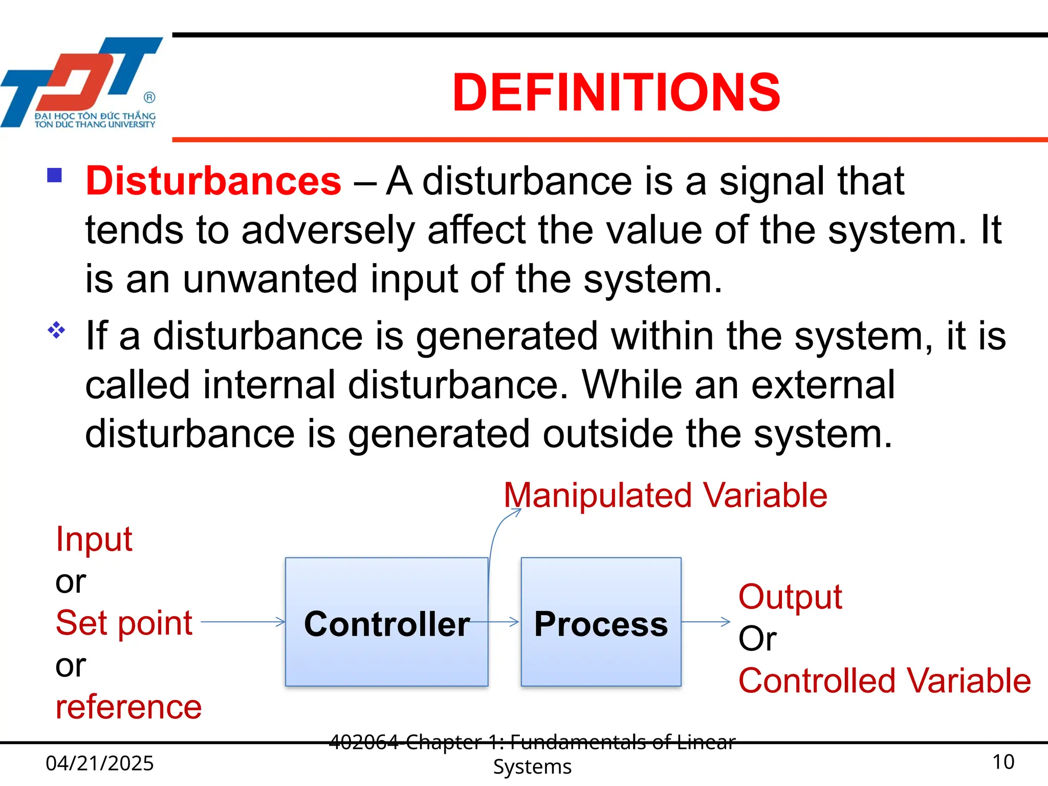
Disturbances – A disturbance is a signal that
tends to adversely affect the value of the system. It
is an unwanted input of the system.
If a disturbance is generated within the system, it is
called internal disturbance. While an external
disturbance is generated outside the system.
Controller
Output
Or
Controlled Variable
Input
or
Set point
or
reference
Process
Manipulated Variable
11.
BRIEF HISTORY OFCONTROL
04/21/2025
402064-Chapter 1: Fundamentals of Linear
Systems 11
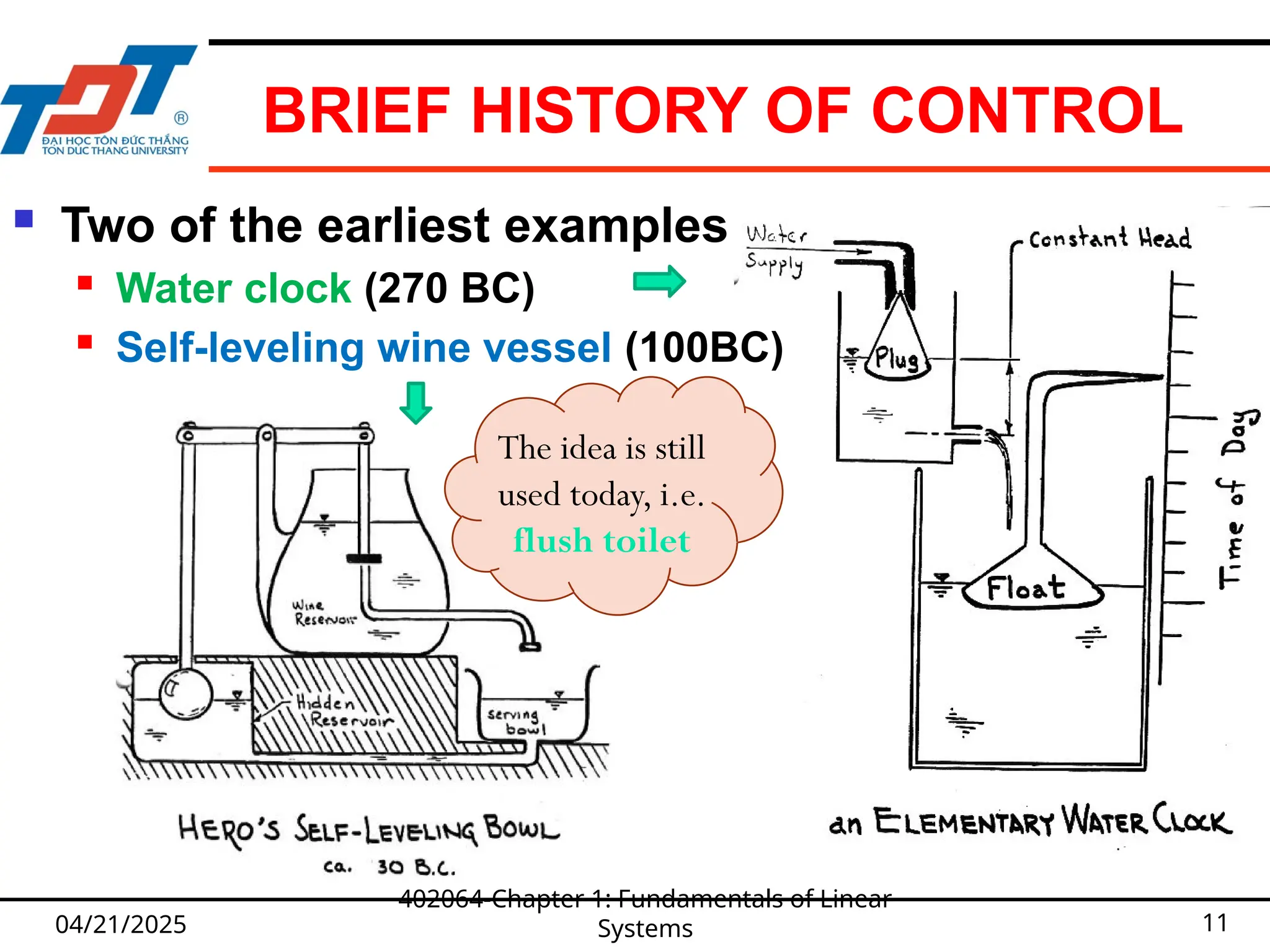
Two of the earliest examples
Water clock (270 BC)
Self-leveling wine vessel (100BC)
The idea is still
used today, i.e.
flush toilet
12.
BRIEF HISTORY OFCONTROL
04/21/2025
402064-Chapter 1: Fundamentals of Linear
Systems 12
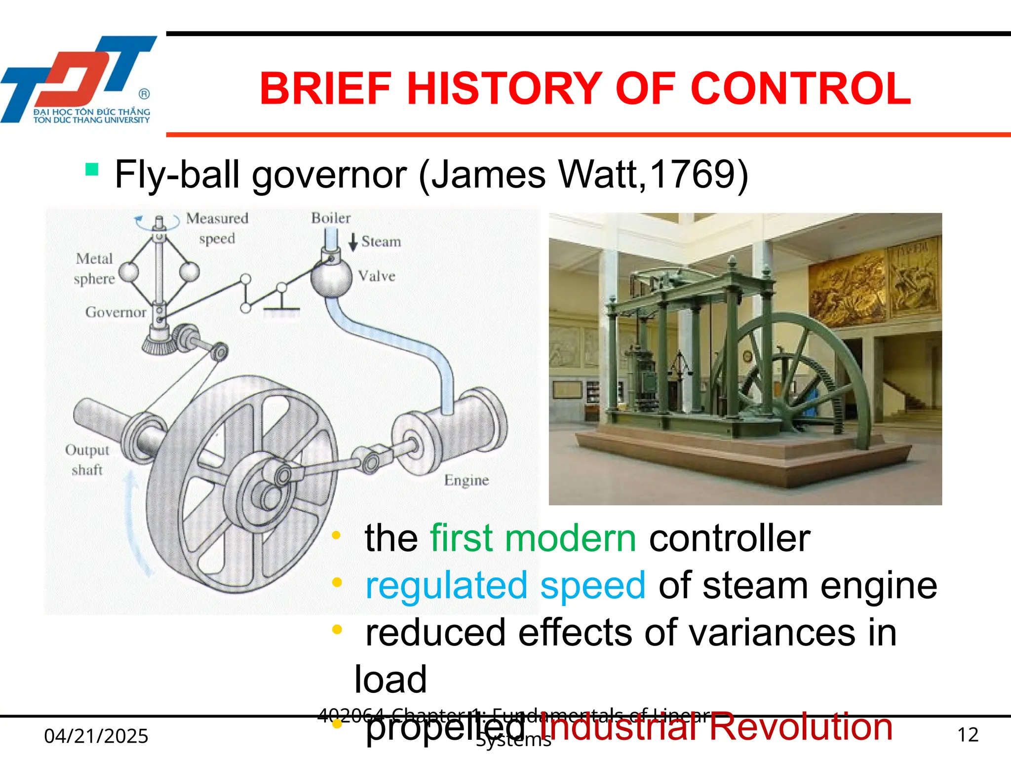
Fly-ball governor (James Watt,1769)
• the first modern controller
• regulated speed of steam engine
• reduced effects of variances in
load
• propelled Industrial Revolution
13.
CLASSIFICATION OF CONTROL
SYSTEMS
04/21/2025
402064-Chapter1: Fundamentals of Linear
Systems 13
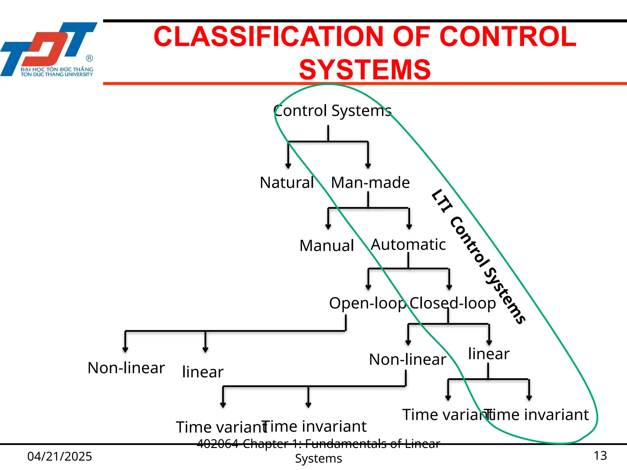
Control Systems
Natural Man-made
Manual Automatic
Open-loopClosed-loop
Non-linear linear
Time variant
Time invariant
Non-linear linear
Time variant
Time invariant L
T
I
C
o
n
t
r
o
l
S
y
s
t
e
m
s
14.
TYPES OF CONTROLSYSTEMS
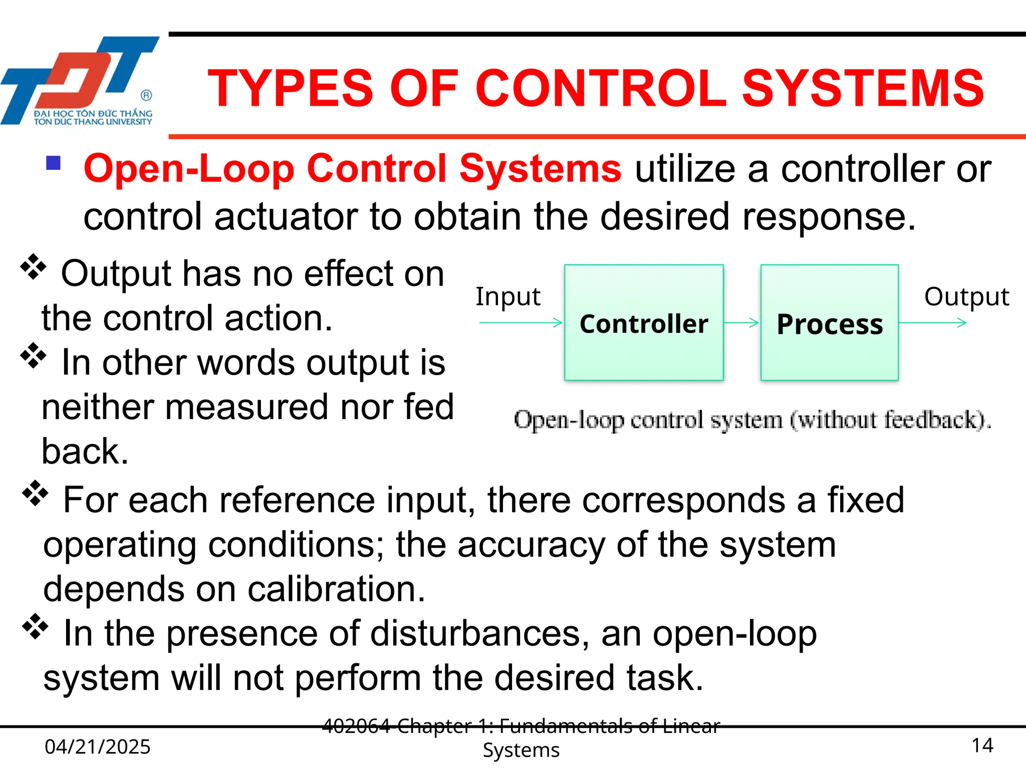
Open-Loop Control Systems utilize a controller or
control actuator to obtain the desired response.
04/21/2025
402064-Chapter 1: Fundamentals of Linear
Systems 14
Controller
Output
Input
Process
Output has no effect on
the control action.
In other words output is
neither measured nor fed
back.
For each reference input, there corresponds a fixed
operating conditions; the accuracy of the system
depends on calibration.
In the presence of disturbances, an open-loop
system will not perform the desired task.
15.
OPEN-LOOP CONTROL SYSTEMS
04/21/2025
402064-Chapter1: Fundamentals of Linear
Systems 15
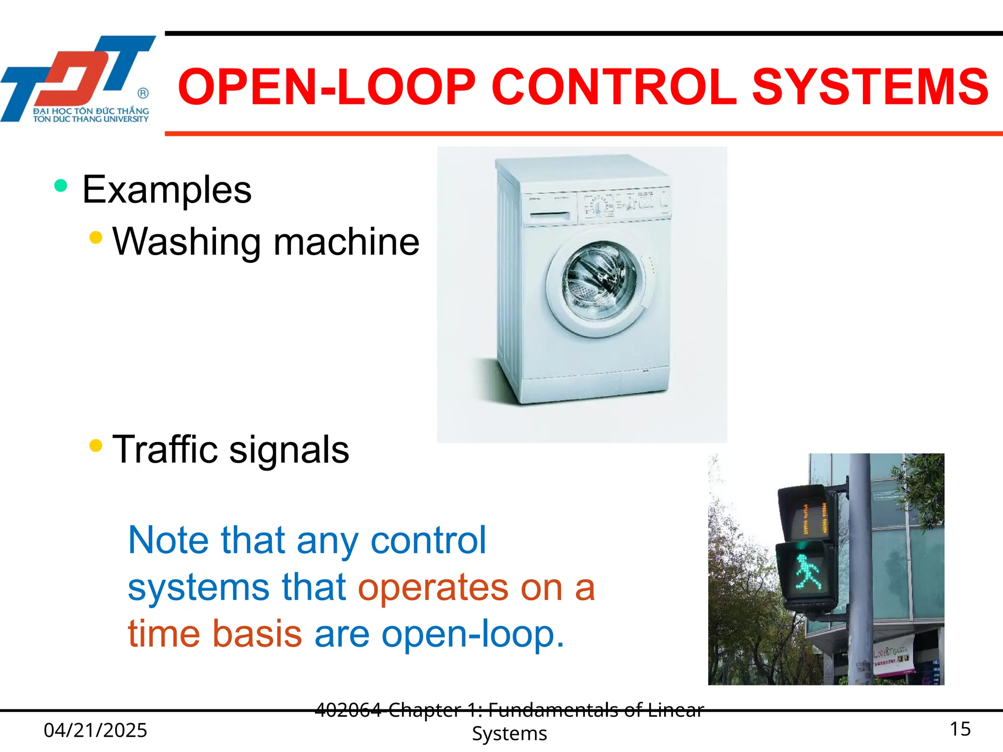
Examples
Washing machine
Traffic signals
Note that any control
systems that operates on a
time basis are open-loop.
16.
OPEN-LOOP CONTROL SYSTEMS
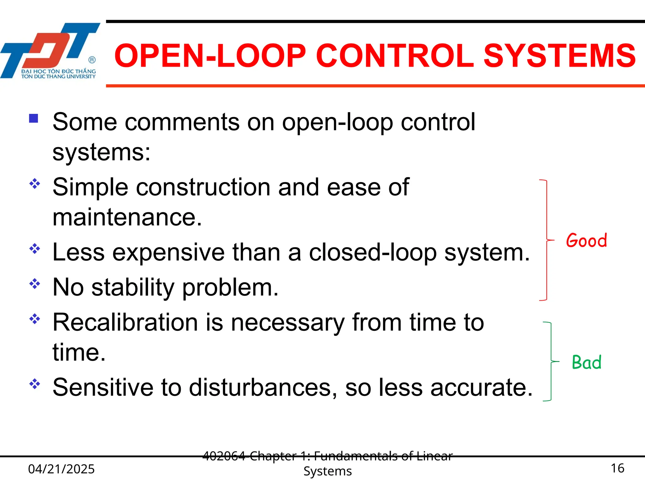
Some comments on open-loop control
systems:
Simple construction and ease of
maintenance.
Less expensive than a closed-loop system.
No stability problem.
Recalibration is necessary from time to
time.
Sensitive to disturbances, so less accurate.
04/21/2025
402064-Chapter 1: Fundamentals of Linear
Systems 16
Good
Bad
17.
TYPES OF CONTROLSYSTEMS
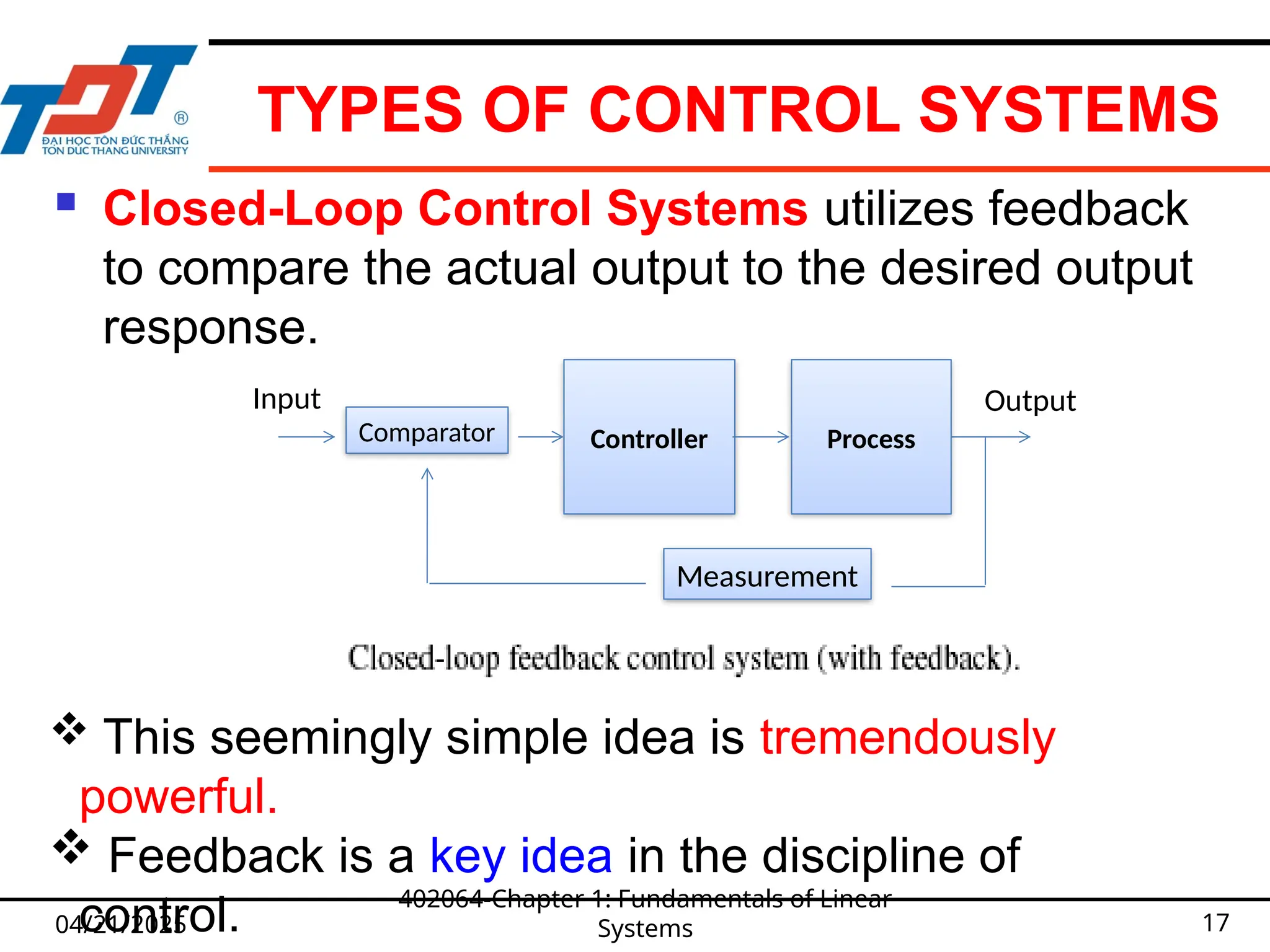
Closed-Loop Control Systems utilizes feedback
to compare the actual output to the desired output
response.
04/21/2025
402064-Chapter 1: Fundamentals of Linear
Systems 17
This seemingly simple idea is tremendously
powerful.
Feedback is a key idea in the discipline of
control.
Controller
Output
Input
Process
Comparator
Measurement
18.
CLOSED-LOOP CONTROL SYSTEMS
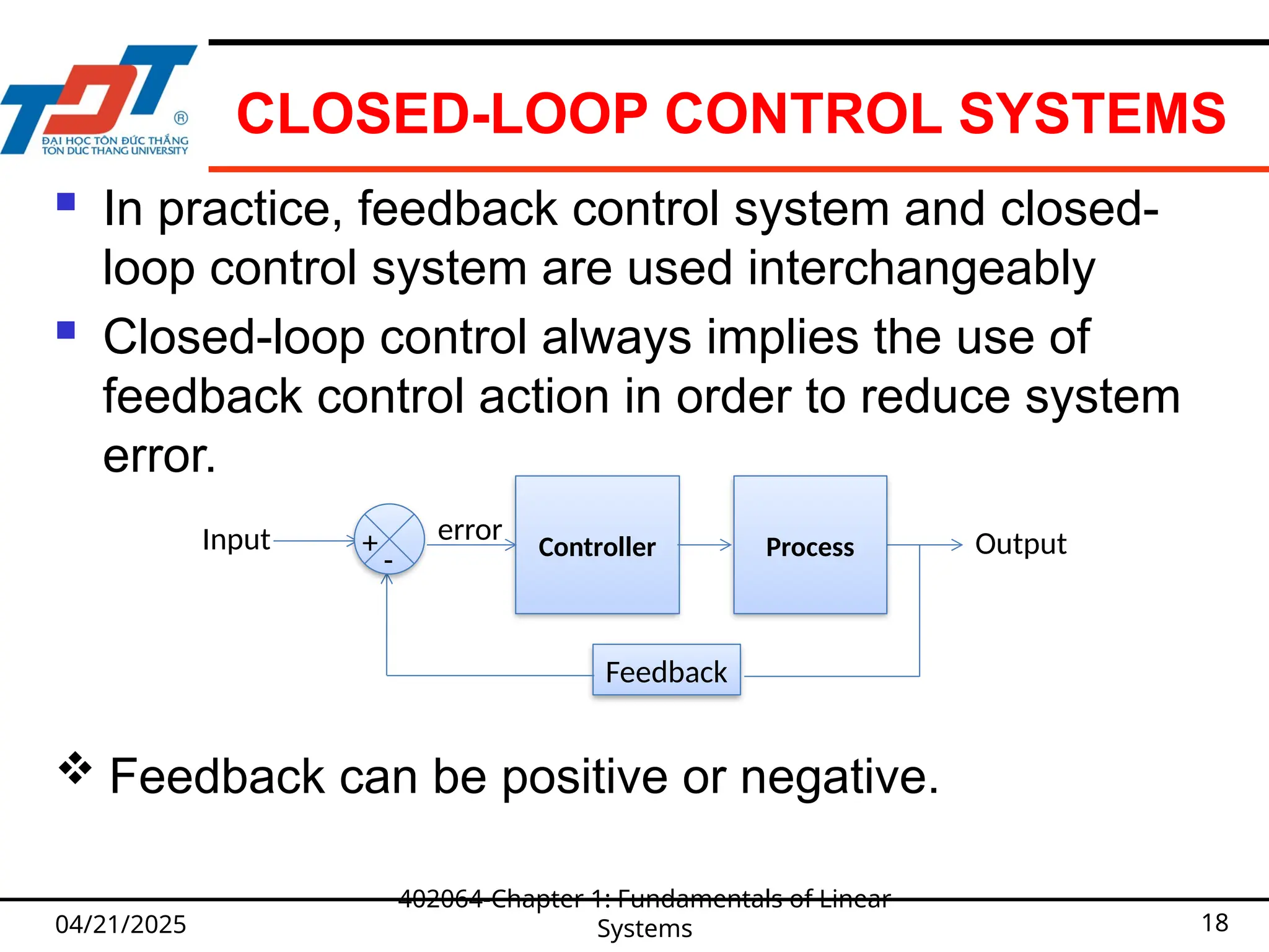
In practice, feedback control system and closed-
loop control system are used interchangeably
Closed-loop control always implies the use of
feedback control action in order to reduce system
error.
04/21/2025
402064-Chapter 1: Fundamentals of Linear
Systems 18
Feedback can be positive or negative.
Controller Output
Input Process
Feedback
-
+ error
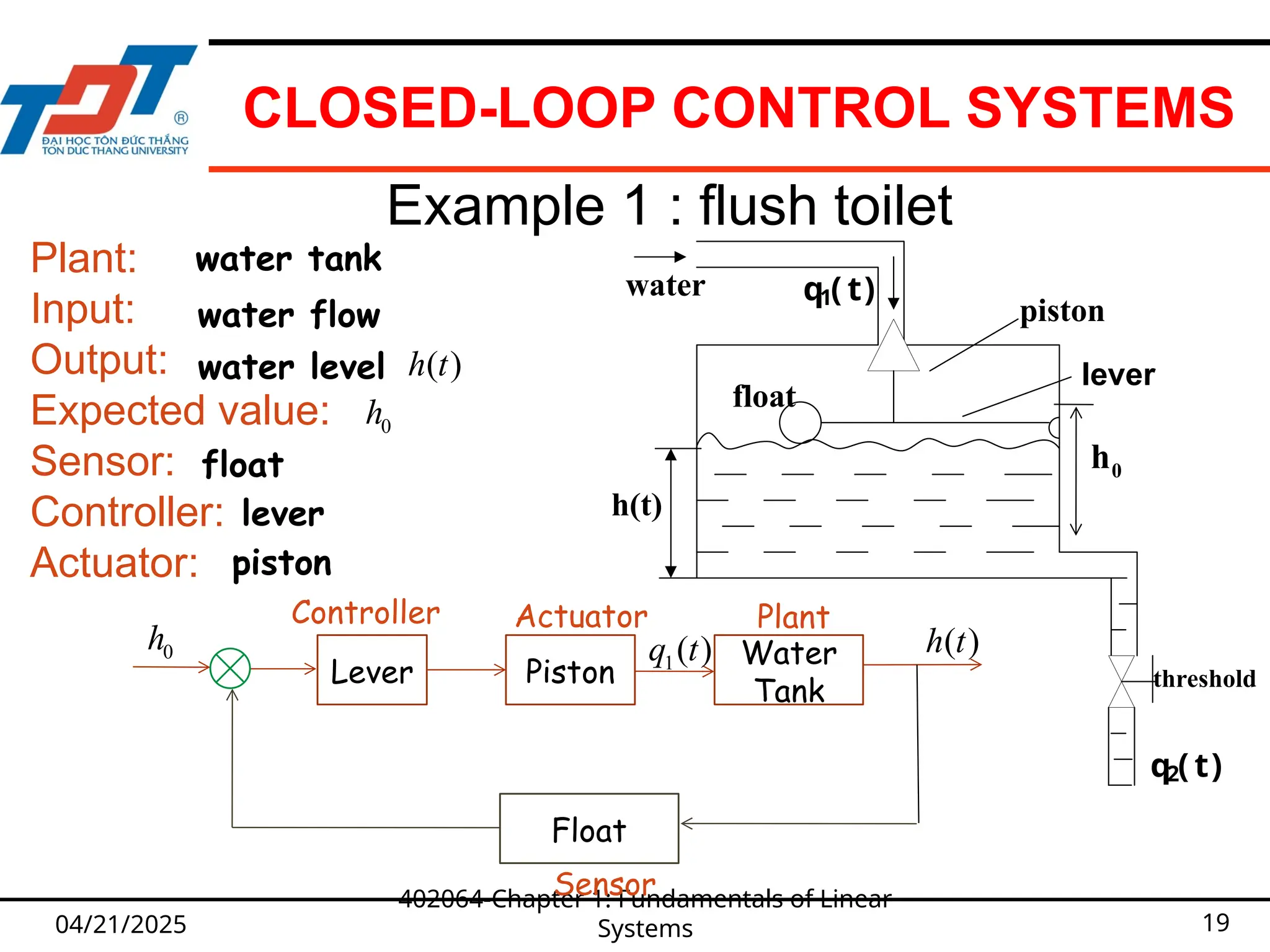
19.
CLOSED-LOOP CONTROL SYSTEMS
04/21/2025
402064-Chapter1: Fundamentals of Linear
Systems 19
Example 1 : flush toilet
threshold
piston
float
water
h(t)
q1( t)
q2( t)
Lever
Water
Tank
Float
Piston
0
h ( )
h t
1( )
q t
lever
Plant:
Input:
Output:
Expected value:
Sensor:
Controller:
Actuator:
0
h
( )
h t
0
h
Plant
Controller Actuator
Sensor
water tank
water flow
water level
float
lever
piston
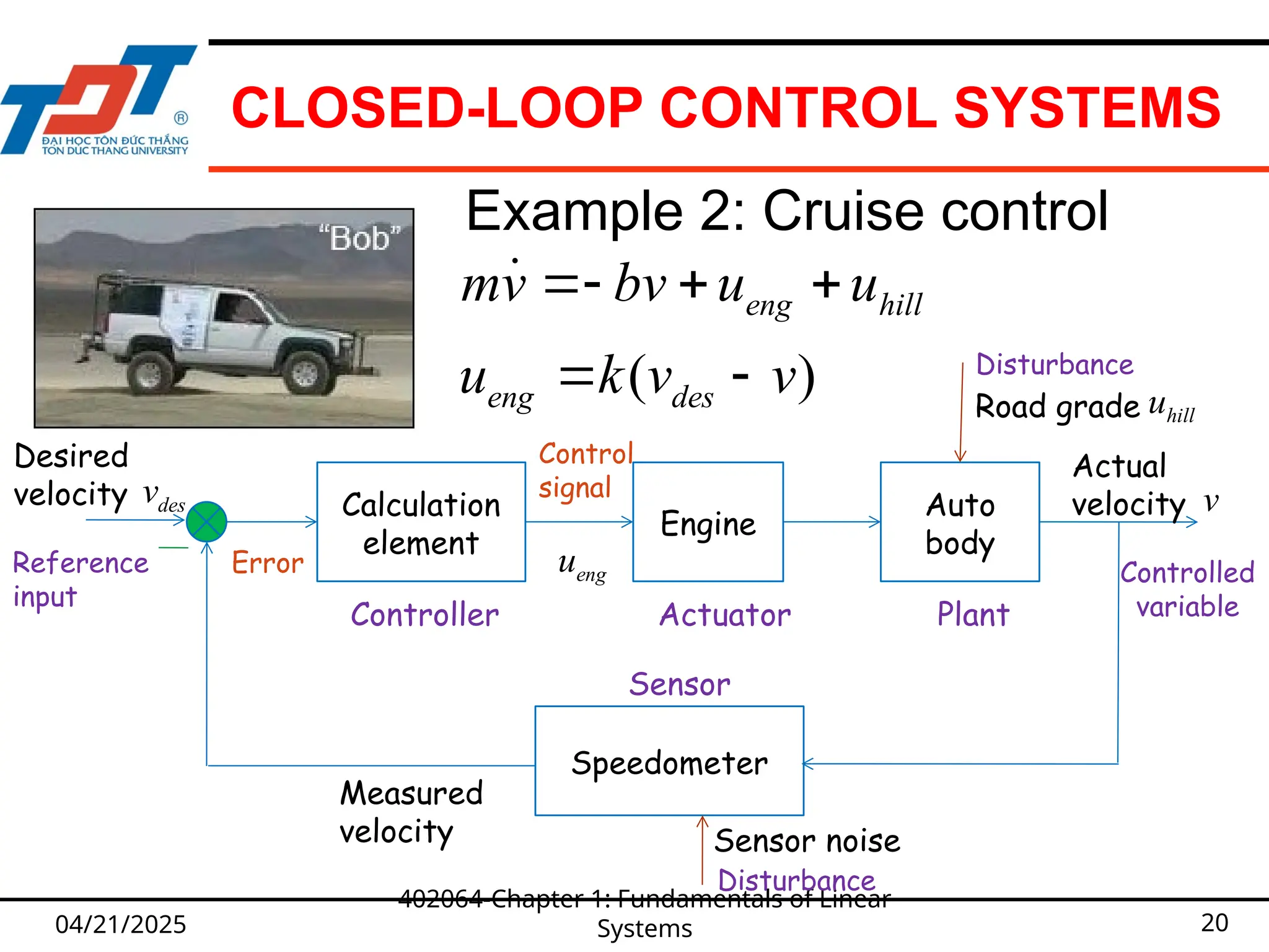
20.
CLOSED-LOOP CONTROL SYSTEMS
04/21/2025
402064-Chapter1: Fundamentals of Linear
Systems 20
Example 2: Cruise control
Calculation
element
Engine
Auto
body
Speedometer
Desired
velocity
Measured
velocity
Actual
velocity
Road grade
Sensor noise
Actuator
Controller Plant
Sensor
Controlled
variable
Reference
input
Disturbance
Disturbance
( )
eng hill
eng des
mv bv u u
u k v v
eng
u
hill
u
des
v v
Control
signal
Error
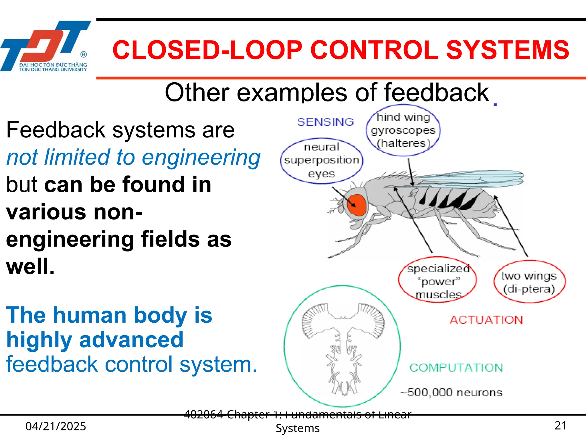
21.
CLOSED-LOOP CONTROL SYSTEMS
04/21/2025
402064-Chapter1: Fundamentals of Linear
Systems 21
Other examples of feedback
Feedback systems are
not limited to engineering
but can be found in
various non-
engineering fields as
well.
The human body is
highly advanced
feedback control system.
22.
CLOSED-LOOP CONTROL SYSTEMS
Main advantages of feedback:
Reduce disturbance effects, make system
insensitive to variations.
Stabilize an unstable system.
Create well-defined relationship between
output and reference.
04/21/2025
402064-Chapter 1: Fundamentals of Linear
Systems 22
23.
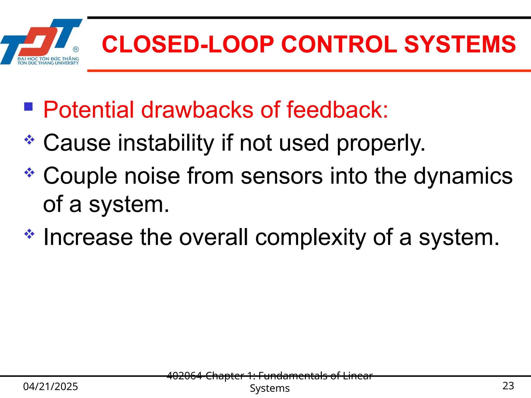
CLOSED-LOOP CONTROL SYSTEMS
Potential drawbacks of feedback:
Cause instability if not used properly.
Couple noise from sensors into the dynamics
of a system.
Increase the overall complexity of a system.
04/21/2025
402064-Chapter 1: Fundamentals of Linear
Systems 23
24.
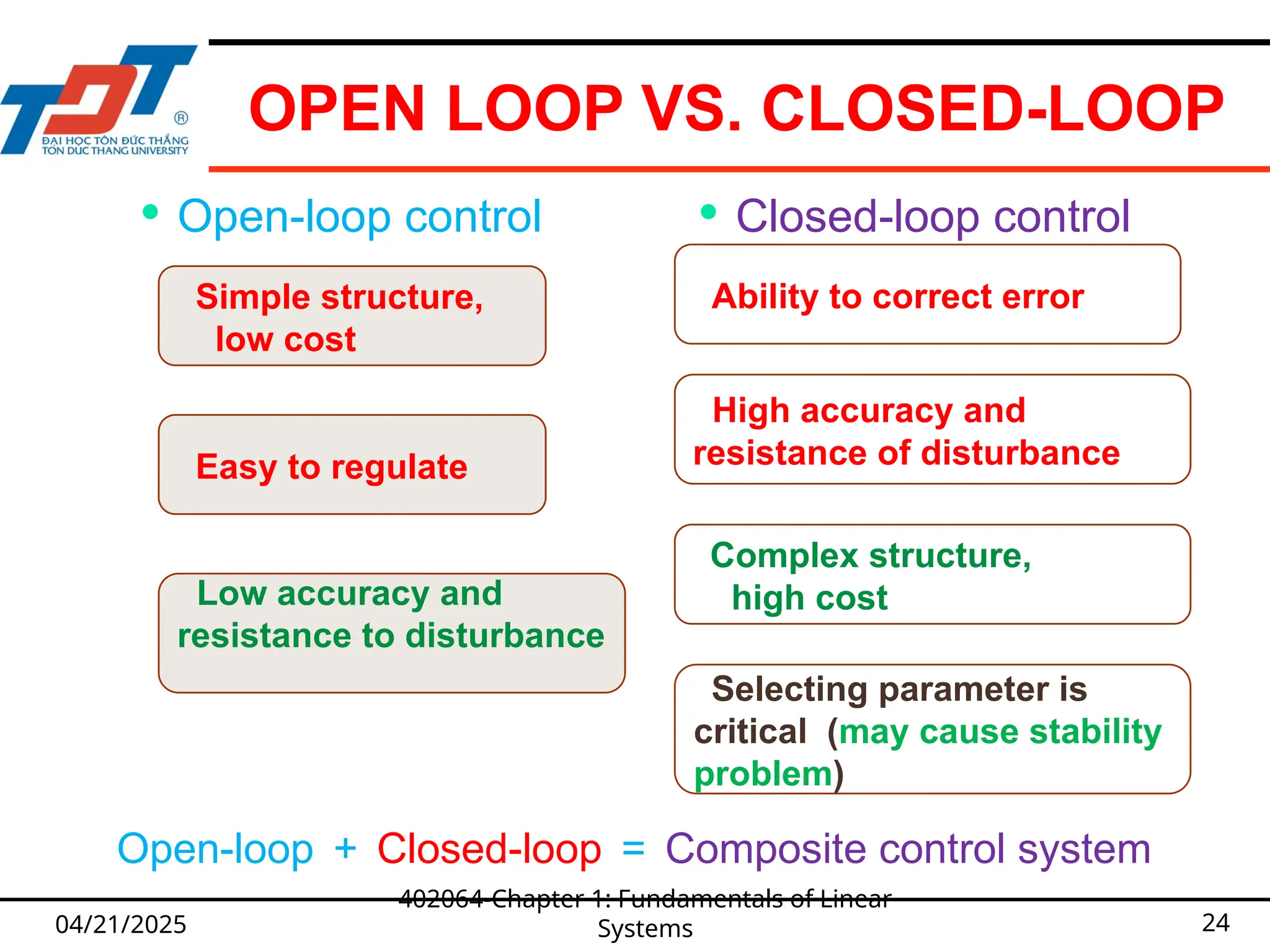
OPEN LOOP VS.CLOSED-LOOP
04/21/2025
402064-Chapter 1: Fundamentals of Linear
Systems 24
Open-loop control Closed-loop control
Simple structure,
low cost
Low accuracy and
resistance to disturbance
Easy to regulate
Ability to correct error
Complex structure,
high cost
High accuracy and
resistance of disturbance
Selecting parameter is
critical (may cause stability
problem)
Open-loop + Closed-loop = Composite control system
25.
THINKING TIME …
04/21/2025
402064-Chapter1: Fundamentals of Linear
Systems 25
Examples of open-loop
control and closed-loop
control systems ?
For each system, could
you identify the sensor,
actuator and controller?
26.
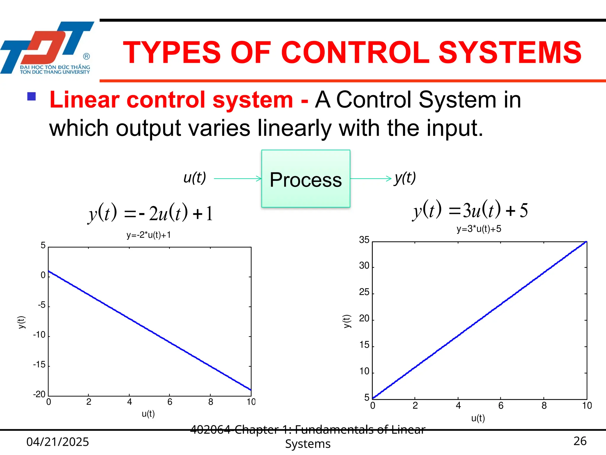
TYPES OF CONTROLSYSTEMS
Linear control system - A Control System in
which output varies linearly with the input.
04/21/2025
402064-Chapter 1: Fundamentals of Linear
Systems 26
5
3
)
(
)
( t
u
t
y
y(t)
u(t) Process
1
2
)
(
)
( t
u
t
y
0 2 4 6 8 10
5
10
15
20
25
30
35
y=3*u(t)+5
u(t)
y(t)
0 2 4 6 8 10
-20
-15
-10
-5
0
5
y(t)
u(t)
y=-2*u(t)+1
27.
TYPES OF CONTROLSYSTEMS
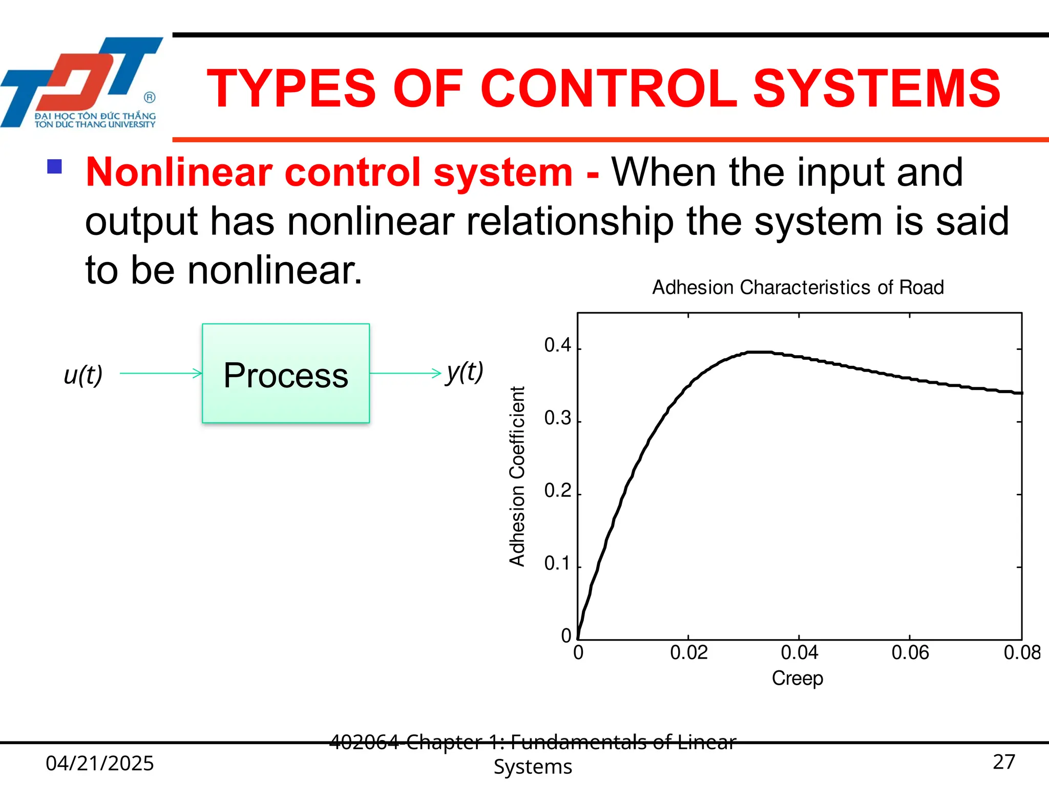
Nonlinear control system - When the input and
output has nonlinear relationship the system is said
to be nonlinear.
04/21/2025
402064-Chapter 1: Fundamentals of Linear
Systems 27
y(t)
u(t) Process
0 0.02 0.04 0.06 0.08
0
0.1
0.2
0.3
0.4
Adhesion Characteristics of Road
Creep
Adhesion
Coefficient
28.
TYPES OF CONTROLSYSTEMS
Quite often, nonlinear characteristics are
intentionally introduced in a control system to
improve its performance or provide more effective
control.
For instance, to achieve minimum-time control, an
on-off (bang-bang or relay) type controller is used in
many missile or spacecraft control systems.
There are no general methods for solving a wide
class of nonlinear systems.
Linear control systems are idealized models
fabricated by the analyst purely for the simplicity of
analysis and design.
04/21/2025
402064-Chapter 1: Fundamentals of Linear
Systems 28
29.
TYPES OF CONTROLSYSTEMS
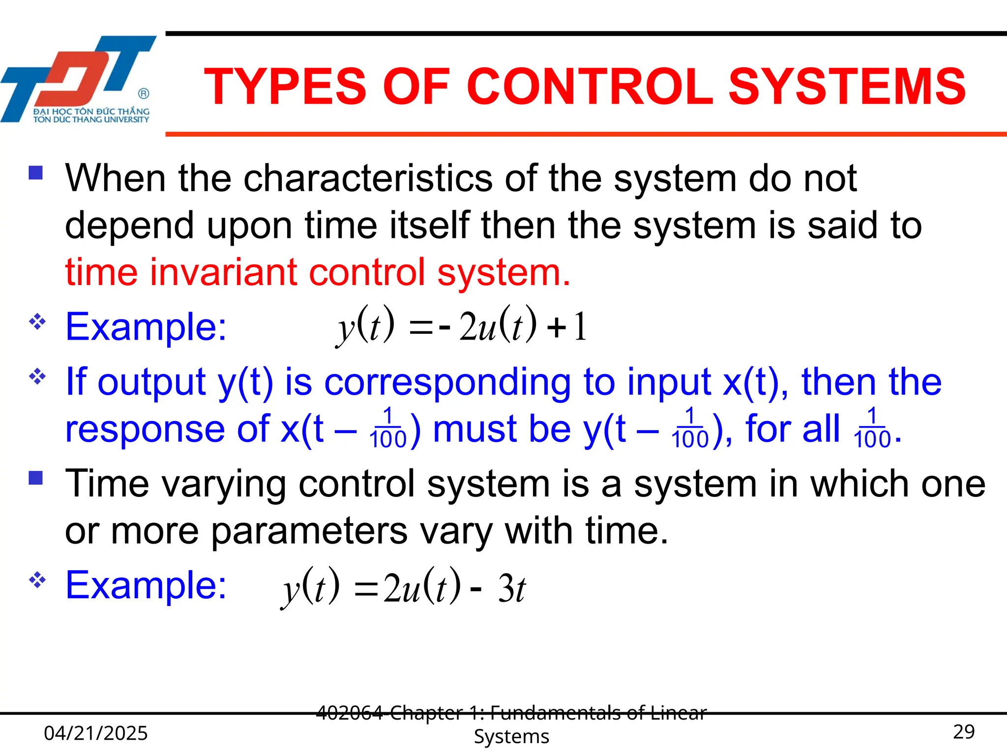
When the characteristics of the system do not
depend upon time itself then the system is said to
time invariant control system.
Example:
If output y(t) is corresponding to input x(t), then the
response of x(t – ) must be y(t – ), for all .
Time varying control system is a system in which one
or more parameters vary with time.
Example:
04/21/2025
402064-Chapter 1: Fundamentals of Linear
Systems 29
1
2
)
(
)
( t
u
t
y
t
t
u
t
y 3
2
)
(
)
(
30.
TYPES OF CONTROLSYSTEMS
In continuous data control system all system
variables are function of a continuous time t.
A discrete time control system involves one or more
variables that are known only at discrete time
intervals.
04/21/2025
402064-Chapter 1: Fundamentals of Linear
Systems 30
x(t)
t
X[n]
n
31.
TYPES OF CONTROLSYSTEMS
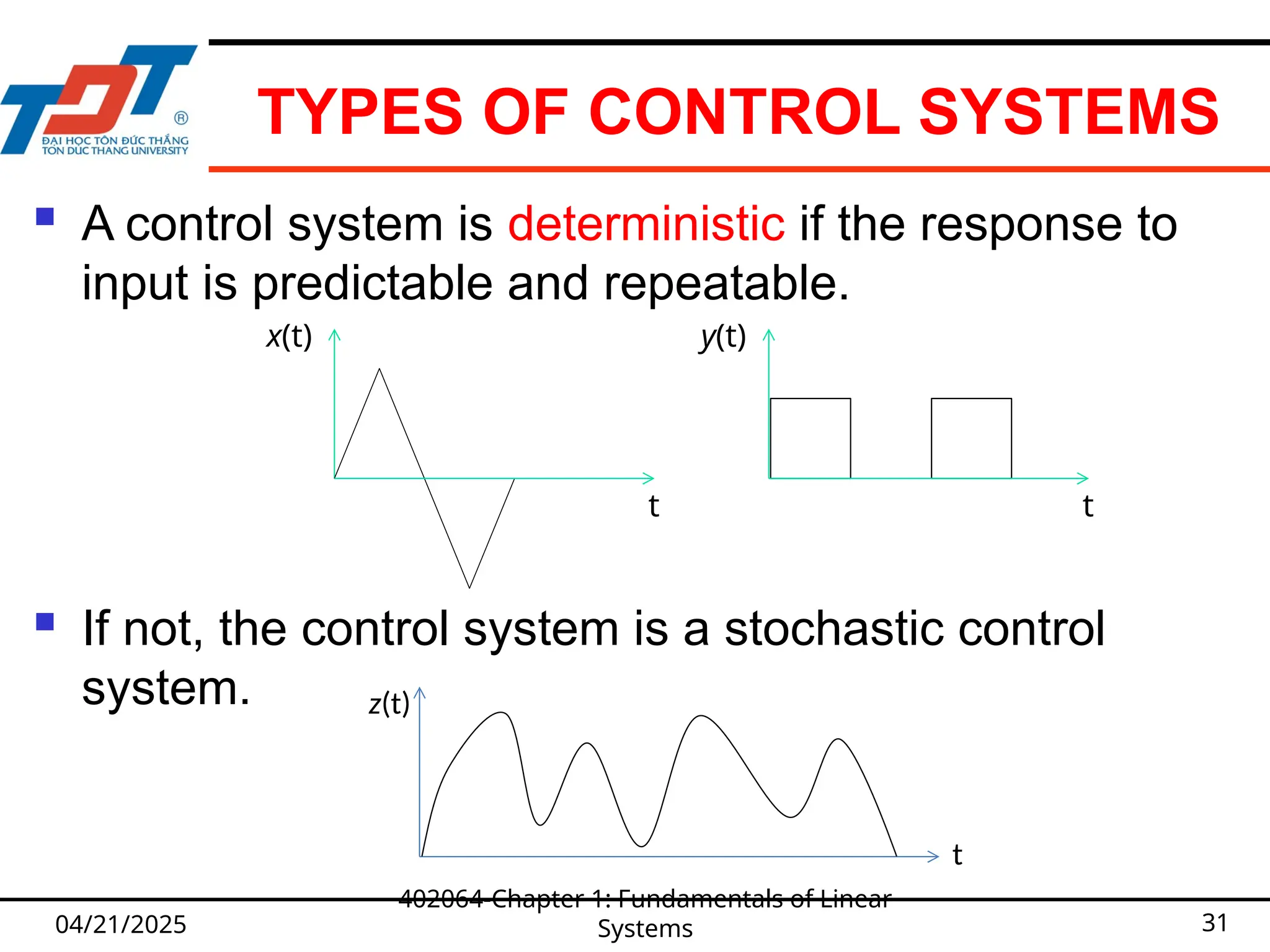
A control system is deterministic if the response to
input is predictable and repeatable.
If not, the control system is a stochastic control
system.
04/21/2025
402064-Chapter 1: Fundamentals of Linear
Systems 31
y(t)
t
x(t)
t
z(t)
t
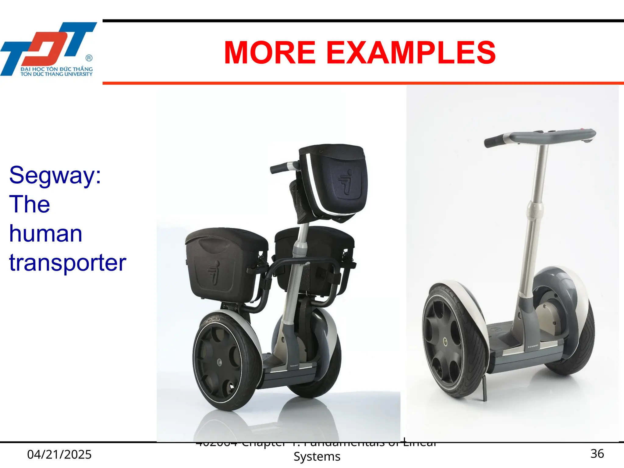
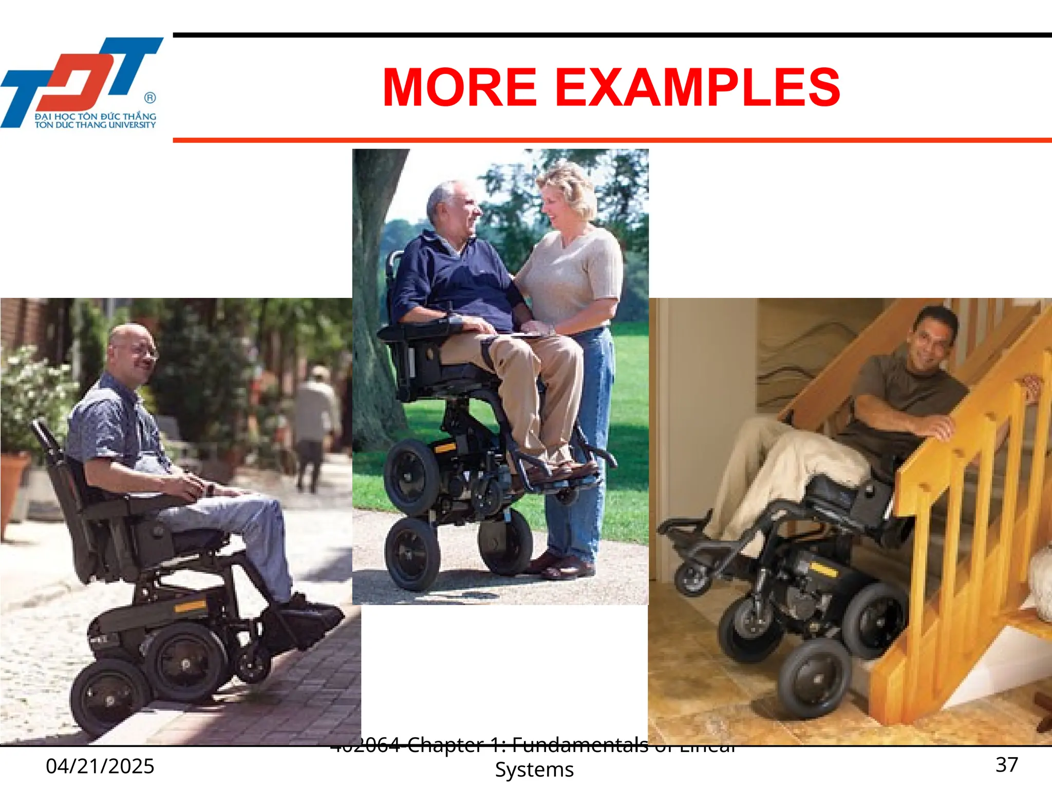
WHAT WE HAVELEARNT SO FAR?
So far we have learnt:
Concept of control systems
Classification of control systems
Assignment:
Read more examples in textbook.
Exercises: find more example of control
systems in real life.
04/21/2025
402064-Chapter 1: Fundamentals of Linear
Systems 38
39.
CHAPTER 1: FUNDAMENTALSOF
LINEAR SYSTEMS
1.1 Introduction
1.2 Linear algebra
1.3 Transfer function and impulse response
1.4 Representation of control systems
04/21/2025
402064-Chapter 1: Fundamentals of Linear
Systems 39
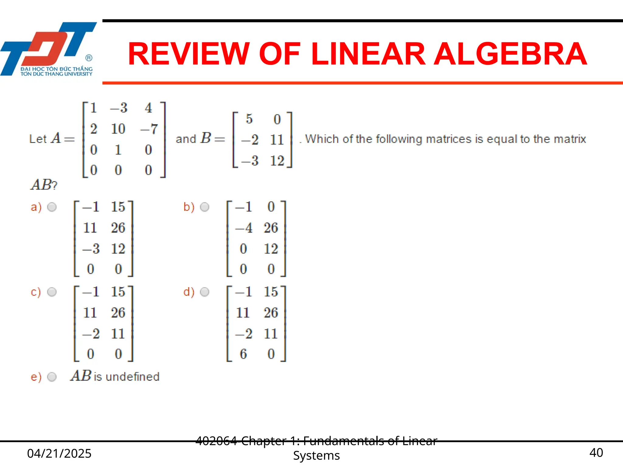
40.
REVIEW OF LINEARALGEBRA
04/21/2025
402064-Chapter 1: Fundamentals of Linear
Systems 40
41.
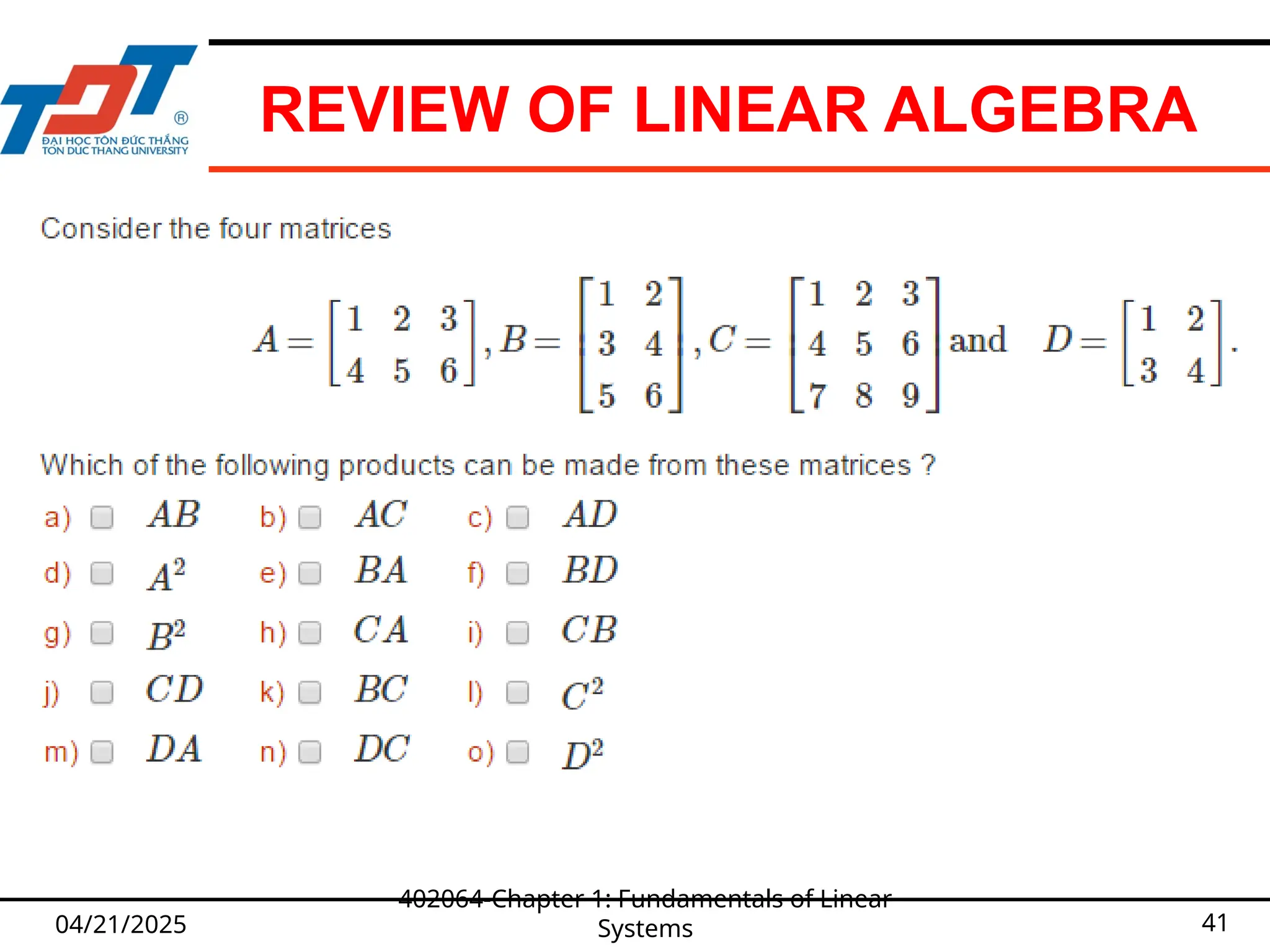
REVIEW OF LINEARALGEBRA
04/21/2025
402064-Chapter 1: Fundamentals of Linear
Systems 41
42.
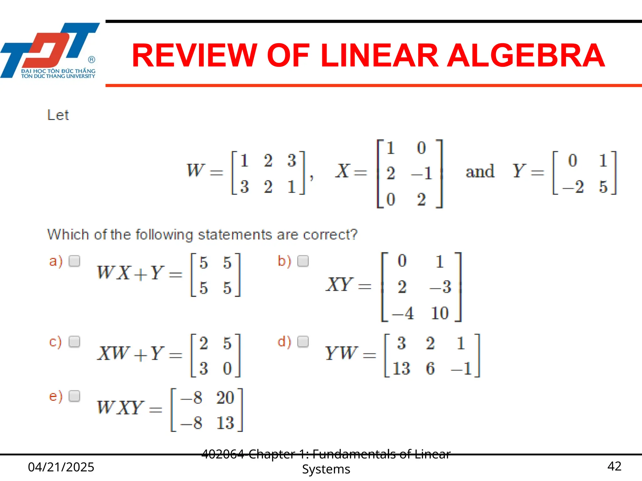
REVIEW OF LINEARALGEBRA
04/21/2025
402064-Chapter 1: Fundamentals of Linear
Systems 42
43.
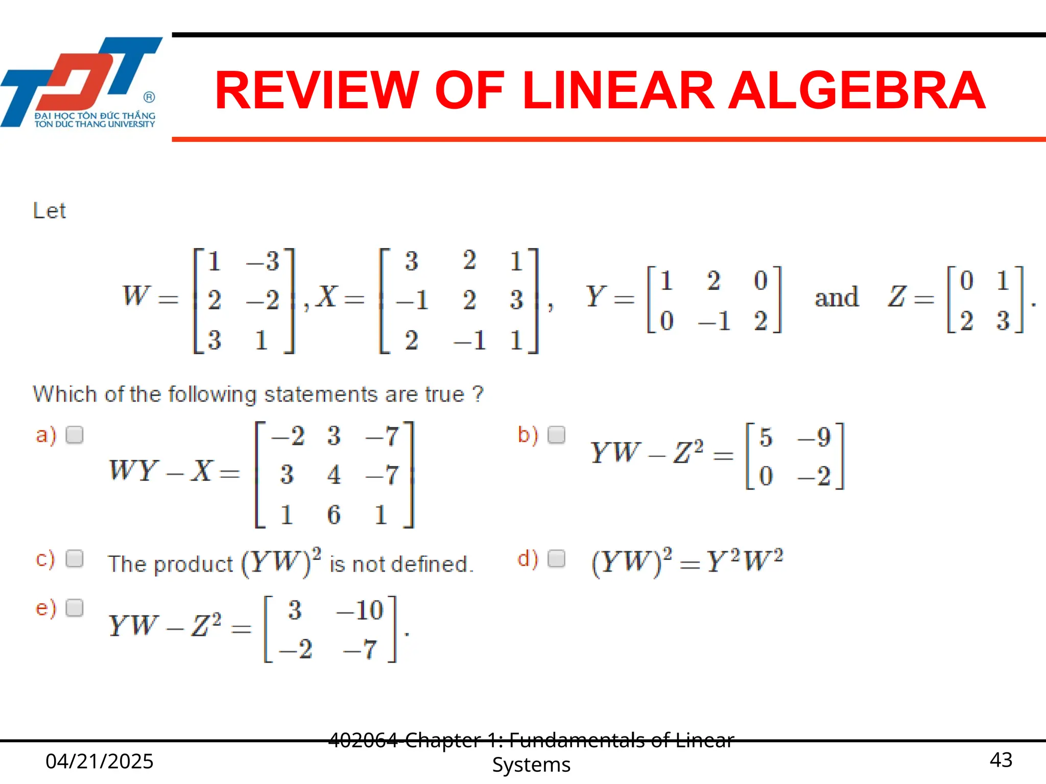
REVIEW OF LINEARALGEBRA
04/21/2025
402064-Chapter 1: Fundamentals of Linear
Systems 43
44.
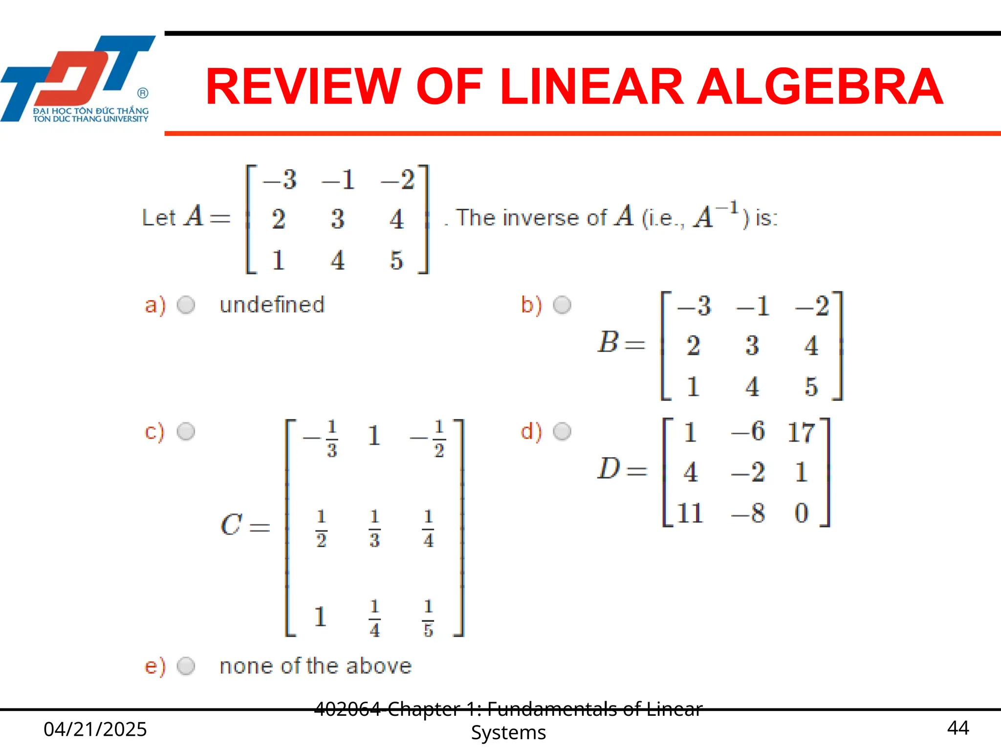
REVIEW OF LINEARALGEBRA
04/21/2025
402064-Chapter 1: Fundamentals of Linear
Systems 44
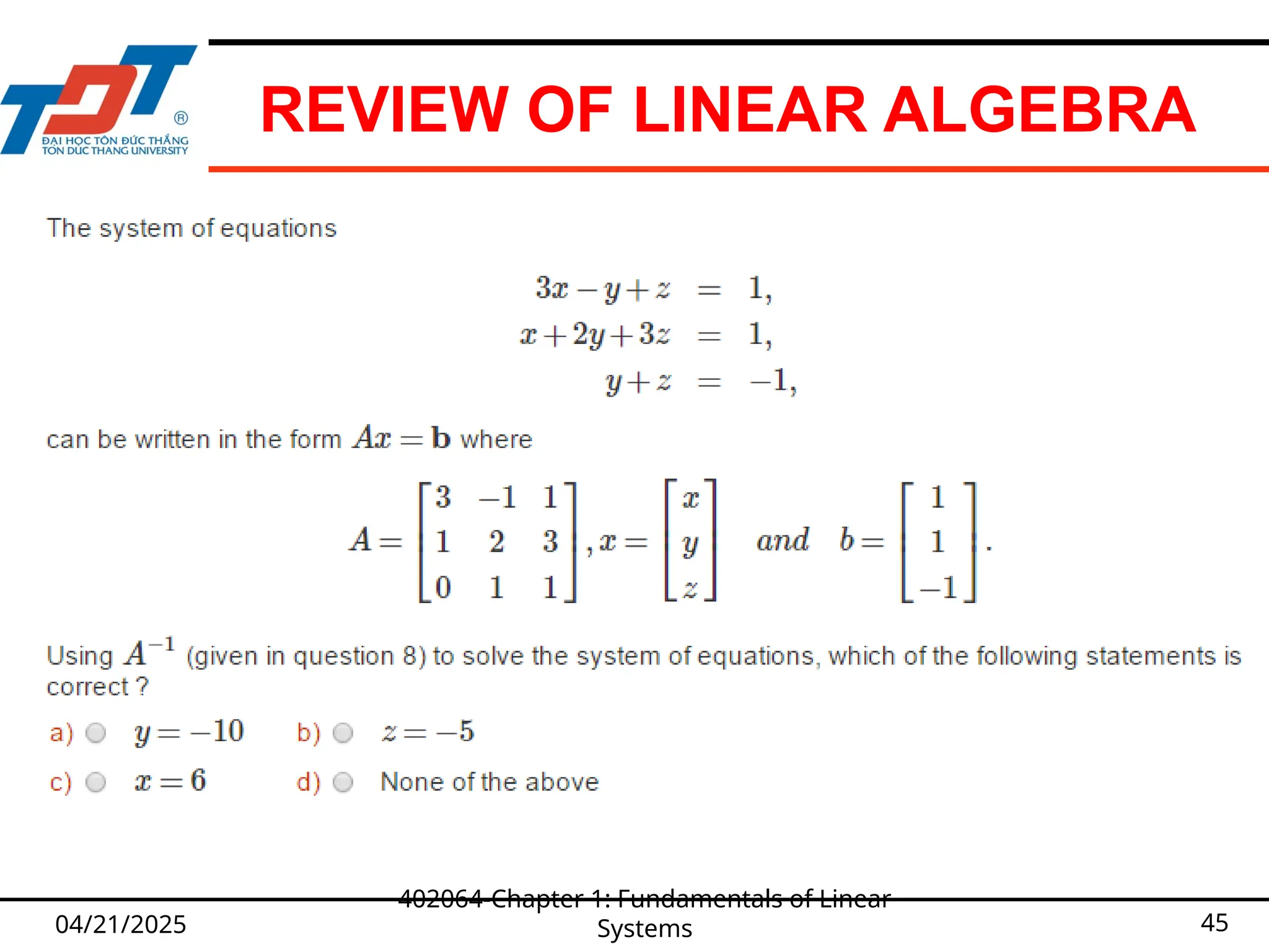
45.
REVIEW OF LINEARALGEBRA
04/21/2025
402064-Chapter 1: Fundamentals of Linear
Systems 45
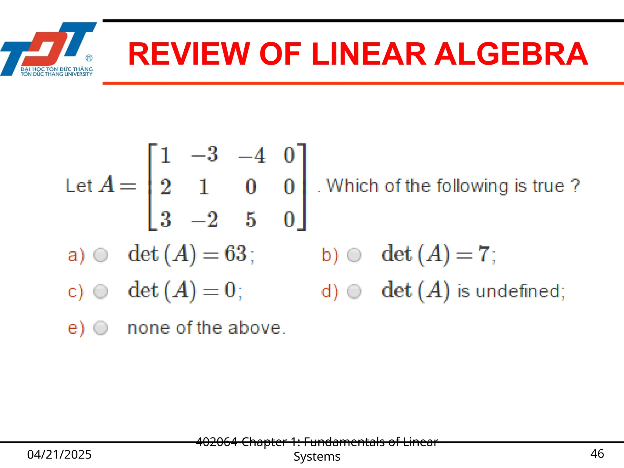
46.
REVIEW OF LINEARALGEBRA
04/21/2025
402064-Chapter 1: Fundamentals of Linear
Systems 46
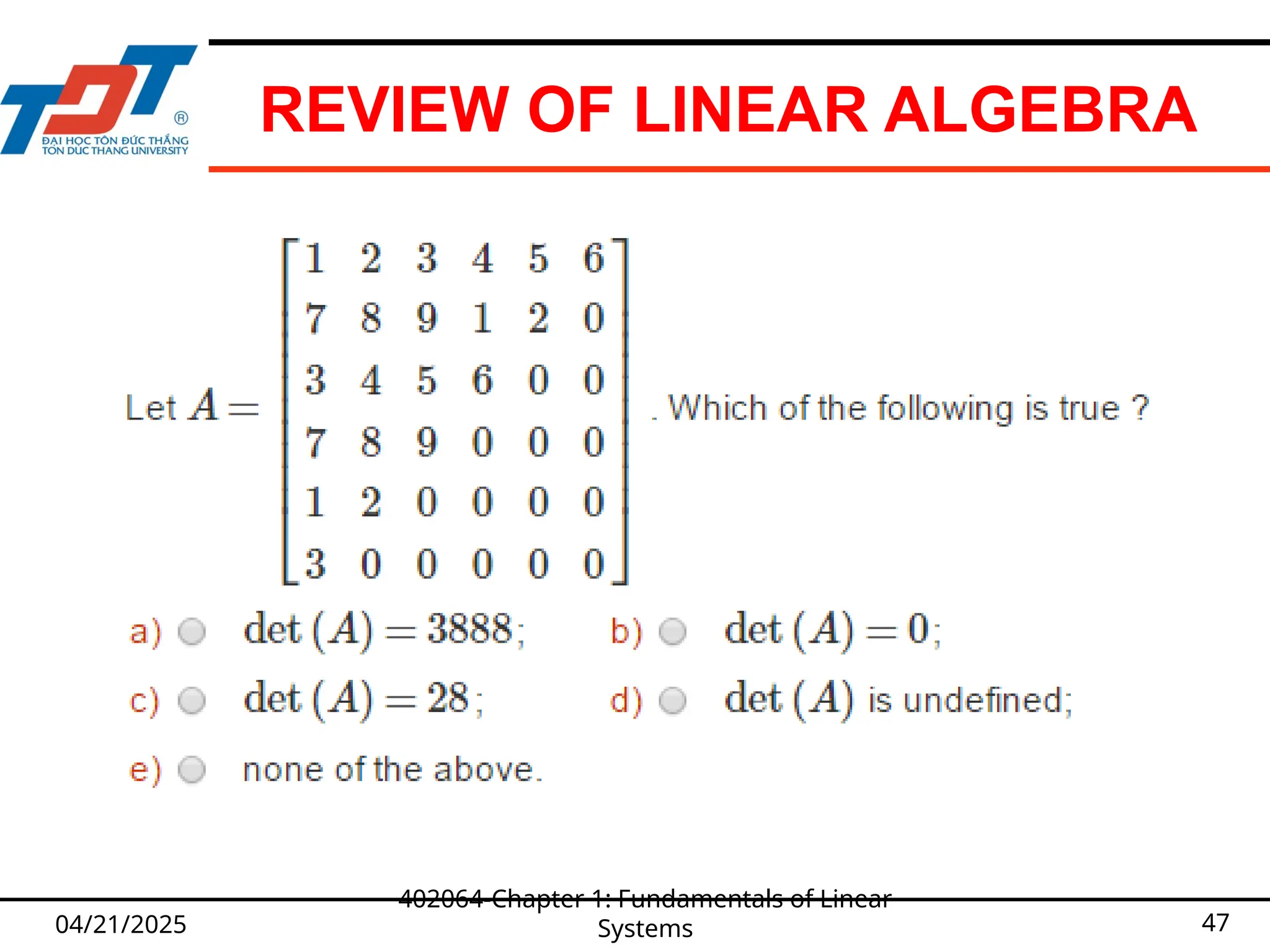
47.
REVIEW OF LINEARALGEBRA
04/21/2025
402064-Chapter 1: Fundamentals of Linear
Systems 47
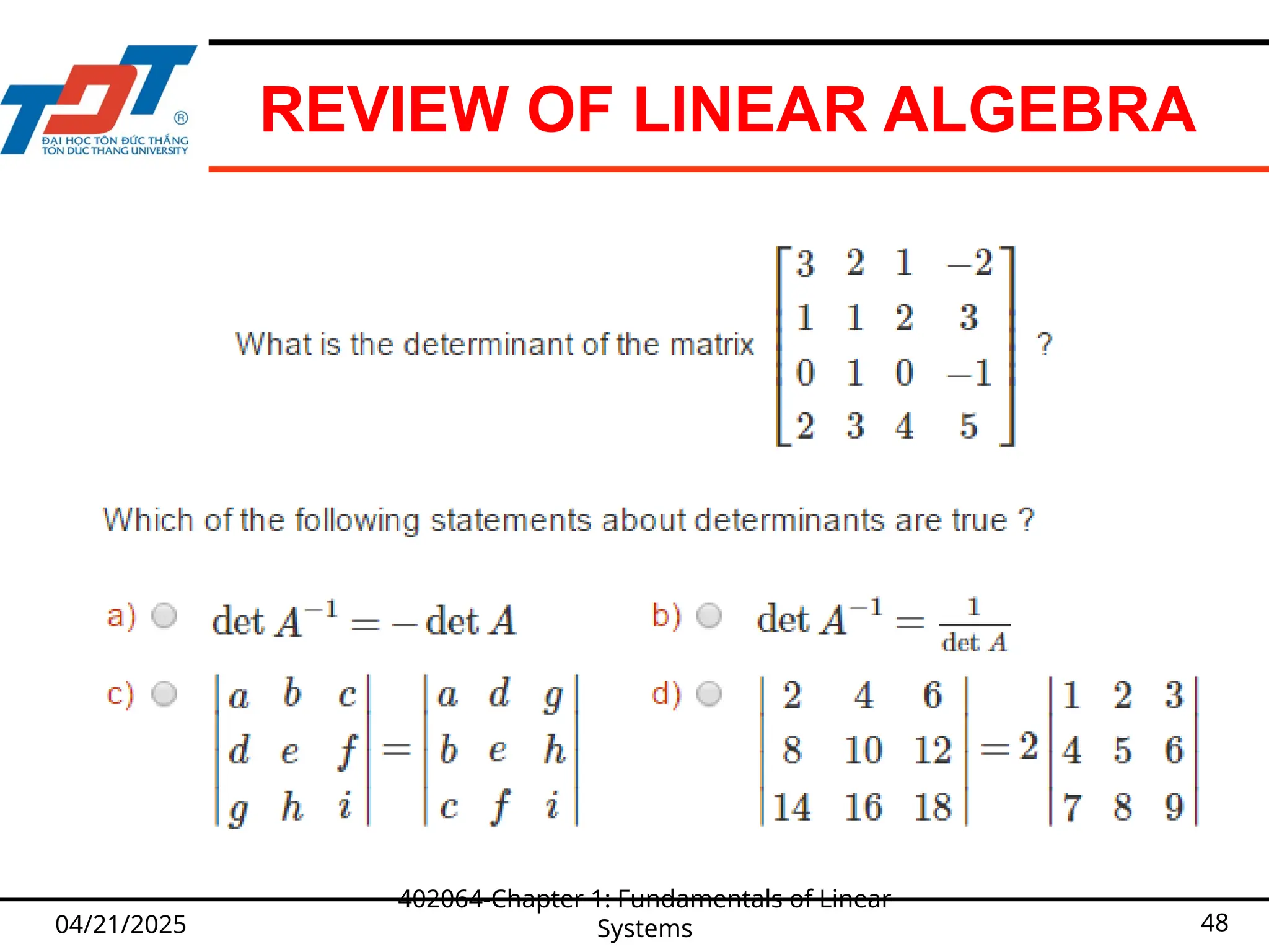
48.
REVIEW OF LINEARALGEBRA
04/21/2025
402064-Chapter 1: Fundamentals of Linear
Systems 48
49.
REVIEW OF LINEARALGEBRA
04/21/2025
402064-Chapter 1: Fundamentals of Linear
Systems 49
50.
REVIEW OF LINEARALGEBRA
04/21/2025
402064-Chapter 1: Fundamentals of Linear
Systems 50
51.
REVIEW OF LINEARALGEBRA
04/21/2025
402064-Chapter 1: Fundamentals of Linear
Systems 51
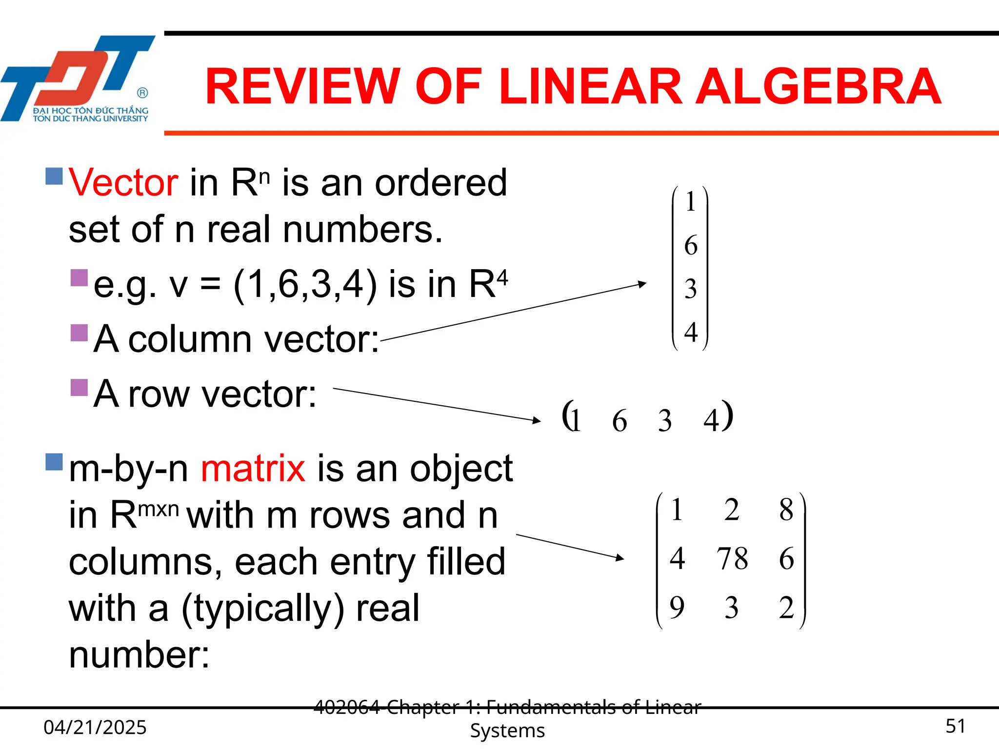
Vector in Rn
is an ordered
set of n real numbers.
e.g. v = (1,6,3,4) is in R4
A column vector:
A row vector:
m-by-n matrix is an object
in Rmxn
with m rows and n
columns, each entry filled
with a (typically) real
number:
4
3
6
1
4
3
6
1
2
3
9
6
78
4
8
2
1
52.
MATRICES
04/21/2025
402064-Chapter 1: Fundamentalsof Linear
Systems 52
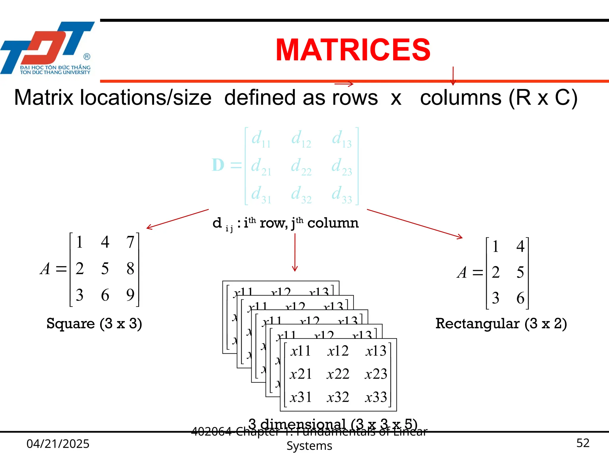
Square (3 x 3)
33
32
31
23
22
21
13
12
11
d
d
d
d
d
d
d
d
d
D
Matrix locations/size defined as rows x columns (R x C)
d i j : ith
row, jth
column
33
32
31
23
22
21
13
12
11
x
x
x
x
x
x
x
x
x
Rectangular (3 x 2)
33
32
31
23
22
21
13
12
11
x
x
x
x
x
x
x
x
x
33
32
31
23
22
21
13
12
11
x
x
x
x
x
x
x
x
x
33
32
31
23
22
21
13
12
11
x
x
x
x
x
x
x
x
x
33
32
31
23
22
21
13
12
11
x
x
x
x
x
x
x
x
x
9
6
3
8
5
2
7
4
1
A
6
5
4
3
2
1
A
3 dimensional (3 x 3 x 5)
53.
MATRIX CALCULUS
04/21/2025
402064-Chapter 1:Fundamentals of Linear
Systems 53
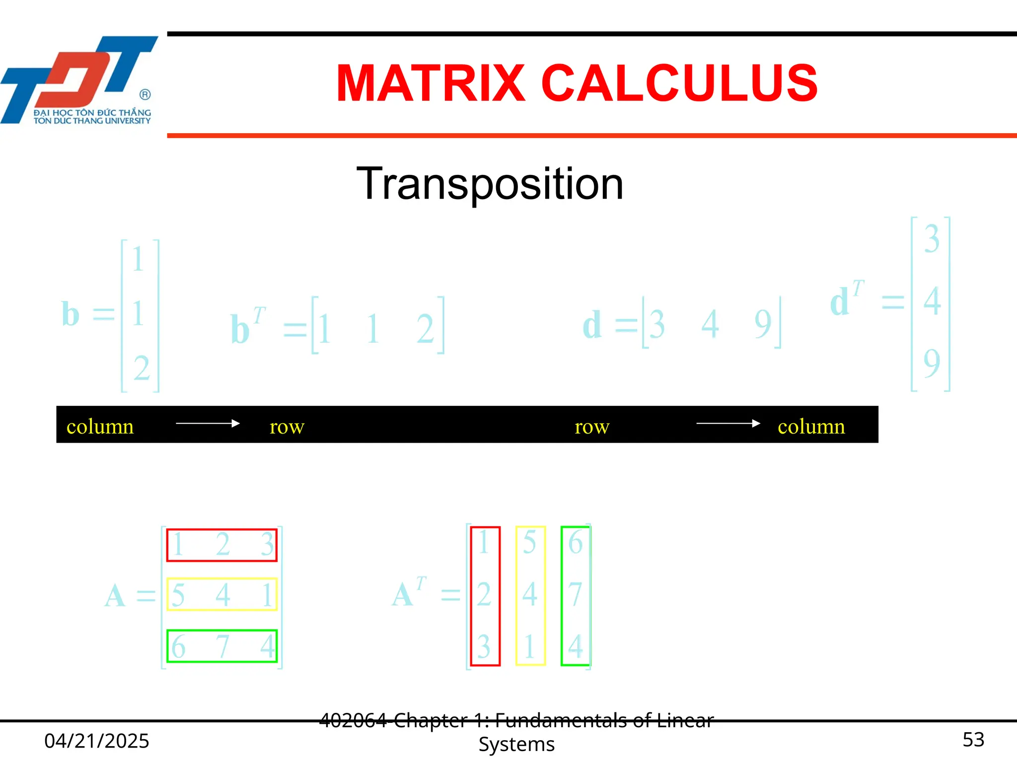
Transposition
column row row column
9
4
3
T
d
4
7
6
1
4
5
3
2
1
A
4
1
3
7
4
2
6
5
1
T
A
2
1
1
b
2
1
1
T
b
9
4
3
d
04/21/2025
402064-Chapter 1: Fundamentalsof Linear
Systems 55
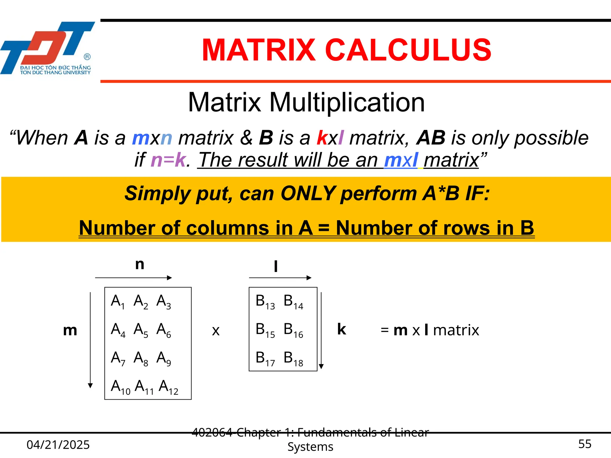
Matrix Multiplication
“When A is a mxn matrix & B is a kxl matrix, AB is only possible
if n=k. The result will be an mxl matrix”
A1 A2 A3
A4 A5 A6
A7 A8 A9
A10 A11 A12
m
n
x
B13 B14
B15 B16
B17 B18
l
k
Simply put, can ONLY perform A*B IF:
Number of columns in A = Number of rows in B
= m x l matrix
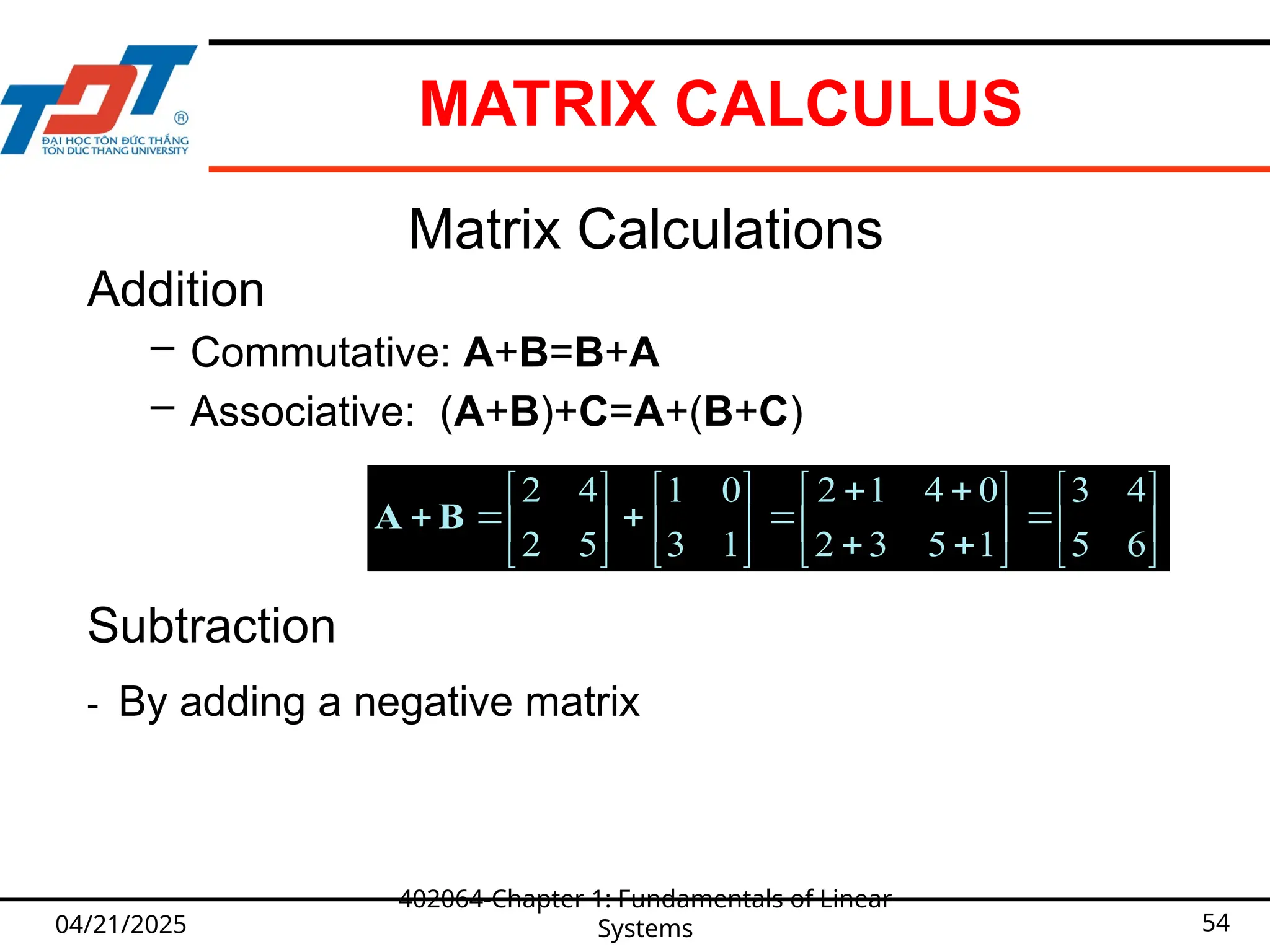
MATRIX CALCULUS
56.
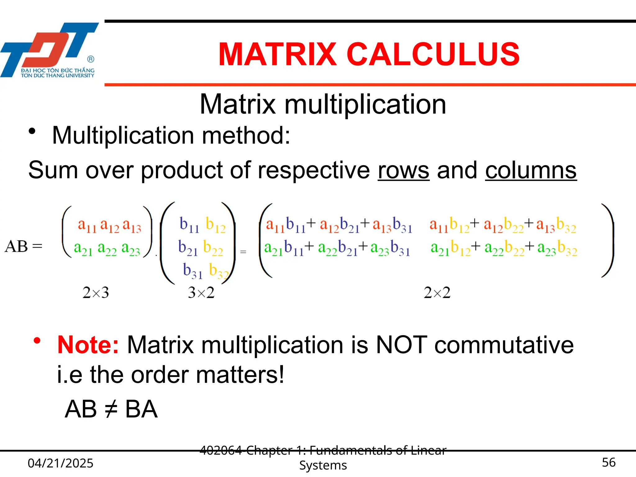
MATRIX CALCULUS
04/21/2025
402064-Chapter 1:Fundamentals of Linear
Systems 56
Matrix multiplication
• Multiplication method:
Sum over product of respective rows and columns
• Note: Matrix multiplication is NOT commutative
i.e the order matters!
AB ≠ BA
57.
04/21/2025
402064-Chapter 1: Fundamentalsof Linear
Systems 57
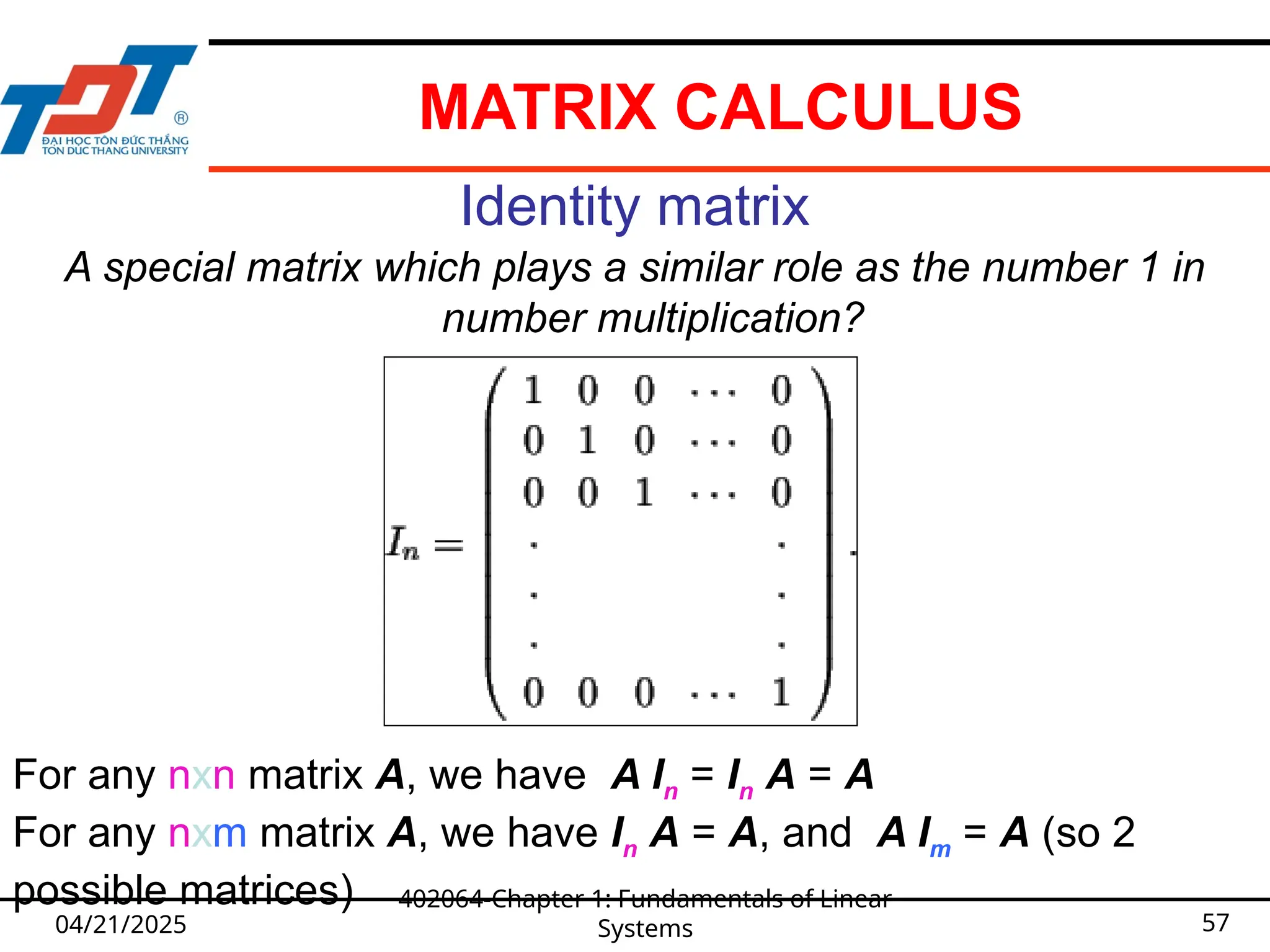
Identity matrix
A special matrix which plays a similar role as the number 1 in
number multiplication?
For any nxn matrix A, we have A In = In A = A
For any nxm matrix A, we have In A = A, and A Im = A (so 2
possible matrices)
MATRIX CALCULUS
58.
VECTOR NORM ANDDOT PRODUCT
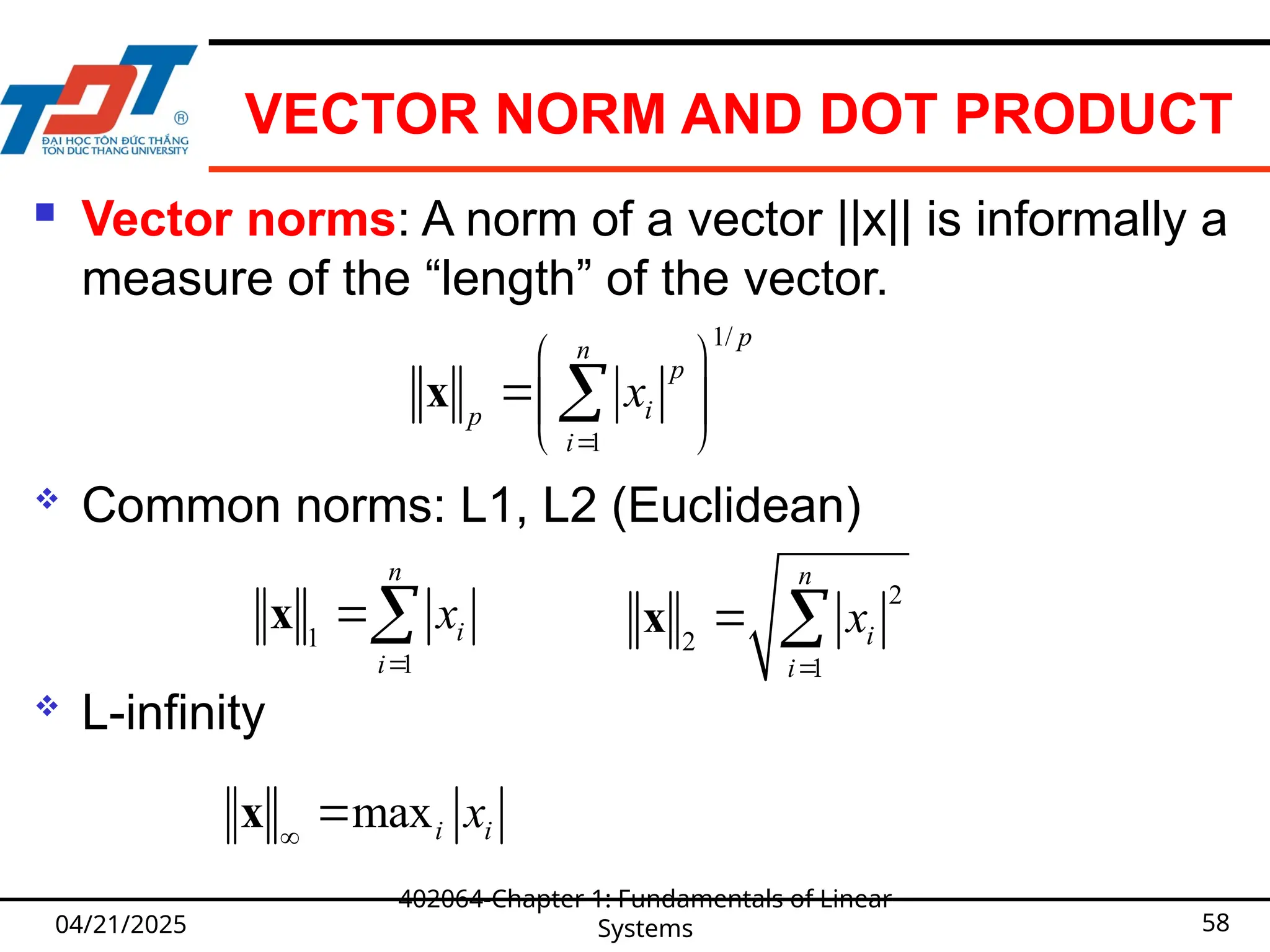
Vector norms: A norm of a vector ||x|| is informally a
measure of the “length” of the vector.
Common norms: L1, L2 (Euclidean)
L-infinity
04/21/2025
402064-Chapter 1: Fundamentals of Linear
Systems 58
1/
1
p
n
p
i
p
i
x
x
1
1
n
i
i
x
x
2
2
1
n
i
i
x
x
maxi i
x
x
59.
VECTOR NORM ANDDOT PRODUCT
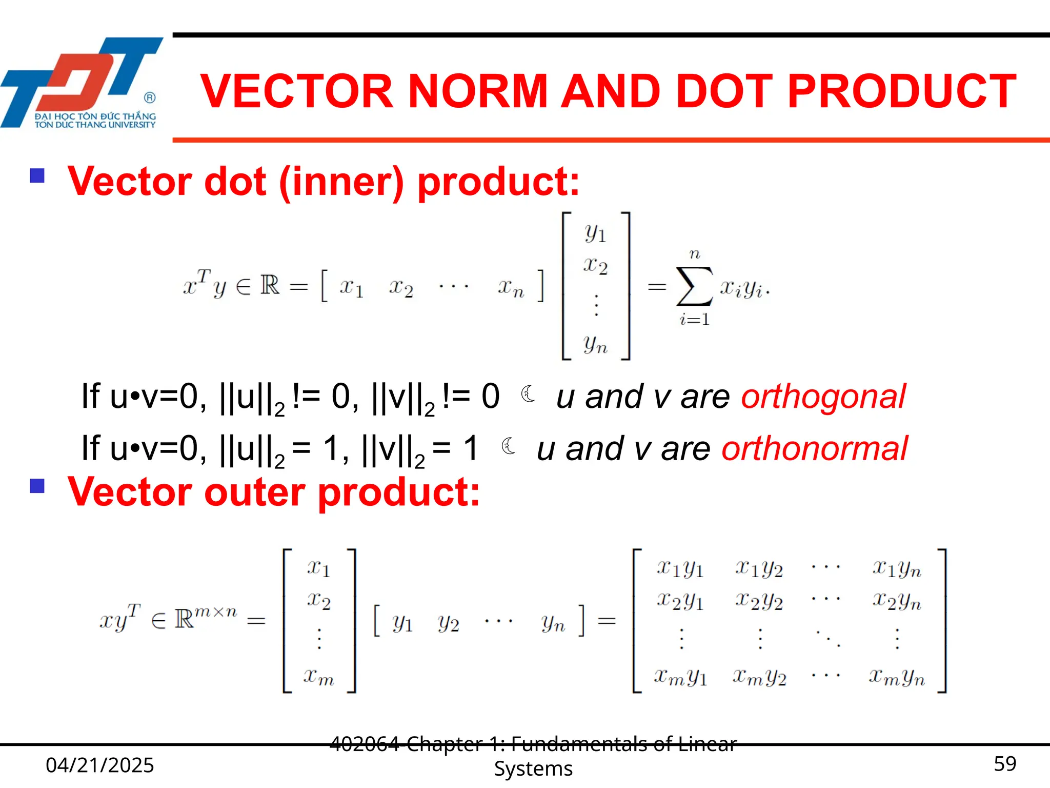
Vector dot (inner) product:
Vector outer product:
04/21/2025
402064-Chapter 1: Fundamentals of Linear
Systems 59
If u•v=0, ||u||2 != 0, ||v||2 != 0 u and v are orthogonal
If u•v=0, ||u||2 = 1, ||v||2 = 1 u and v are orthonormal
60.
LINEAR COMBINATION &VECTOR
SPACE
A linear combination of vectors is a vector that
can be obtained by multiplying these vectors by a
real number then adding them.
The vector space defined by some vectors is a
space that contains all linear combinations of them.
A matrix A (m x n) can itself be decomposed in as
many vectors as its number of columns (or rows).
Each column of the matrix can be represented as a
vector. The ensemble of n vector-column defines a
vector space proper to matrix A.
04/21/2025
402064-Chapter 1: Fundamentals of Linear
Systems 60
61.
LINEAR INDEPENDENCE
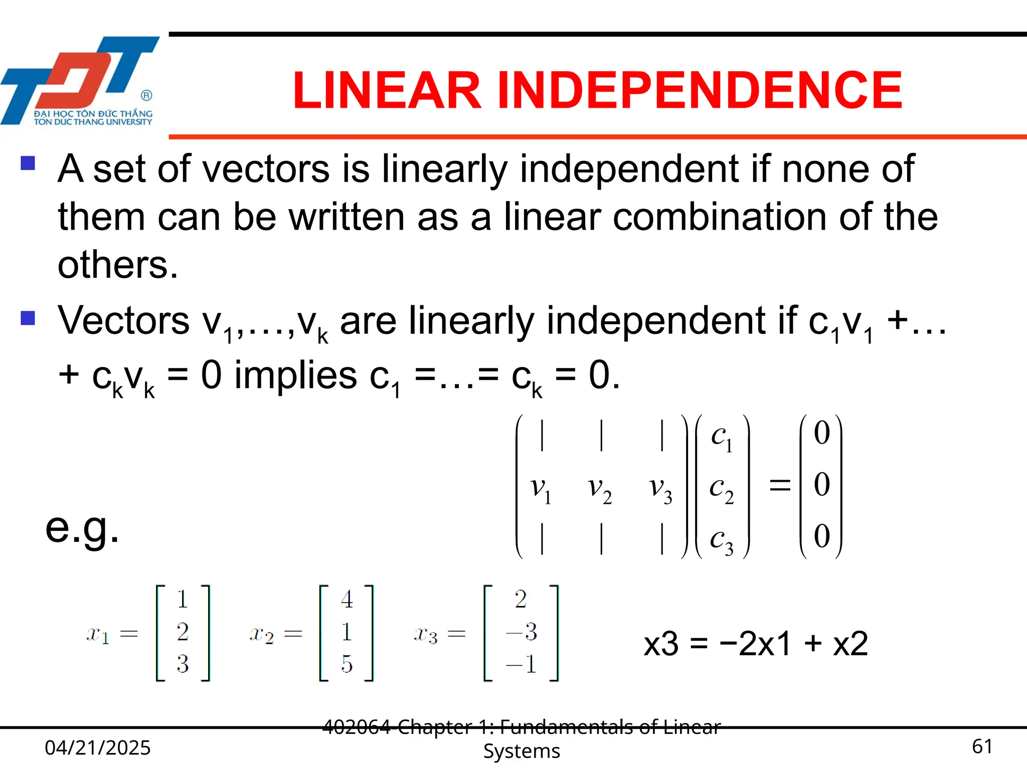
Aset of vectors is linearly independent if none of
them can be written as a linear combination of the
others.
Vectors v1,…,vk are linearly independent if c1v1 +…
+ ckvk = 0 implies c1 =…= ck = 0.
04/21/2025
402064-Chapter 1: Fundamentals of Linear
Systems 61
0
0
0
|
|
|
|
|
|
3
2
1
3
2
1
c
c
c
v
v
v
e.g.
x3 = −2x1 + x2
62.
DIMENSION & BASISOF A VECTOR
SPACE
If all vectors in a vector space may be expressed
as linear combinations of a set of vectors v1,…,vk,
then v1,…,vk spans the space.
A basis is a maximal set of linearly independent
vectors and a minimal set of spanning vectors of a
vector space.
The cardinality of a basis is the dimension of the
vector space.
A basis is a maximal set of linearly independent
vectors and a minimal set of spanning vectors of a
vector space.
04/21/2025
402064-Chapter 1: Fundamentals of Linear
Systems 62
63.
DIMENSION & BASISOF A VECTOR
SPACE
04/21/2025
402064-Chapter 1: Fundamentals of Linear
Systems 63
1
0
0
2
0
1
0
2
0
0
1
2
2
2
2
(0,0,1)
(0,1,0)
(1,0,0)
e.g.
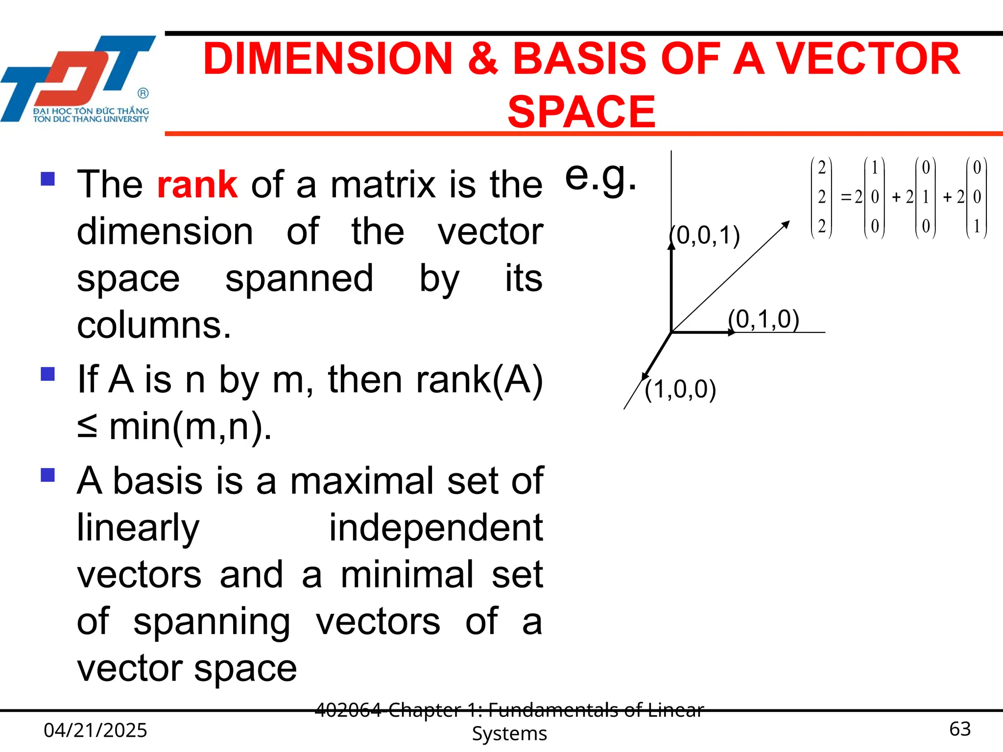
The rank of a matrix is the
dimension of the vector
space spanned by its
columns.
If A is n by m, then rank(A)
≤ min(m,n).
A basis is a maximal set of
linearly independent
vectors and a minimal set
of spanning vectors of a
vector space
64.
DETERMINANTS
04/21/2025
402064-Chapter 1: Fundamentalsof Linear
Systems 64
• Determinants can only be found for square matrices.
• For a 2x2 matrix A, det(A) = ad-bc. Lets have a
closer look at that:
The determinant gives an idea of the ’volume’ occupied by the
matrix in vector space.
A matrix A has an inverse matrix A-1
if and only if det(A)≠0.
a b
c d
det(A) = = ad - bc
[ ]
65.
DETERMINANTS
04/21/2025
402064-Chapter 1: Fundamentalsof Linear
Systems 65
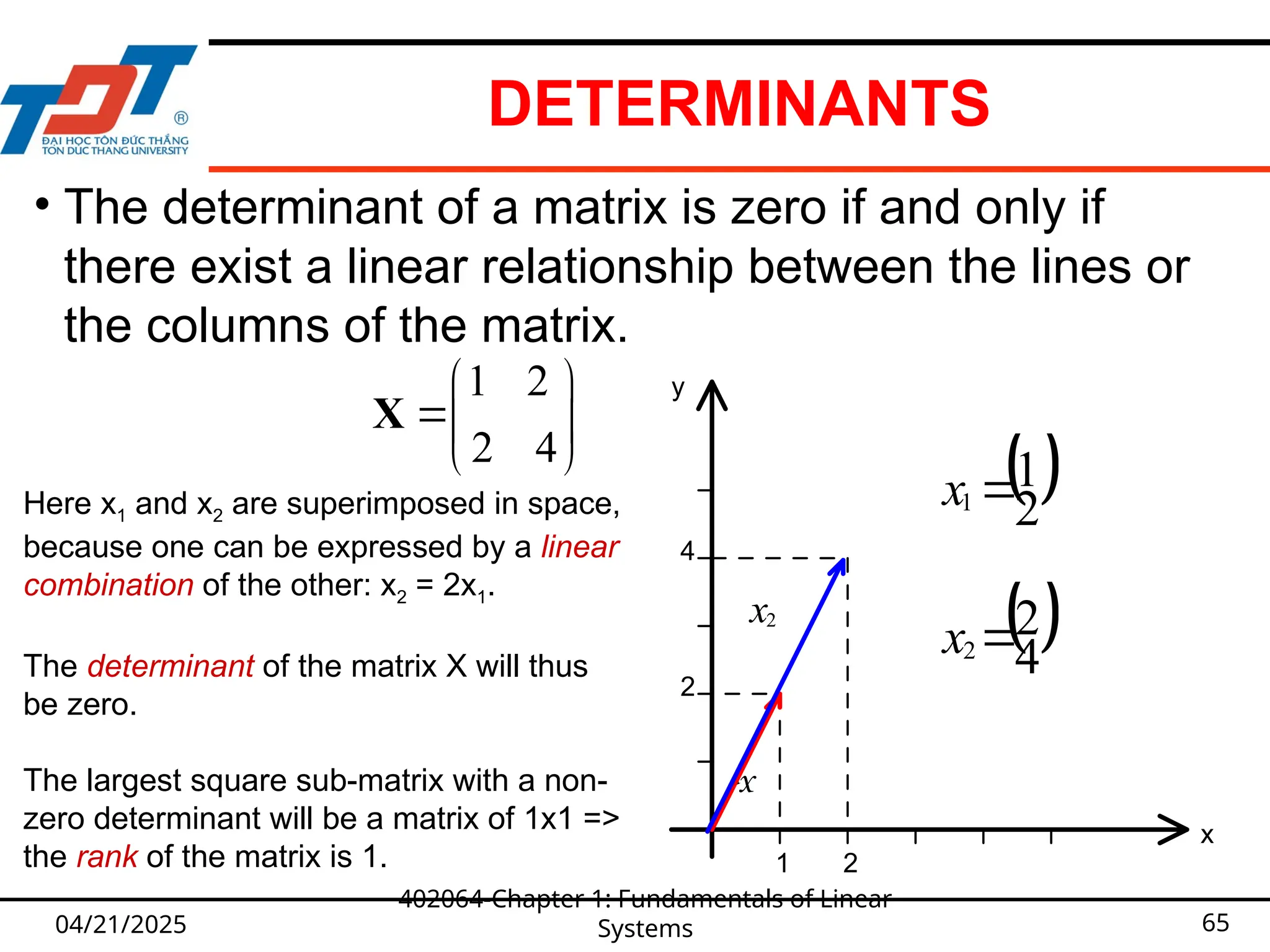
• The determinant of a matrix is zero if and only if
there exist a linear relationship between the lines or
the columns of the matrix.
2
1
1
x
4
2
2
x
2
x
1
x
y
x
4
2
1
2
Here x1 and x2 are superimposed in space,
because one can be expressed by a linear
combination of the other: x2 = 2x1.
The determinant of the matrix X will thus
be zero.
The largest square sub-matrix with a non-
zero determinant will be a matrix of 1x1 =>
the rank of the matrix is 1.
1 2
2 4
X
66.
MATRIX INVERSE
04/21/2025
402064-Chapter 1:Fundamentals of Linear
Systems 66
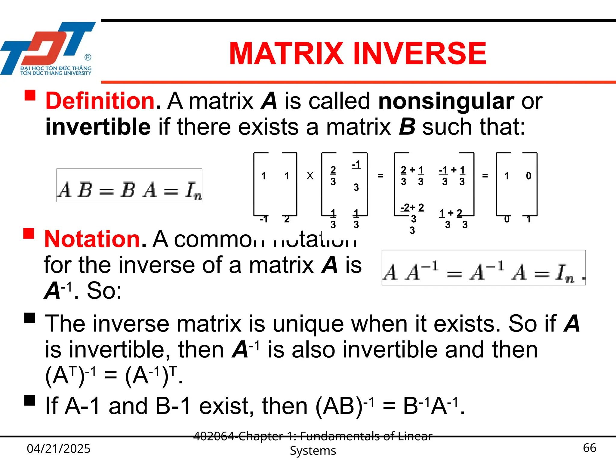
Definition. A matrix A is called nonsingular or
invertible if there exists a matrix B such that:
Notation. A common notation
for the inverse of a matrix A is
A-1
. So:
The inverse matrix is unique when it exists. So if A
is invertible, then A-1
is also invertible and then
(AT
)-1
= (A-1
)T
.
If A-1 and B-1 exist, then (AB)-1
= B-1
A-1
.
1 1 X
2
3
-1
3
=
2 + 1
3 3
-1 + 1
3 3
= 1 0
-1 2
1
3
1
3
-2+ 2
3
3
1 + 2
3 3
0 1
67.
MATRIX INVERSE
04/21/2025
402064-Chapter 1:Fundamentals of Linear
Systems 67
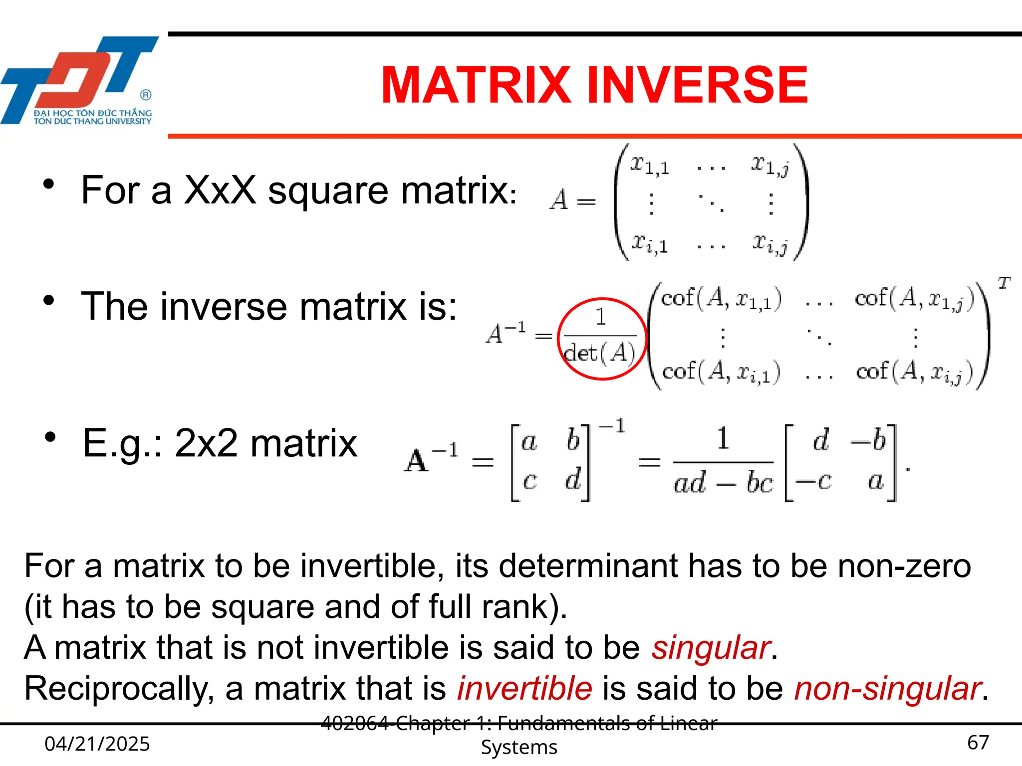
• For a XxX square matrix:
• The inverse matrix is:
• E.g.: 2x2 matrix
For a matrix to be invertible, its determinant has to be non-zero
(it has to be square and of full rank).
A matrix that is not invertible is said to be singular.
Reciprocally, a matrix that is invertible is said to be non-singular.
MATRIX DERIVATIVES -EXAMPLES
04/21/2025
402064-Chapter 1: Fundamentals of Linear
Systems 69
70.
EIGENVALUES & EIGENVECTORS
Definition 1: A nonzero vector x is an eigenvector (or
characteristic vector) of a square matrix A if there
exists a scalar λ such that Ax = λx.
λ is called an eigenvalue (or characteristic value) of A.
Note: The zero vector can not be an eigenvector even
though A.0 = λ.0. But λ = 0 can be an eigenvalue.
04/21/2025
402064-Chapter 1: Fundamentals of Linear
Systems 70
71.
GEOMETRIC INTERPRETATION
Ann×n matrix A multiplied by n×1 vector x results in
another n×1 vector y=Ax. Thus A can be considered
as a transformation matrix.
In general, a matrix acts on a vector by changing both
its magnitude and its direction.
However, a matrix may act on certain vectors by
changing only their magnitude, and leaving their
direction unchanged (or possibly reversing it).
These vectors are the eigenvectors of the matrix.
04/21/2025
402064-Chapter 1: Fundamentals of Linear
Systems 71
72.
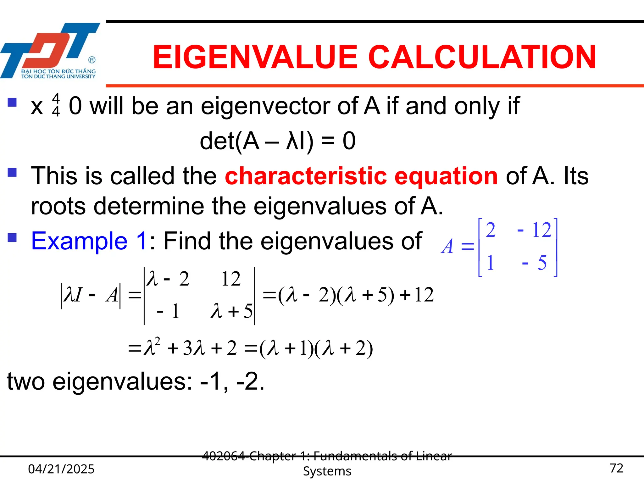
EIGENVALUE CALCULATION
x 0 will be an eigenvector of A if and only if
det(A – λI) = 0
This is called the characteristic equation of A. Its
roots determine the eigenvalues of A.
Example 1: Find the eigenvalues of
two eigenvalues: -1, -2.
04/21/2025
402064-Chapter 1: Fundamentals of Linear
Systems 72
5
1
12
2
A
)
2
)(
1
(
2
3
12
)
5
)(
2
(
5
1
12
2
2
A
I
73.
FINDING EIGENVECTORS
Toeach distinct eigenvalue of a matrix A there are at
least one eigenvector which can be found by solving
the appropriate set of homogenous equations.
If λi is an eigenvalue then the corresponding
eigenvector xi is the solution of (A – λiI)xi = 0.
Example:
04/21/2025
402064-Chapter 1: Fundamentals of Linear
Systems 73
0
0
4
1
4
1
12
3
)
1
(
:
1 A
I
0
,
1
4
,
4
0
4
2
1
1
2
1
2
1
t
t
x
x
t
x
t
x
x
x
x
74.
PROPERTIES
Definition: Thetrace of a matrix A, designated by
tr(A), is the sum of the elements on the main
diagonal.
Property 1: The sum of the eigenvalues of a matrix
equals the trace of the matrix.
Property 2: A matrix is singular if and only if it has a
zero eigenvalue.
Property 3: The eigenvalues of an upper (or lower)
triangular matrix are the elements on the main
diagonal.
04/21/2025
402064-Chapter 1: Fundamentals of Linear
Systems 74
75.
PROPERTIES
Property 4:If λ is an eigenvalue of A then λ is an
eigenvalue of AT
.
Property 5: The product of the eigenvalues (counting
multiplicity) of a matrix equals the determinant of the
matrix.
Property 6: Eigenvectors corresponding to distinct
(that is, different) eigenvalues are linearly
independent.
04/21/2025
402064-Chapter 1: Fundamentals of Linear
Systems 75
76.
SINGULAR VALUE DECOMPOSITION
(SVD)
Any matrix A can be decomposed as A=UDVT
,
where:
D is a diagonal matrix, with d=rank(A) non-zero
elements .
The fist d rows of U are orthogonal basis for col(A).
The fist d rows of V are orthogonal basis for row(A).
Applications of the SVD:
Matrix pseudoinverse
Low-rank matrix approximation
04/21/2025
402064-Chapter 1: Fundamentals of Linear
Systems 76
77.
EIGENVALUE DECOMPOSITION (SVD)
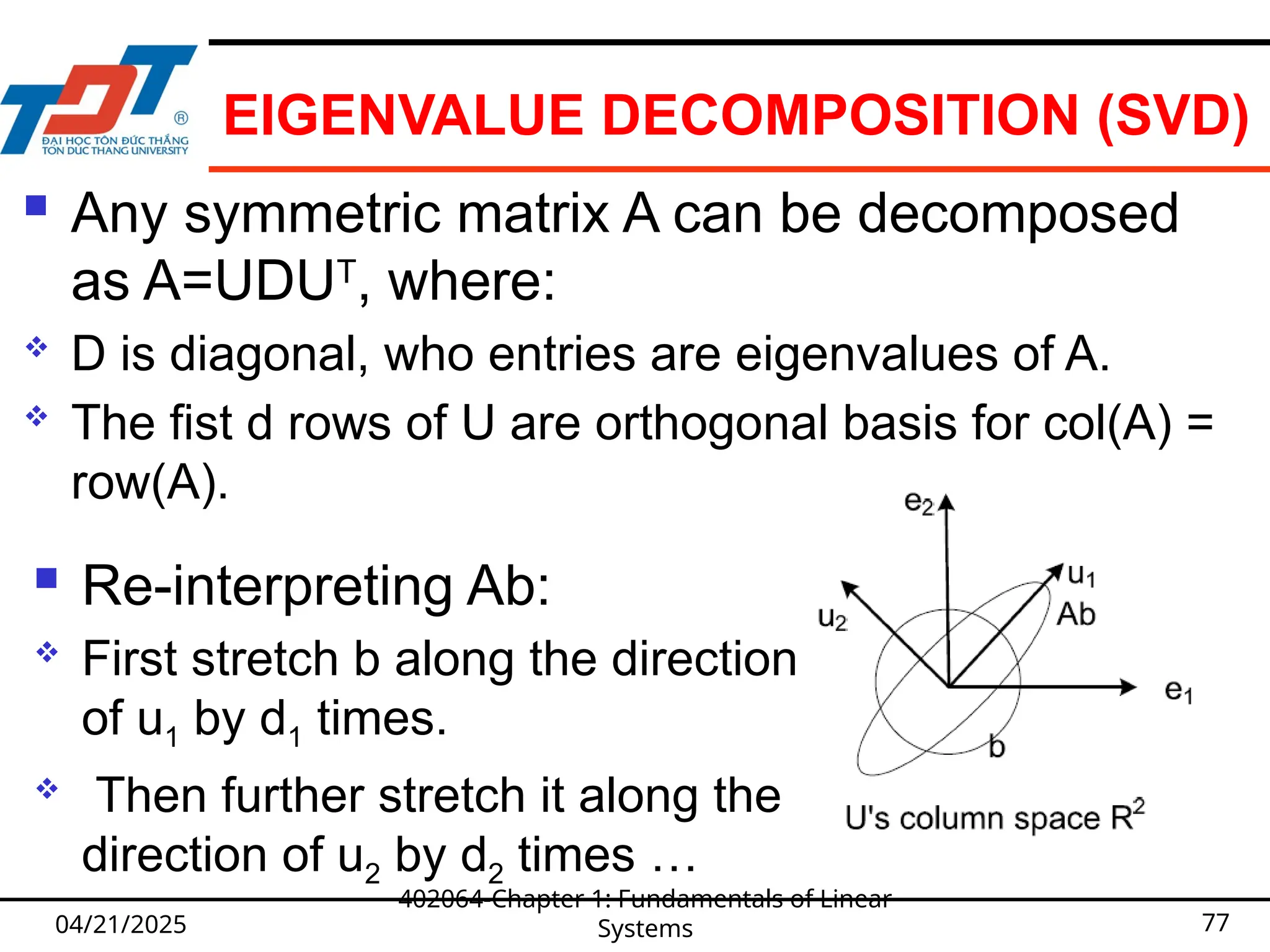
Any symmetric matrix A can be decomposed
as A=UDUT
, where:
D is diagonal, who entries are eigenvalues of A.
The fist d rows of U are orthogonal basis for col(A) =
row(A).
04/21/2025
402064-Chapter 1: Fundamentals of Linear
Systems 77
Re-interpreting Ab:
First stretch b along the direction
of u1 by d1 times.
Then further stretch it along the
direction of u2 by d2 times …
78.
PSEUDOINVERSE
With thehelp of SVD, we actually do NOT
need to explicitly invert XT
X.
Decompose X=UDVT
.
Then XT
X = VDUT
UDVT
= VD2
VT
Since V(D2
)VT
V(D2
)-1
VT
= I
We know that (XT
X)-1
= V(D2
)-1
VT
Inverting a diagonal matrix D2
is trivial.
04/21/2025
402064-Chapter 1: Fundamentals of Linear
Systems 78
79.
WHAT WE HAVELEARNT SO FAR?
So far we have learnt:
Concept of control systems
Classification of control systems
Assignment:
Read more examples in textbook.
Exercises: find more example of control
systems in real life.
04/21/2025
402064-Chapter 1: Fundamentals of Linear
Systems 79
80.
CHAPTER 1: FUNDAMENTALSOF
LINEAR SYSTEMS
1.1 Introduction
1.2 Linear algebra
1.3 Transfer function and impulse response
1.4 Representation of control systems
04/21/2025
402064-Chapter 1: Fundamentals of Linear
Systems 80
81.
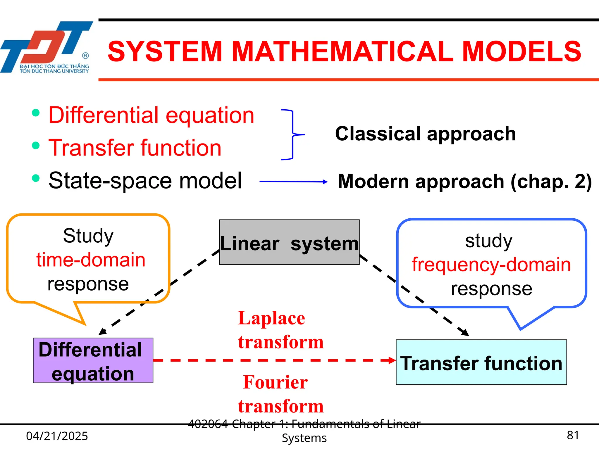
SYSTEM MATHEMATICAL MODELS
04/21/2025
402064-Chapter1: Fundamentals of Linear
Systems 81
Laplace
transform
Differential equation
Transfer function
State-space model
Differential
equation
Transfer function
Linear system
Study
time-domain
response
study
frequency-domain
response
Classical approach
Modern approach (chap. 2)
Fourier
transform
82.
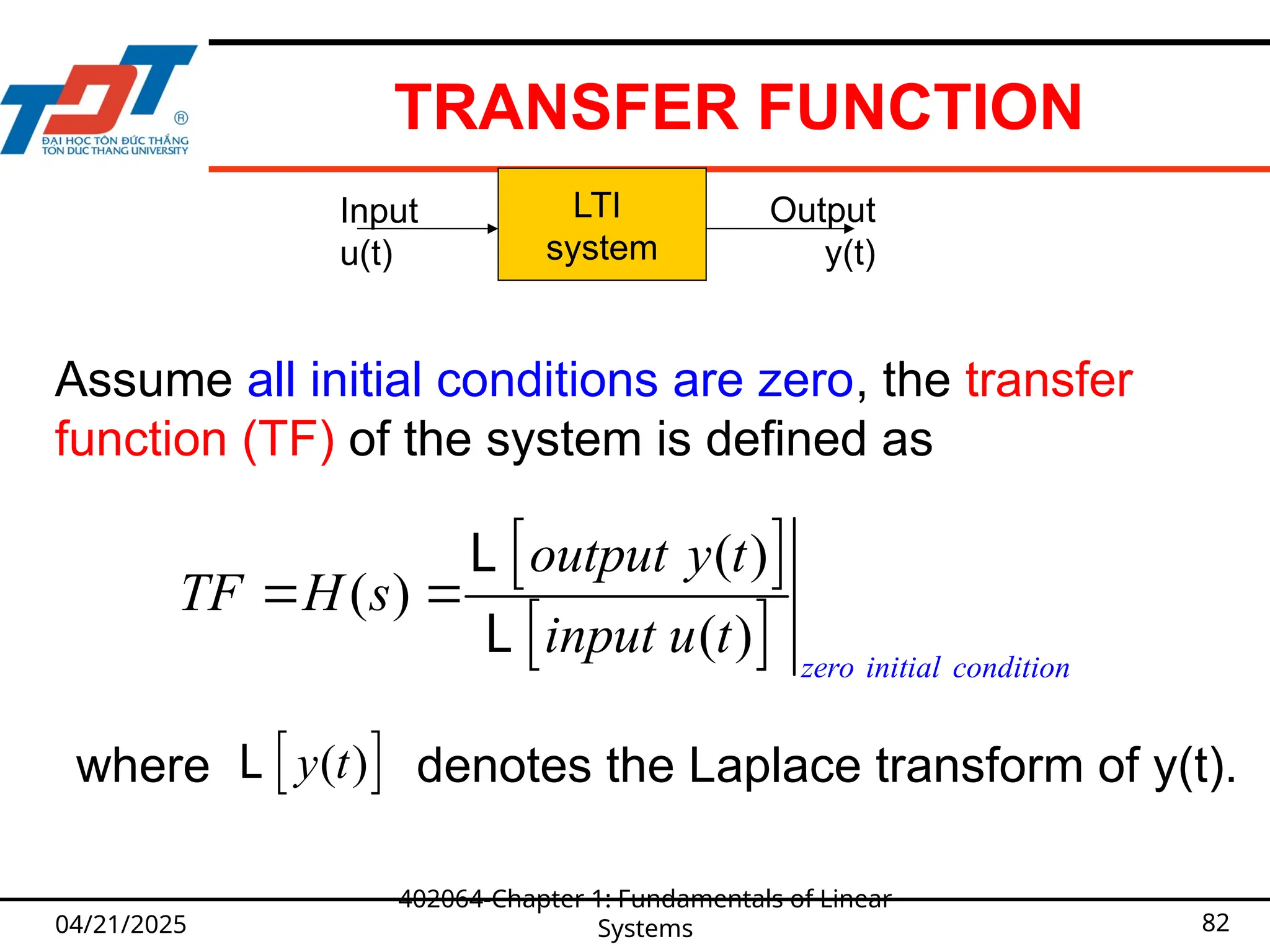
TRANSFER FUNCTION
04/21/2025
402064-Chapter 1:Fundamentals of Linear
Systems 82
LTI
system
Input
u(t)
Output
y(t)
( )
( )
( ) zero initial condition
output y t
TF H s
input u t
L
L
Assume all initial conditions are zero, the transfer
function (TF) of the system is defined as
where denotes the Laplace transform of y(t).
( )
y t
L
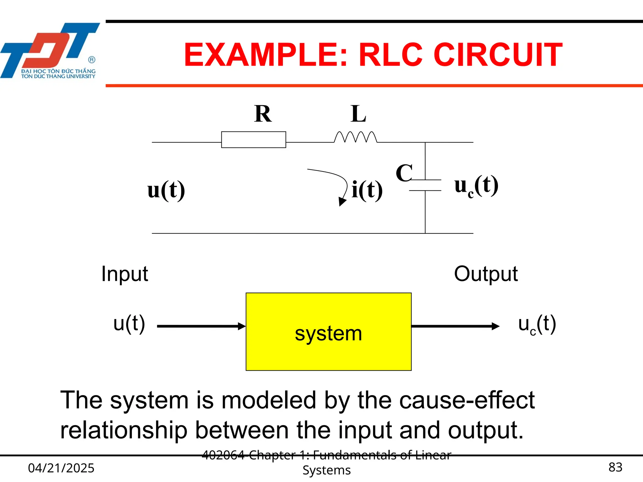
83.
EXAMPLE: RLC CIRCUIT
04/21/202583
R L
C
u(t) uc(t)
i(t)
Input
u(t) system
Output
uc(t)
The system is modeled by the cause-effect
relationship between the input and output.
402064-Chapter 1: Fundamentals of Linear
Systems
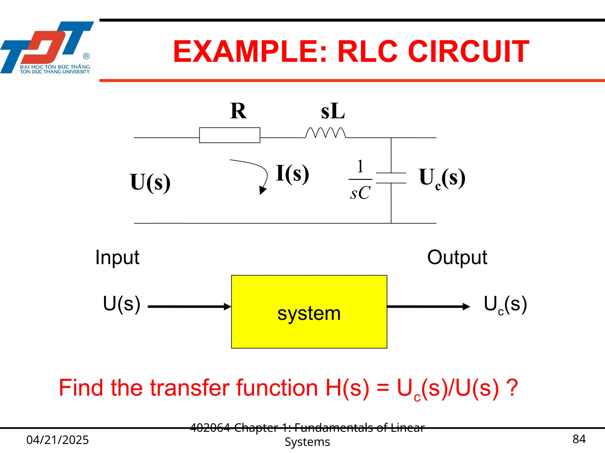
84.
EXAMPLE: RLC CIRCUIT
04/21/202584
R sL
U(s) Uc(s)
I(s)
Input
U(s) system
Output
Uc(s)
Find the transfer function H(s) = Uc(s)/U(s) ?
402064-Chapter 1: Fundamentals of Linear
Systems
1
sC
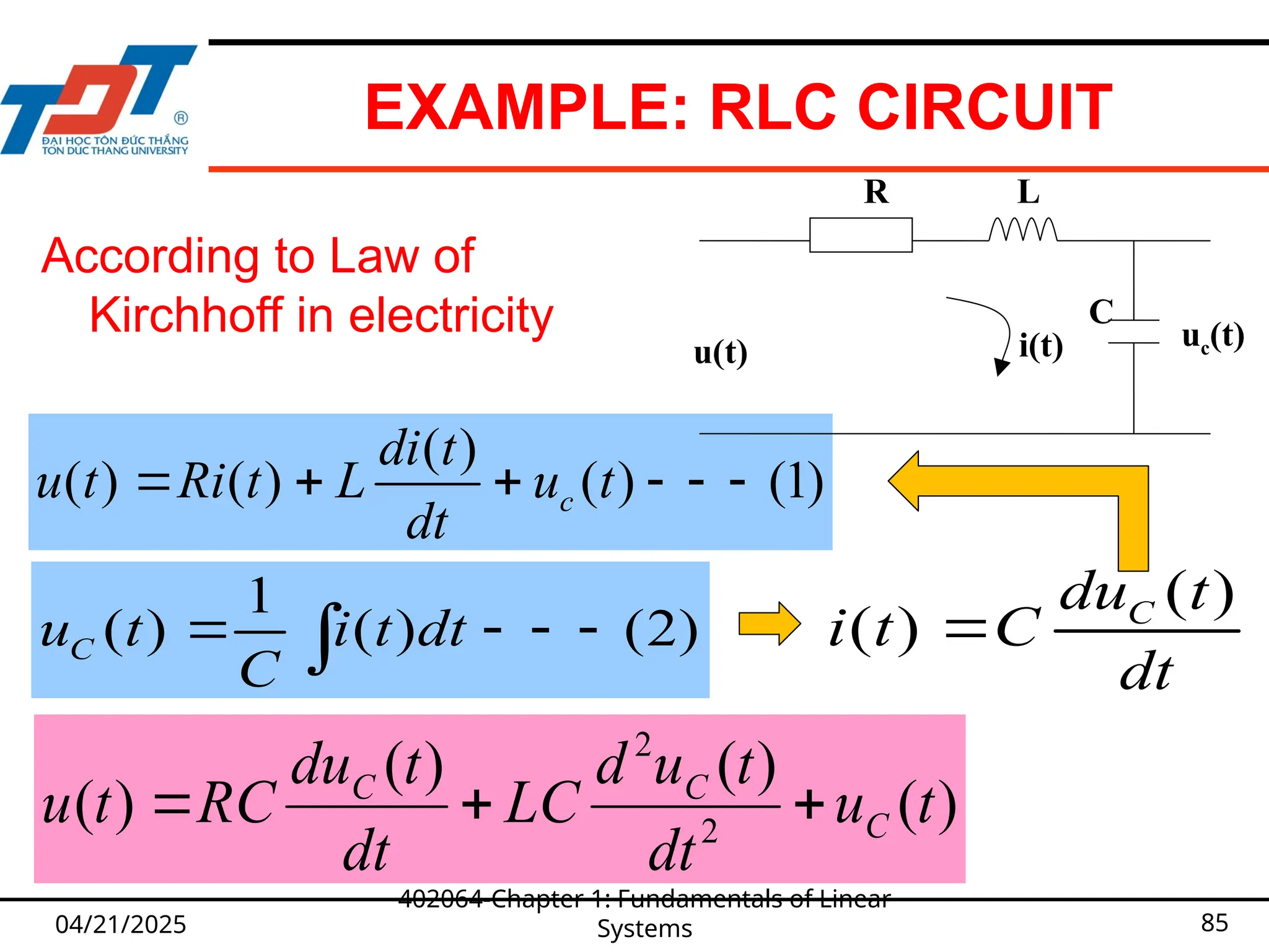
85.
EXAMPLE: RLC CIRCUIT
04/21/202585
)
(
)
(
)
(
)
( 2
2
t
u
dt
t
u
d
LC
dt
t
du
RC
t
u C
C
C
According to Law of
Kirchhoff in electricity
( )
( ) ( ) ( ) (1)
c
di t
u t Ri t L u t
dt
1
( ) ( ) (2)
C
u t i t dt
C
( )
( ) C
du t
i t C
dt
R L
C
u(t) uc(t)
i(t)
402064-Chapter 1: Fundamentals of Linear
Systems
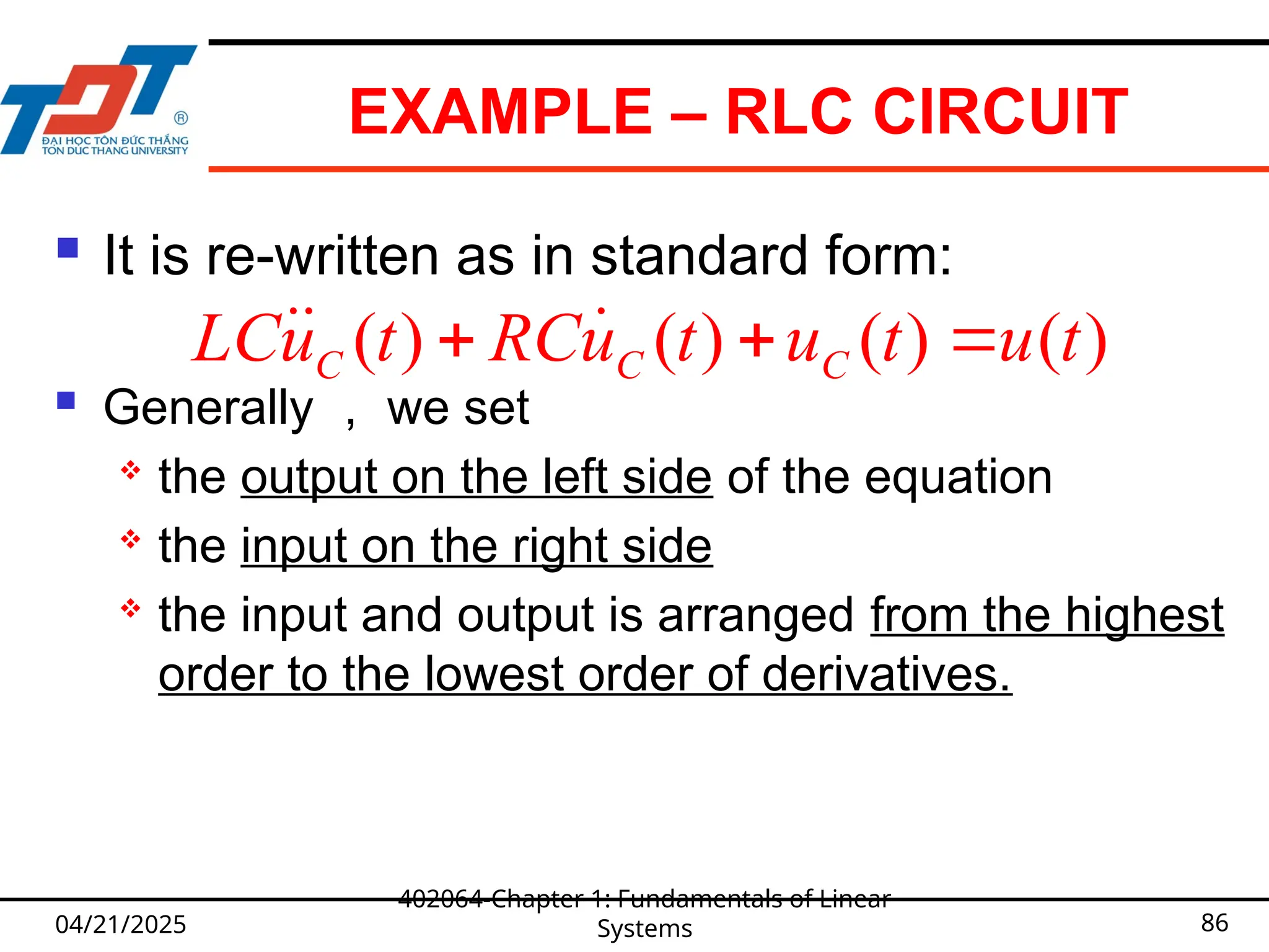
86.
EXAMPLE – RLCCIRCUIT
It is re-written as in standard form:
Generally , we set
the output on the left side of the equation
the input on the right side
the input and output is arranged from the highest
order to the lowest order of derivatives.
04/21/2025
402064-Chapter 1: Fundamentals of Linear
Systems 86
( ) ( ) ( ) ( )
C C C
LCu t RCu t u t u t
87.
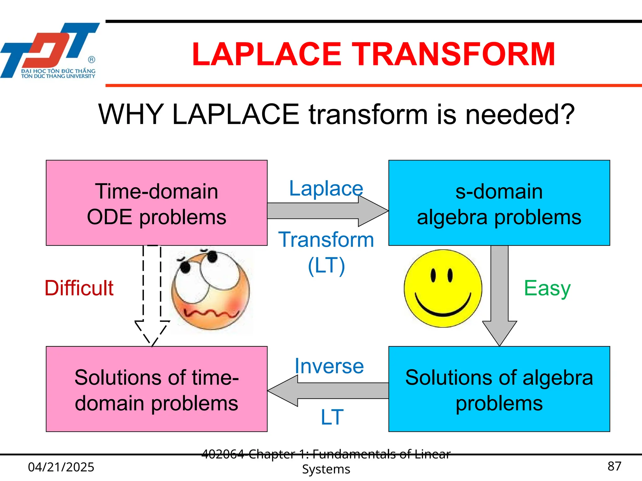
LAPLACE TRANSFORM
04/21/2025
402064-Chapter 1:Fundamentals of Linear
Systems 87
WHY LAPLACE transform is needed?
s-domain
algebra problems
Solutions of algebra
problems
Time-domain
ODE problems
Solutions of time-
domain problems
Laplace
Transform
(LT)
Inverse
LT
Difficult Easy
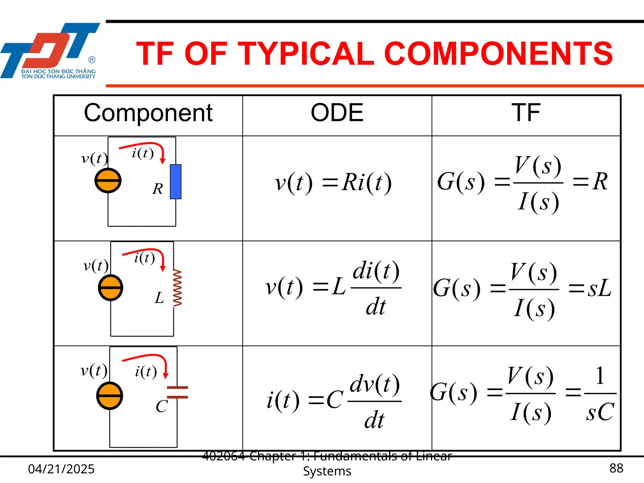
88.
TF OF TYPICALCOMPONENTS
04/21/2025
402064-Chapter 1: Fundamentals of Linear
Systems 88
Component ODE TF
( )
v t ( )
i t
R ( ) ( )
v t Ri t
( )
( )
( )
V s
G s R
I s
( )
v t
( )
i t
L
( )
( )
di t
v t L
dt
( )
( )
( )
V s
G s sL
I s
( )
v t ( )
i t
C
( )
( )
dv t
i t C
dt
( ) 1
( )
( )
V s
G s
I s sC
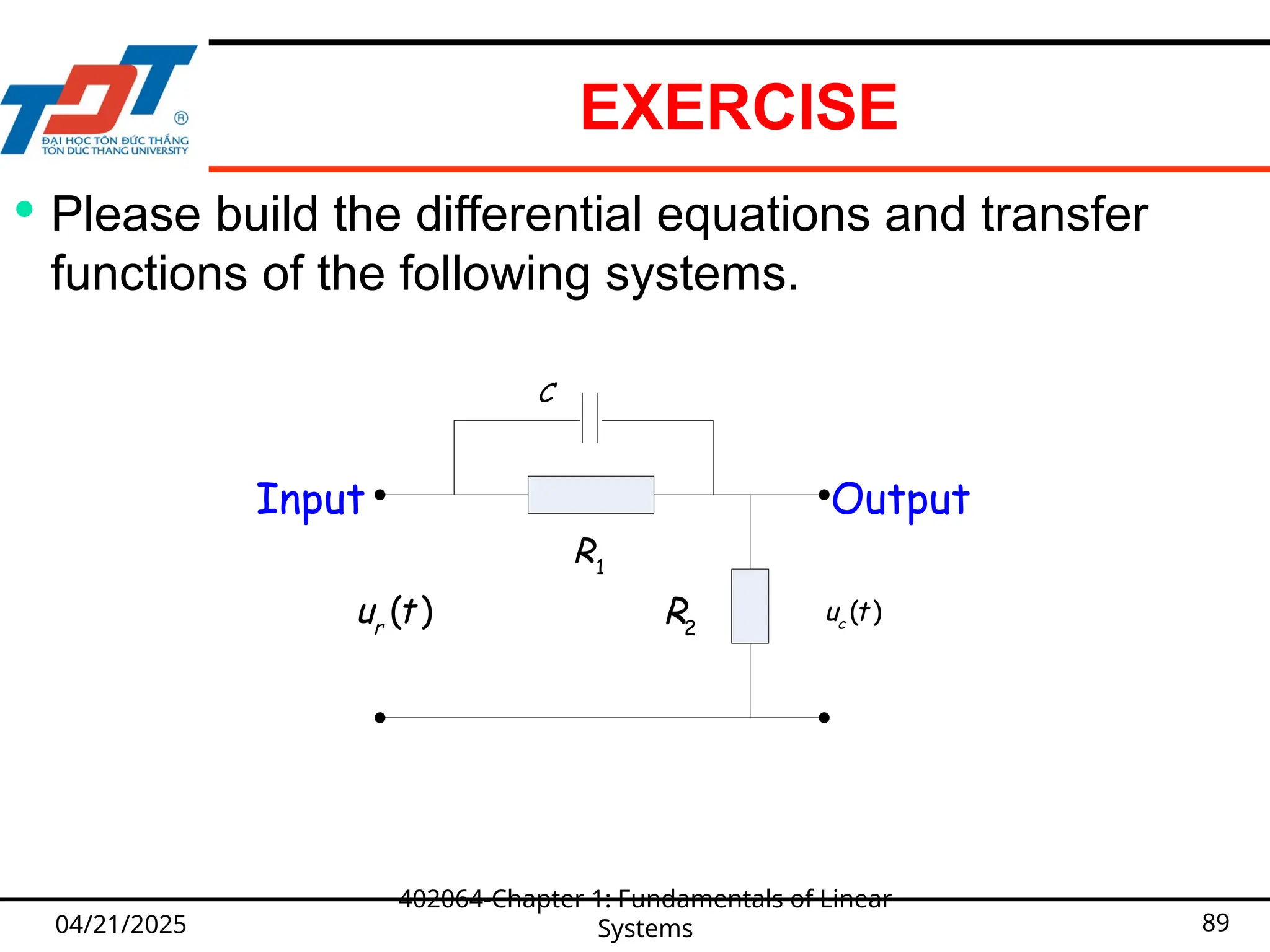
89.
EXERCISE
04/21/2025
402064-Chapter 1: Fundamentalsof Linear
Systems 89
Please build the differential equations and transfer
functions of the following systems.
Output
Input
1
R
2
R
C
( )
r
u t ( )
c
u t
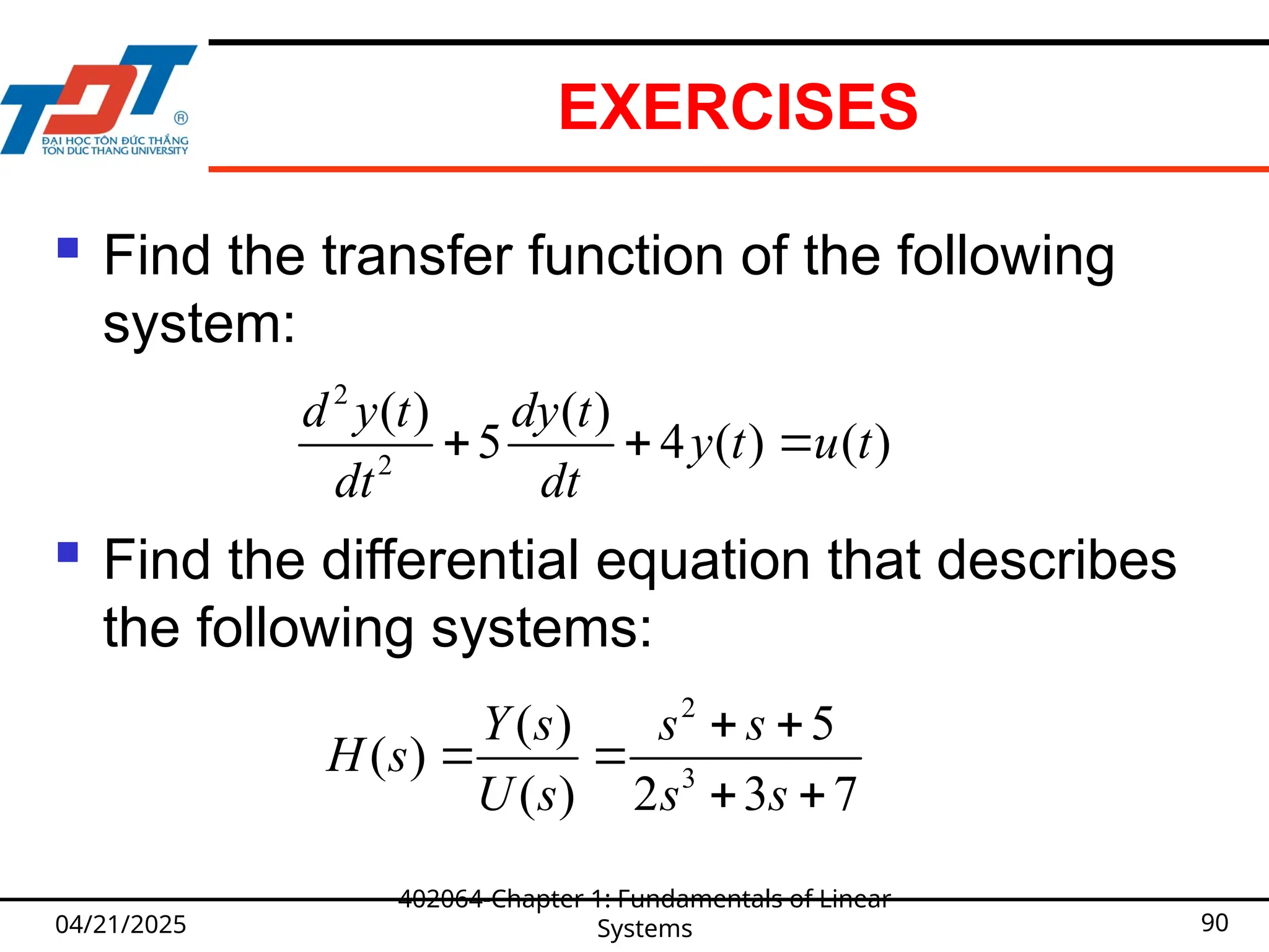
90.
EXERCISES
Find thetransfer function of the following
system:
Find the differential equation that describes
the following systems:
04/21/2025
402064-Chapter 1: Fundamentals of Linear
Systems 90
2
2
( ) ( )
5 4 ( ) ( )
d y t dy t
y t u t
dt dt
2
3
( ) 5
( )
( ) 2 3 7
Y s s s
H s
U s s s
91.
PROPERTIES OF TRANSFER
FUNCTION
The transfer function is defined only for a linear
time-invariant system, not for nonlinear system.
All initial conditions of the system are set to zero.
The transfer function is independent of the input of
the system.
The transfer function G(s) is the Laplace transform
of the unit impulse response g(t).
04/21/2025
402064-Chapter 1: Fundamentals of Linear
Systems 91
92.
IMPULSE RESPONSE
Considerthe output of a LTI system to a unit-
impulse input when the initial conditions are zero.
The Laplace transform of the output of the system is
Y(s) = G(s).1 = G(s) (since the Laplace transform of
the unit-impulse function is unity)
Definition: the inverse Laplace transform of G(s),
or , is called the impulse-response
function of the system.
04/21/2025
402064-Chapter 1: Fundamentals of Linear
Systems 92
1
[ ( )] g(t)
G s
L
93.
REVIEW QUESTIONS AND
ASSIGNMENTS
Review questions:
What is the definition of “transfer function”?
When defining the transfer function, what happens
to initial conditions of the system?
Does a nonlinear system have a transfer function?
How does a transfer function of a LTI system relate
to its impulse response?
Assignments: B-2-9 and the exercises from
next slide.
04/21/2025
402064-Chapter 1: Fundamentals of Linear
Systems 93
94.
CHAPTER 1: FUNDAMENTALSOF
LINEAR SYSTEMS
1.1 Introduction
1.2 Linear algebra
1.3 Transfer function and impulse response
1.4 Representation of control systems
04/21/2025
402064-Chapter 1: Fundamentals of Linear
Systems 94
95.
BLOCK DIAGRAM OFLTI CONTROL
SYSTEMS
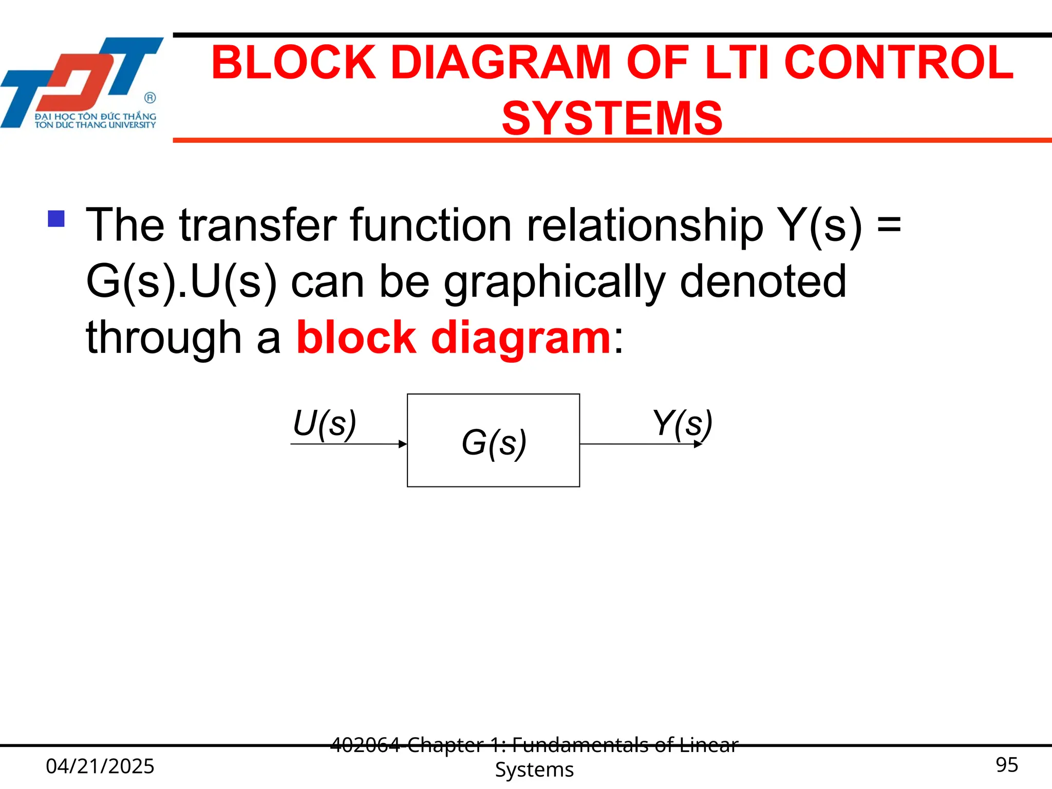
The transfer function relationship Y(s) =
G(s).U(s) can be graphically denoted
through a block diagram:
04/21/2025
402064-Chapter 1: Fundamentals of Linear
Systems 95
G(s)
U(s) Y(s)
96.
EQUIVALENT TRANSFORM OF
BLOCKDIAGRAM
04/21/2025
402064-Chapter 1: Fundamentals of Linear
Systems 96
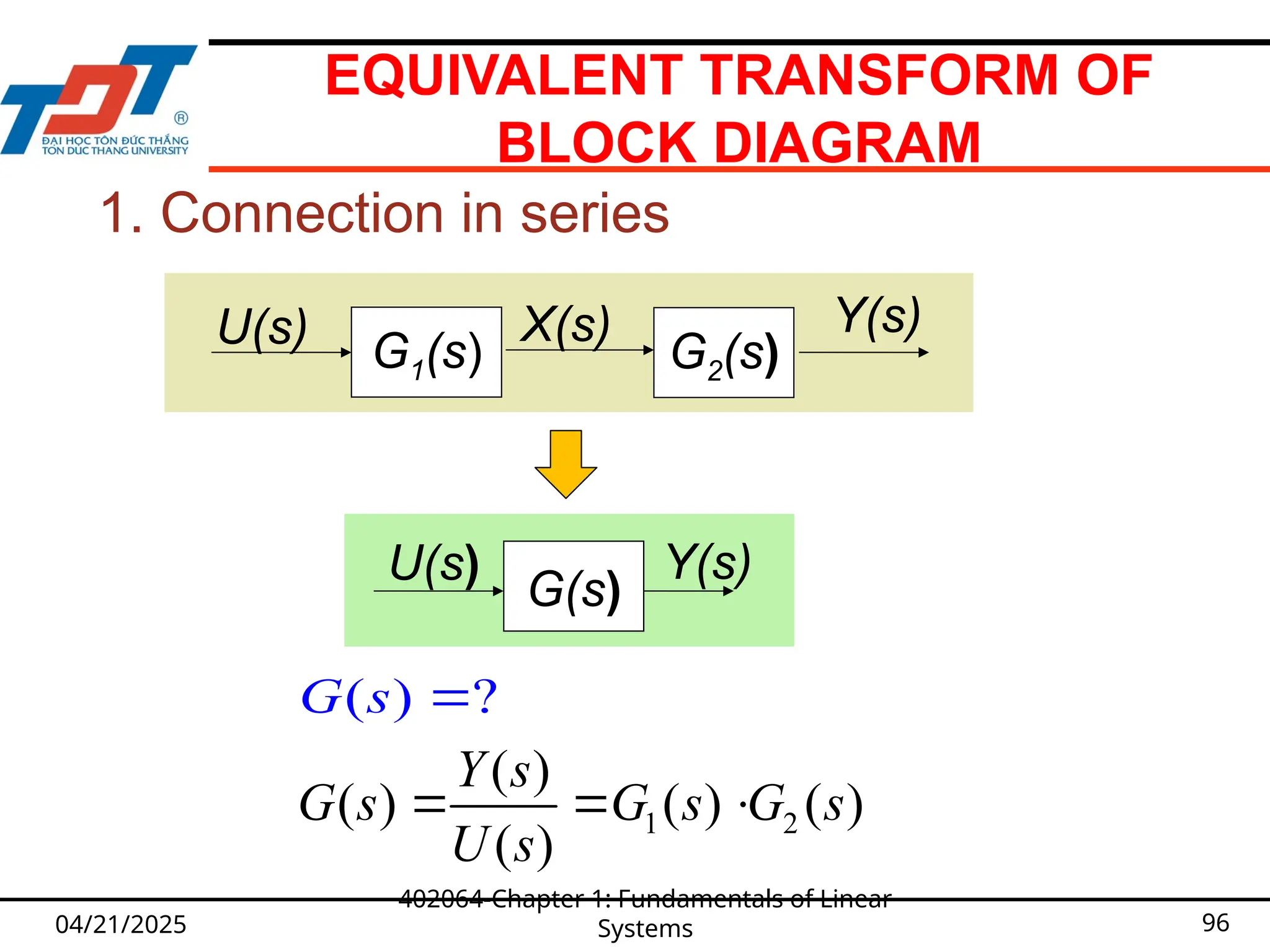
1. Connection in series
G(s)
U(s) Y(s)
( ) ?
G s
X(s)
G1(s) G2(s)
U(s) Y(s)
1 2
( )
( ) ( ) ( )
( )
Y s
G s G s G s
U s
97.
EQUIVALENT TRANSFORM OF
BLOCKDIAGRAM
04/21/2025
402064-Chapter 1: Fundamentals of Linear
Systems 97
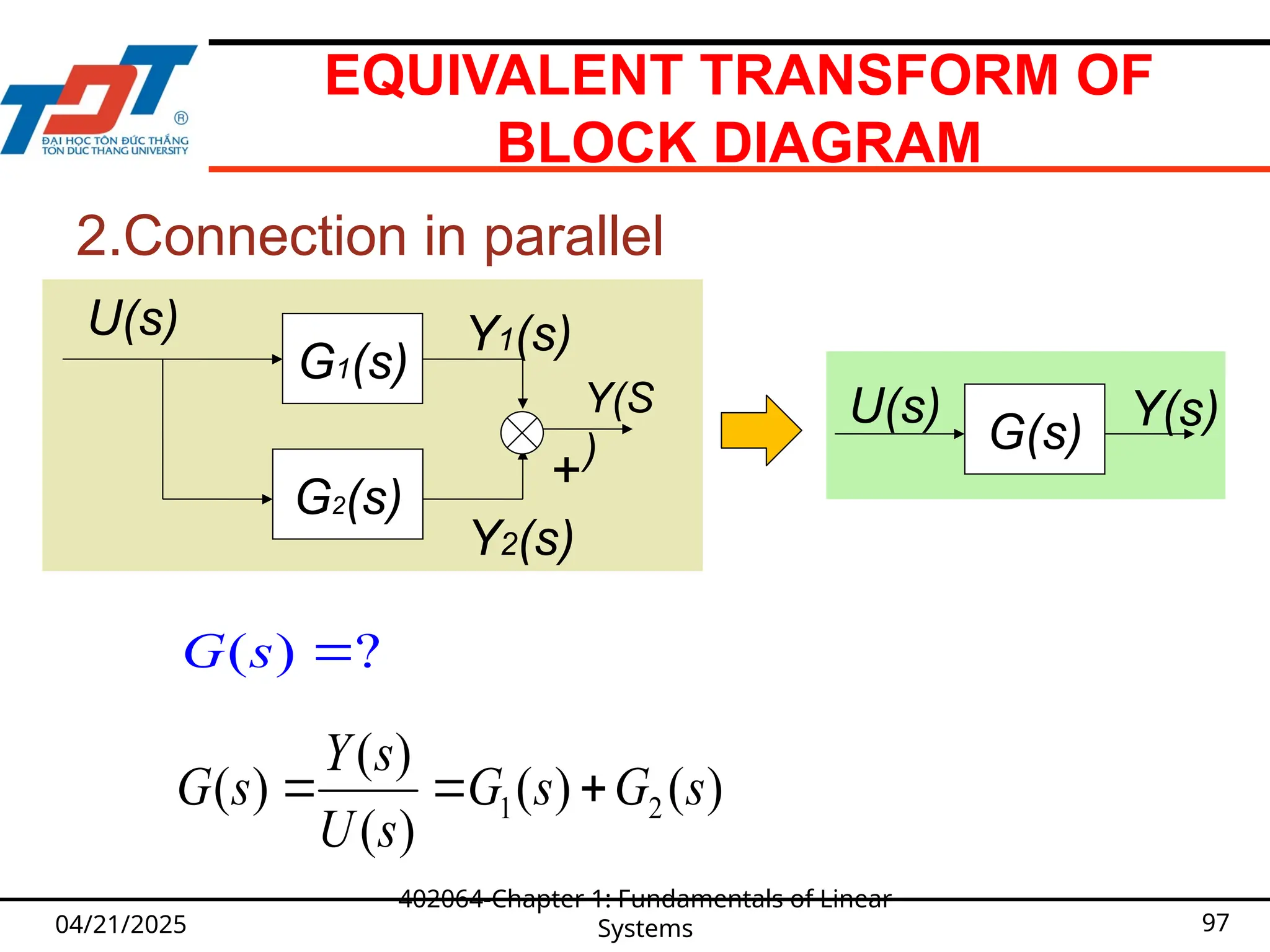
2.Connection in parallel
G(s)
U(s) Y(s)
1 2
( )
( ) ( ) ( )
( )
Y s
G s G s G s
U s
U(s)
G2(s)
G1(s)
Y1(s)
Y2(s)
Y(S
)
( ) ?
G s
98.
EQUIVALENT TRANSFORM OF
BLOCKDIAGRAM
04/21/2025
402064-Chapter 1: Fundamentals of Linear
Systems 98
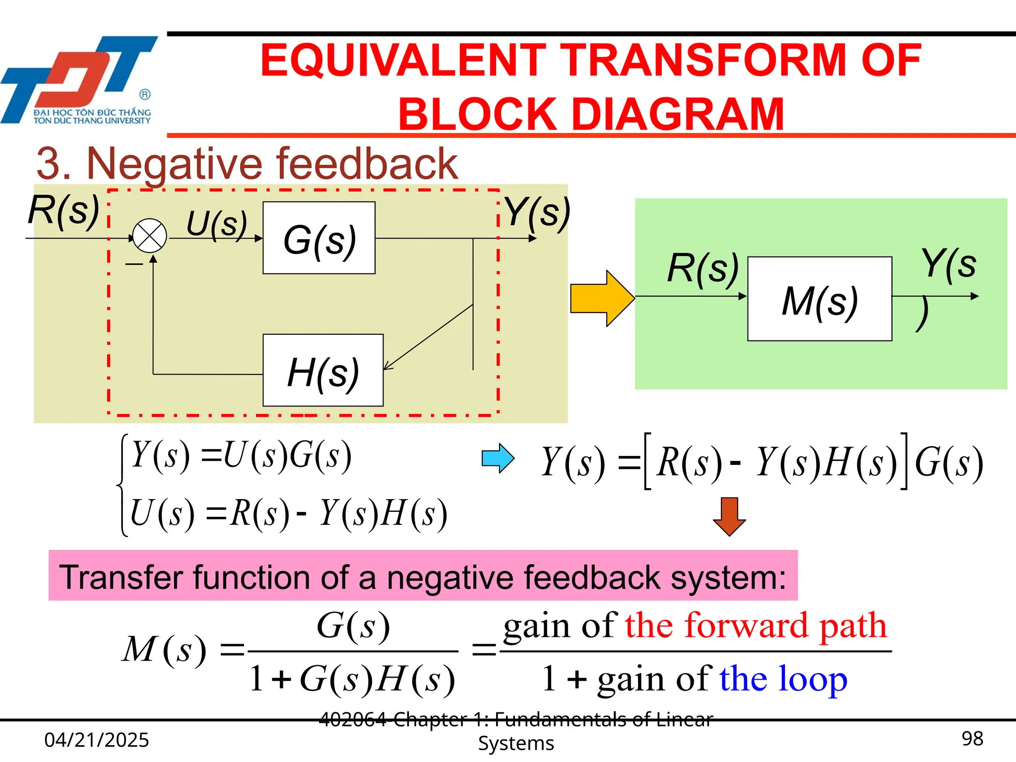
3. Negative feedback
M(s)
R(s) Y(s
)
( ) ( ) ( )
( ) ( ) ( ) ( )
Y s U s G s
U s R s Y s H s
the for
( w
) a
gain of
( )
1
rd path
( ) ( ) 1 gai the loop
n of
G s
M s
G s H s
( ) ( ) ( ) ( ) ( )
Y s R s Y s H s G s
Y(s)
G(s)
H(s)
U(s)
R(s)
_
Transfer function of a negative feedback system:
99.
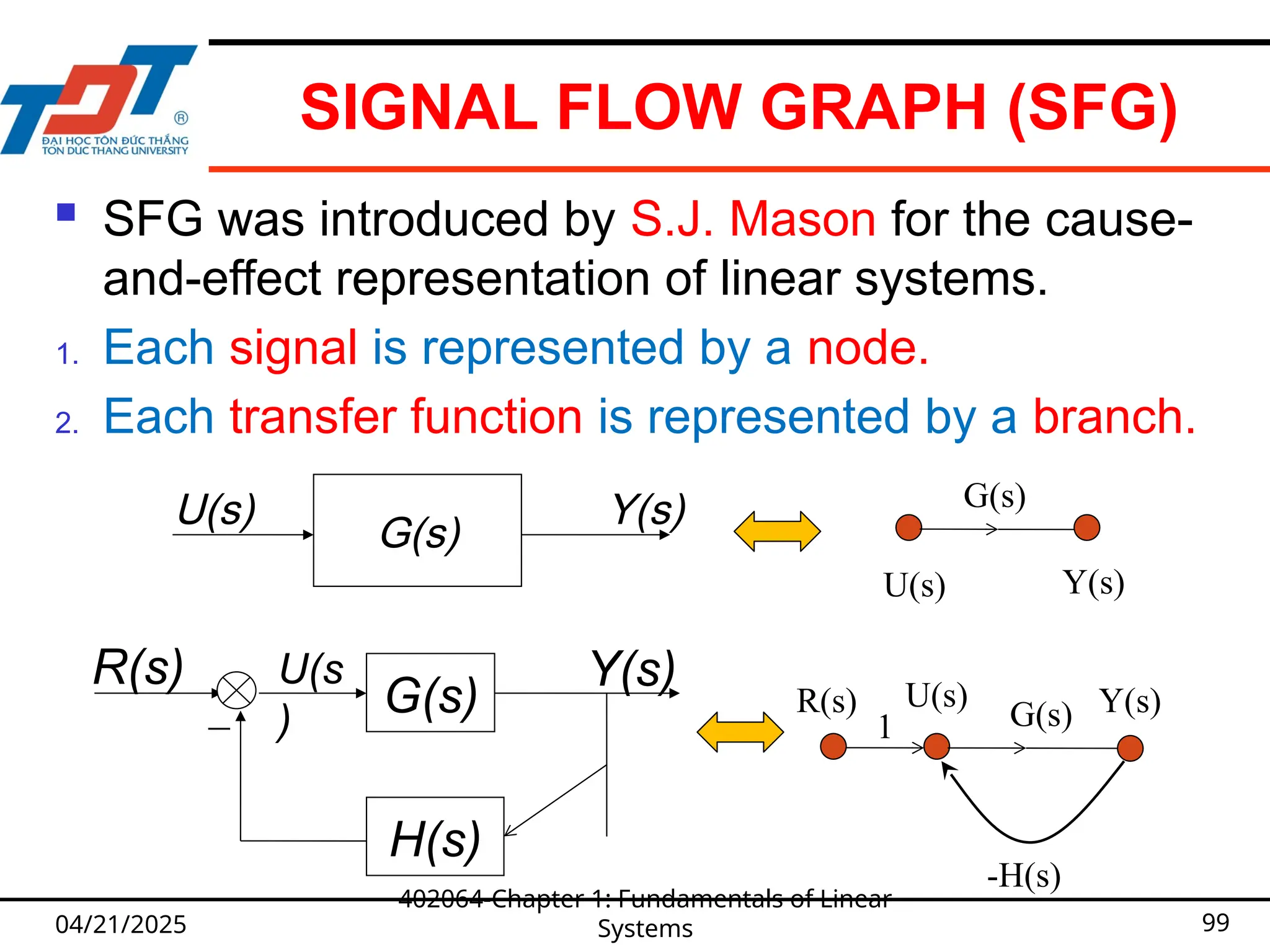
SIGNAL FLOW GRAPH(SFG)
SFG was introduced by S.J. Mason for the cause-
and-effect representation of linear systems.
1. Each signal is represented by a node.
2. Each transfer function is represented by a branch.
04/21/2025
402064-Chapter 1: Fundamentals of Linear
Systems 99
G(s)
U(s) Y(s)
G(s)
H(s)
U(s
)
R(s)
_
Y(s)
G(s)
U(s) Y(s)
G(s)
U(s) Y(s)
R(s)
-H(s)
1
100.
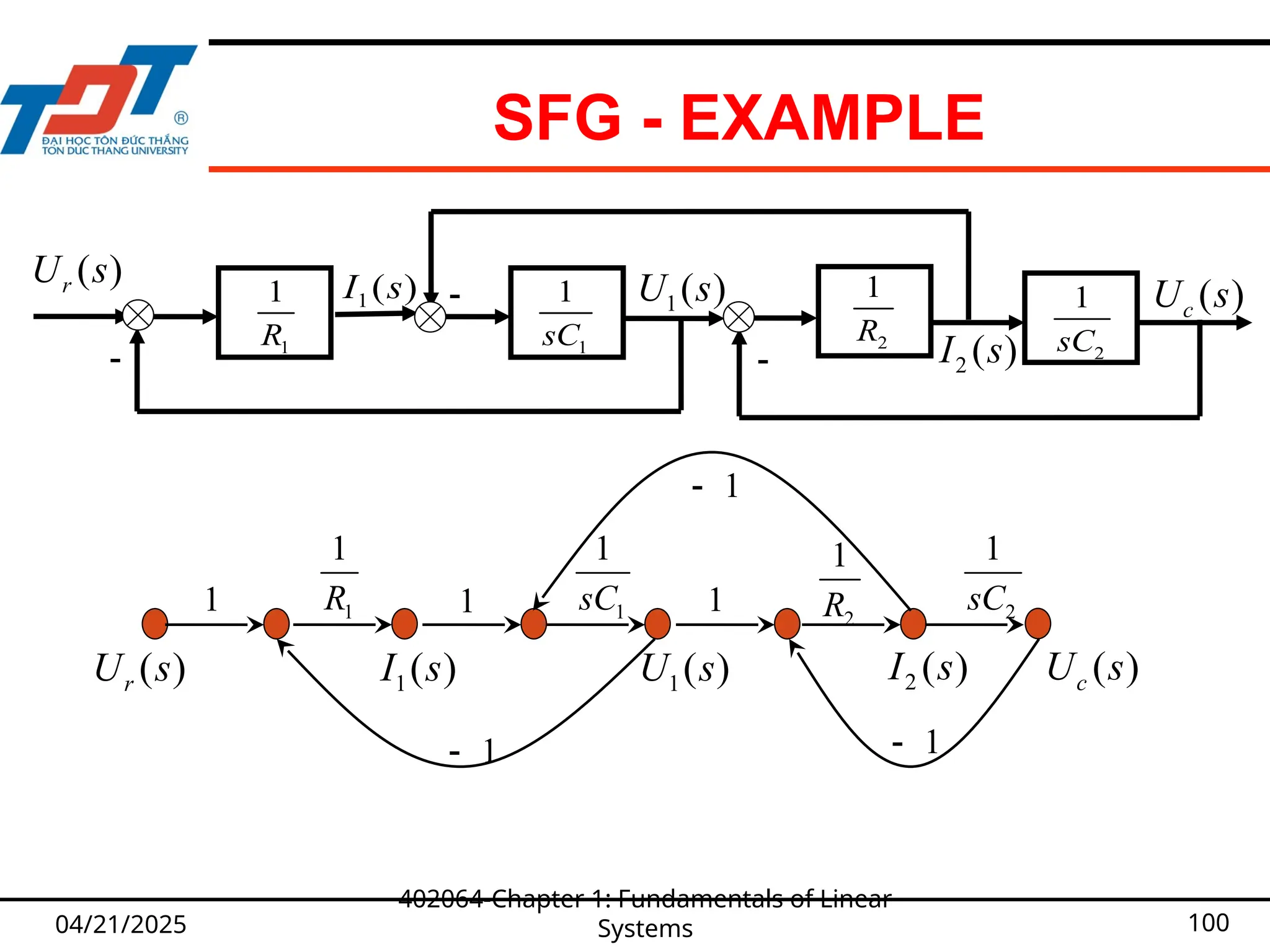
SFG - EXAMPLE
04/21/2025
402064-Chapter1: Fundamentals of Linear
Systems 100
( )
r
U s
1 ( )
I s
2 ( )
I s
( )
c
U s
1( )
U s
- 1
1
R 1
1
sC
-
2
1
R
- 2
1
sC
( )
r
U s 1( )
I s 1( )
U s 2 ( )
I s ( )
c
U s
1
1
R 1
1
sC 2
1
R 2
1
sC
- 1 - 1
- 1
1 1 1
101.
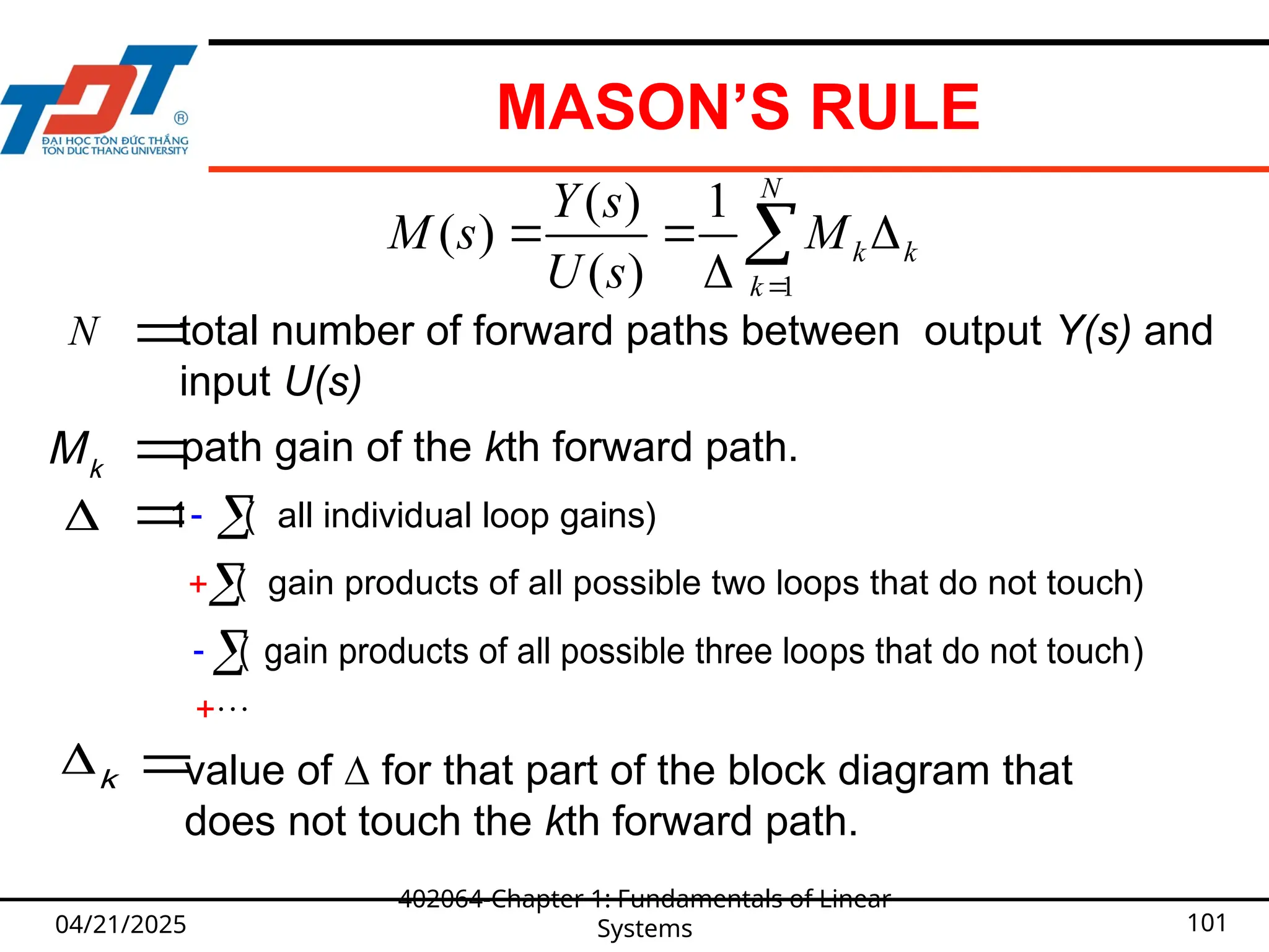
MASON’S RULE
04/21/2025
402064-Chapter 1:Fundamentals of Linear
Systems 101
1
( ) 1
( )
( )
N
k k
k
Y s
M s M
U s
k
M path gain of the kth forward path.
1 ( all individual loop gains)
( gain products of all possible three loops that do not touch)
( gain products of all possible two loops that do not touch)
k
value of ∆ for that part of the block diagram that
does not touch the kth forward path.
N
total number of forward paths between output Y(s) and
input U(s)
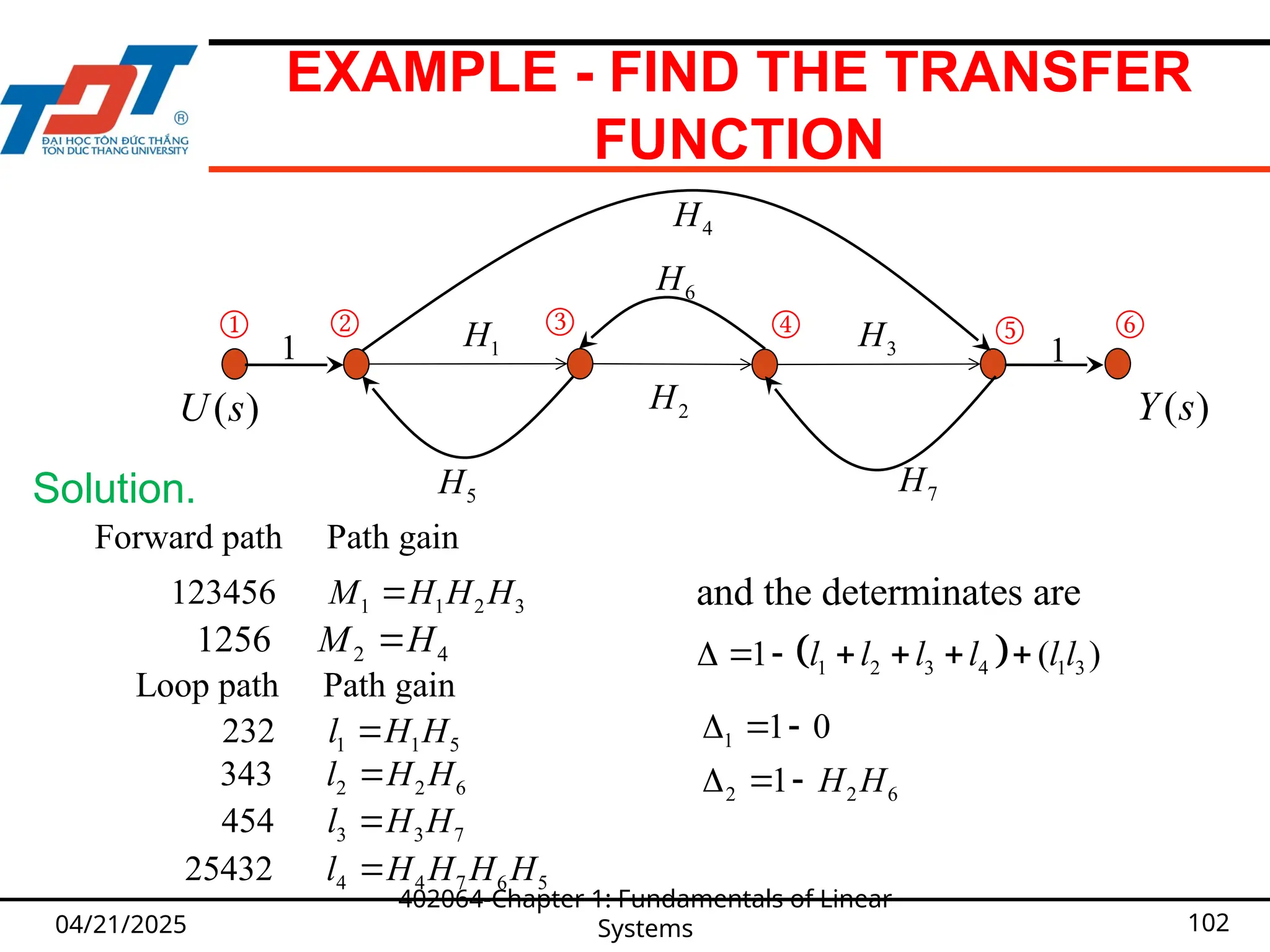
102.
EXAMPLE - FINDTHE TRANSFER
FUNCTION
04/21/2025
402064-Chapter 1: Fundamentals of Linear
Systems 102
Solution.
Forward path Path gain
and the determinates are
1 1 2 3
123456 M H H H
2 4
1256 M H
Loop path Path gain
1 1 5
232 l H H
2 2 6
343 l H H
3 3 7
454 l H H
4 4 7 6 5
25432 l H H H H
1 2 3 4 1 3
1 ( )
l l l l l l
1
2 2 6
1 0
1 H H
( )
U s ( )
Y s
5
H
1 1
H
4
H
6
H
7
H
2
H
3
H 1
① ② ③ ④ ⑤ ⑥
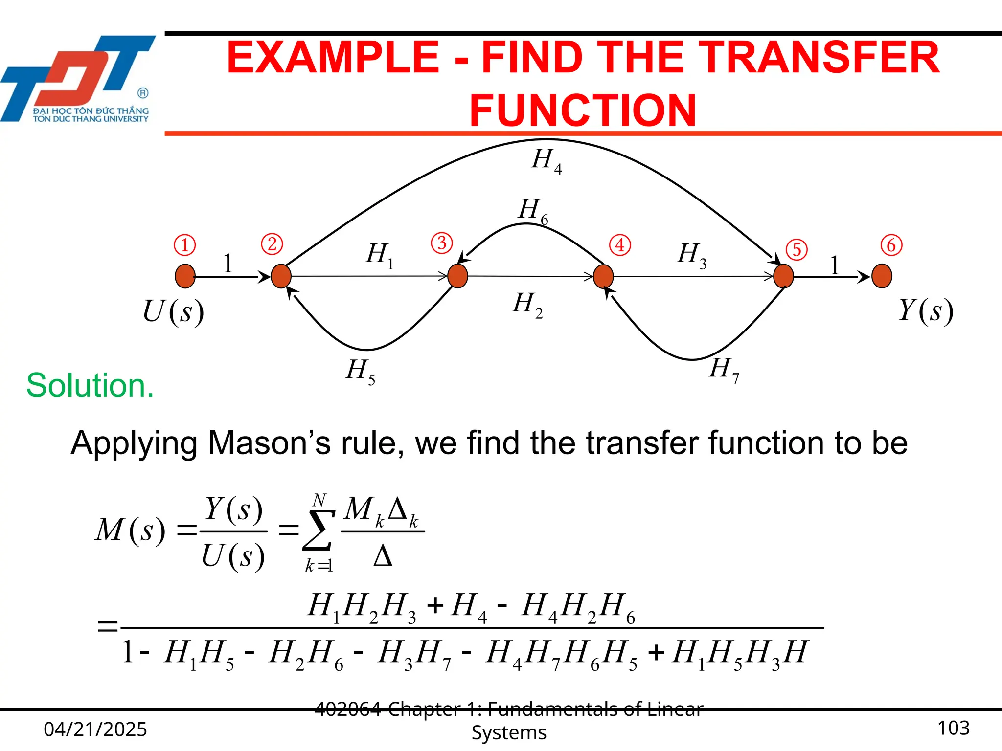
103.
EXAMPLE - FINDTHE TRANSFER
FUNCTION
04/21/2025
402064-Chapter 1: Fundamentals of Linear
Systems 103
Solution.
( )
U s ( )
Y s
5
H
1 1
H
4
H
6
H
7
H
2
H
3
H 1
① ② ③ ④ ⑤ ⑥
1
1 2 3 4 4 2 6
1 5 2 6 3 7 4 7 6 5 1 5 3
( )
( )
( )
1
N
k k
k
M
Y s
M s
U s
H H H H H H H
H H H H H H H H H H H H H H
Applying Mason’s rule, we find the transfer function to be
104.
SUMMARY AND ASSIGNMENT
In this chapter, we have learnt:
Basic concept and classification of control
systems.
Review of linear algebra
Mathematical model of LTI systems
Graphical representation of LTI systems.
Assignments: B-2-5 to B-2-8.
Reading assignment: Ogata - chapter 2 (pp.
29-39).
04/21/2025
402064-Chapter 1: Fundamentals of Linear
Systems 104
![TYPES OF CONTROL SYSTEMS
In continuous data control system all system
variables are function of a continuous time t.
A discrete time control system involves one or more
variables that are known only at discrete time
intervals.
04/21/2025
402064-Chapter 1: Fundamentals of Linear
Systems 30
x(t)
t
X[n]
n](https://image.slidesharecdn.com/402064-engineeringanalysis-chapter1-250421115507-2acf725b/75/402064-ENGINEERING-ANALYSIS-CHAPTER-1-pptx-30-2048.jpg)

![DETERMINANTS
04/21/2025
402064-Chapter 1: Fundamentals of Linear
Systems 64
• Determinants can only be found for square matrices.
• For a 2x2 matrix A, det(A) = ad-bc. Lets have a
closer look at that:
The determinant gives an idea of the ’volume’ occupied by the
matrix in vector space.
A matrix A has an inverse matrix A-1
if and only if det(A)≠0.
a b
c d
det(A) = = ad - bc
[ ]](https://image.slidesharecdn.com/402064-engineeringanalysis-chapter1-250421115507-2acf725b/75/402064-ENGINEERING-ANALYSIS-CHAPTER-1-pptx-64-2048.jpg)

![IMPULSE RESPONSE
Consider the output of a LTI system to a unit-
impulse input when the initial conditions are zero.
The Laplace transform of the output of the system is
Y(s) = G(s).1 = G(s) (since the Laplace transform of
the unit-impulse function is unity)
Definition: the inverse Laplace transform of G(s),
or , is called the impulse-response
function of the system.
04/21/2025
402064-Chapter 1: Fundamentals of Linear
Systems 92
1
[ ( )] g(t)
G s
L](https://image.slidesharecdn.com/402064-engineeringanalysis-chapter1-250421115507-2acf725b/75/402064-ENGINEERING-ANALYSIS-CHAPTER-1-pptx-92-2048.jpg)