good

1. Fluid Mechanics-II by Dr.-Ing. S. Mushahid Hashmi (Lecture 5- Reynold’s Transport Theorem-Continuity equation)
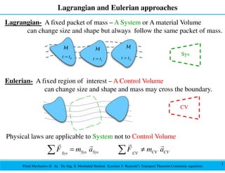
Lagrangian and Eulerian approaches
1
Physical laws are applicable to System not to Control Volume
Sys Sys CV CV
Sys CV
F m a F m a
= ≠
∑ ∑
r r
r r
Eulerian- A fixed region of interest – A Control Volume
can change size and shape and mass may cross the boundary.
CV
Lagrangian- A fixed packet of mass – A System or A material Volume
can change size and shape but always follow the same packet of mass.
Sys

2. Fluid Mechanics-II by Dr.-Ing. S. Mushahid Hashmi (Lecture 5- Reynold’s Transport Theorem-Continuity equation)
System and Control Volume- Quiz
2
In a System approach we follow the
fluid as it moves and deforms.
No mass crosses the boundary, and the
total mass of the system remains fixed.
In a Control Volume approach we
consider a fixed interior volume.
Mass crosses the boundary.
A B
Which approach is
Control volume?
A or B
Analyzing spraying of deodorant from a spray can

3. Fluid Mechanics-II by Dr.-Ing. S. Mushahid Hashmi (Lecture 5- Reynold’s Transport Theorem-Continuity equation)
Extensive and Intensive Variables
3
Define B to be any Extensive Property e.g. Mass, Volume, Momentum,
Energy.
sys
sys
B bdV
ρ
= ∫
At t=t0 Sys and CV
coincides
At t=t0 +δt Sys moved
and change its shape
but CV stays stationary
At t=t0 +δt
I- Mass that enters CV to fill the
space what Sys left.
II- Portion of the Sys no longer in CV.
I II
CV
Sys
Define b to be the Intensive property of B i.e. b=B/m

4. Fluid Mechanics-II by Dr.-Ing. S. Mushahid Hashmi (Lecture 5- Reynold’s Transport Theorem-Continuity equation)
Inventory Balance Equation
4
( ) ( ) ( ) ( ) .2
C I
s V
sy II
t t t t B
B
B t t B t t Eq
δ δ δ δ
+ = + − + + +
( ) ( ) .1
C
sys V
t t
B Eq
B =
At ( )
t t
δ
+
( )
sys
B t ( )
CV
B t
At instant ' '
t
sys
B
CV
B

5. Fluid Mechanics-II by Dr.-Ing. S. Mushahid Hashmi (Lecture 5- Reynold’s Transport Theorem-Continuity equation)
Inventory Balance Equation
5
Subtract .1from .2
Eq Eq
( ) ( ) ( ) ( ) ( ) ( )
CV C
sys I I
V
sys I
B B
t t t t t t B t t B t t
t
B
t
B
δ δ δ δ
δ δ
+ − + − − + + +
=
( ) ( ) ( ) ( ) ( ) ( )
sys sy C
s I
V I
CV I
B B
t t t t t t B t
B B t B t t
t t t t
δ δ δ δ
δ δ δ δ
+ − + − + +
= + −
(This means volume refres to both Sys & CV at that instant)
Take the limit 0
s CV
out i
s
n
y
t
D B
B B
t t
B
D
δ →
∂
= + −
∂
& &
( ) ( ) ( ) ( ) ( ) ( )
CV C
sys sys V I II
B B
t t t t t t B t t t
B t
B B
δ δ δ δ
+ − = + − − + + +
( ) ( ) .1
C
sys V
t t
B Eq
B =
( ) ( ) ( ) ( ) .2
C I
s V
sy II
t t t t B
B
B t t B t t Eq
δ δ δ δ
+ = + − + + +
Divideby on both sides
t
δ

6. Fluid Mechanics-II by Dr.-Ing. S. Mushahid Hashmi (Lecture 5- Reynold’s Transport Theorem-Continuity equation)
Reynolds Transport Theorem (RTT)
6
{ { Stuff that crossed
Change within Change within the boundary of CV
Sys CV
sys CV
out in
DB B
B B
Dt t
∂
= + −
∂
& &
1
4
24
3
Since ( ) ( )
Therefore
sys CV
CV
CV
B t B t
B bdV
ρ
=
= ∫
( )
ˆ
.
out in
CS
B B b V n dA
ρ
− = ∫
r
& &
{
( )
Rate of change
Net flux of B
Rate of change
of B within
through the CS
of B within CV
the System
i.e. accumulation
is measured relative to CV, which is fixed
ˆ
.
.
sys
CV CS
V
DB
bdV b V n dA
Dt t
ρ ρ
 
∂
= +
 
∂  
∫ ∫
r
r
14
4
244
3
14
4
244
3
Total amount of property B in a given
material volume (Sys) is
sys
sys
B bdV
ρ
= ∫

7. Fluid Mechanics-II by Dr.-Ing. S. Mushahid Hashmi (Lecture 5- Reynold’s Transport Theorem-Continuity equation)
RTT- Conservation of mass
7
0
sys
Dm
Dt
=
For Mass conservation the quantity of
matter in a system remains constant.
( )
ˆ
.
sys
CV CS
DB
bdV b V n dA
Dt t
ρ ρ
 
∂
= +
 
∂  
∫ ∫
r
( ) ( )
out in
For one dimensional flow
0
i i i i i i
i i
AV AV
ρ ρ
− =
∑ ∑
Let 1
B m
B m b
m m
= ⇒ = = =
( )
ˆ
For steady flow . 0
CS
V n dA
ρ =
∫
r
( )
ˆ
0 .
CV CS
dV V n dA
t
ρ ρ
 
∂
= +
 
∂  
∫ ∫
r
( )
ˆ
.
CS CV
V n dA dV
t
ρ ρ
 
∂
= −  
∂  
∫ ∫
r
( )
For incompressible constant
ˆ
. 0
CS
V n dA
ρ =
=
∫
r
( ) ( )
out in
Incompressible and one dimension
0
i i i i
i i
AV AV
− =
∑ ∑
1 1 2 2
1 1 2 2
1
2 1
2
0
Leonardo Da Vinci (1500)
AV A V
AV A V
A
V V
A
− =
=
=

8. Fluid Mechanics-II by Dr.-Ing. S. Mushahid Hashmi (Lecture 5- Reynold’s Transport Theorem-Continuity equation)
Conservation of mass- Integral and Differential forms
8
( )
ˆ
. 0
CV CS
dV V n dA
t
ρ ρ
 
∂
+ =
 
∂  
∫ ∫
r
( )
( )
Integral Form
ˆ
. 0
Differential Form
. 0
CV CS
dV V n dA
t
V
t
ρ ρ
ρ
ρ
 
∂
+ =
 
∂  
∂
+ ∇ =
∂
∫ ∫
r
r
( )
0 . 0
dV V
t
ρ
ρ
∂
≠ ∴ + ∇ =
∂
r
Q
( ) ( )
Gauss Divergence Theorem
ˆ
. .
CV CS
V dV V n dA
ρ ρ
∇ =
∫ ∫
r r
( )
. 0
CV CV
dV V dV
t
ρ ρ
 
∂
+ ∇ =
 
∂  
∫ ∫
r
( )
. 0
CV CV
dV V dV
t
ρ
ρ
∂
+ ∇ =
∂
∫ ∫
r
( )
. 0
CV
V dV
t
ρ
ρ
∂
 
+ ∇ =
 
∂
 
∫
r

9. Fluid Mechanics-II by Dr.-Ing. S. Mushahid Hashmi (Lecture 5- Reynold’s Transport Theorem-Continuity equation)
Problem-RTT (Continuity Equation)
9
Problem: Water flows steadily through a nozzle
at the end of a fire hose as illustrated in the
Figure. According to local regulations, the nozzle
exit velocity must be at least 20 m/s and the
diameter should be 40 mm. Determine the
minimum pumping capacity, Q, required in m3/s.

10. Fluid Mechanics-II by Dr.-Ing. S. Mushahid Hashmi (Lecture 5- Reynold’s Transport Theorem-Continuity equation) 10
Problem: According to Torricelli’s theorem, the
velocity of a fluid draining from a hole in a tank is V ≈
(2gh)1/2, where h is the depth of water above the hole,
as in the Figure. Let the hole have area Ao and the
cylindrical tank have bottom area Ab. Derive a formula
for the time to drain the tank from an initial depth ho.
Problem-RTT (Continuity Equation)