power system

1. UNIT-2
HYDROTHERMAL SCHEDULING
OPTIMAL SCHEDULING OF HYDROTHERMAL SYSTEM
 No state or country is endowed with plenty of water sources or abundant coal or nuclear fuel.
 In states, which have adequate hydro as well as thermal power generation capacities, proper
co-ordination to obtain a most economical operating state is essential.
 Maximum advantage is to use hydro power so that the coal reserves can be conserved and
environmental pollution can be minimized.
 However in many hydro systems, the generation of power is an adjunct to control of flood
water or the regular scheduled release of water for irrigation. Recreations centers may have
developed along the shores of large reservoir so that only small surface water elevation
changes are possible.
 The whole or a part of the base load can be supplied by the run-off river hydro plants, and the
peak orthe remaining load is then met by a proper mix of reservoir type hydro plants and
thermal plants. Determination of this by a proper mix is the determination of the most
economical operating state of a hydro-thermal system. The hydro-thermal coordination is
classified into long term co-ordination and short term coordination.
The previous sections have dealt with the problem of optimal scheduling of a power system with
thermal plants only. Optimal operating policy in this case can be completely determined at any
instant without reference to operation at other times. This, indeed, is the static optimization
problem. Operation of a system having both hydro and thermal plants is, however, far more
complex as hydro plants have negligible operating cost, but are required to operate under
constraints of water available for hydro generation in a given period of time. The problem thus
belongs to the realm of dynamic optimization. The problem of minimizing the operating cost of a
hydrothermal system can be viewed as one of minimizing the fuel cost of thermal plants under
the constraint of water availability (storage and inflow) for hydro generation over a given period
of operation.

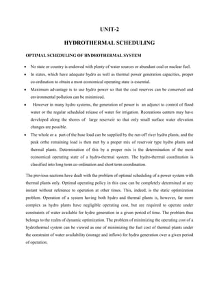
2. Fig. 2.1 Fundamental hydrothermal system
For the sake of simplicity and understanding, the problem formulation and solution technique are
illustrated through a simplified hydrothermal system of Fig. 2.1. This system consists of one
hydro and one thermal plant supplying power to a centralized load and is referred to as a
fundamental system. Optimization will be carried out with real power generation as control
variable, with transmission loss accounted for by the loss formula.
Mathematical Formulation
For a certain period of operation T (one year, one month or one day, depending upon the
requirement), it is assumed that (i) storage of hydro reservoir at the beginning and the end of the
period are specified, and (ii) water inflow to reservoir (after accounting for irrigation use) and
load demand on the system are known as functions of time with complete certainty (deterministic
case). The problem is to determine q(t), the water discharge (rate) so as to minimize the cost of
thermal generation.
𝐶𝑇 = 𝐶′
𝑃𝐺𝑇 𝑡 𝑑𝑡 (3.1)
𝑇
0
under the following constraints:
(i) Meeting the load demand
PGT(t) + PGH(t) – PL(t) – PD(t) = 0; t ε [0,T] (3.2)

3. This is called the power balance equation.
(ii) Water availability
𝑋′
𝑇 − 𝑋′
0 − 𝐽(𝑡)𝑑𝑡
𝑇
0
+ 𝑞(𝑡)𝑑𝑡
𝑇
0
= 0 (3.3)
where J(t) is the water inflow (rate), X'(t) water storage, and X’(0) , X’ (T) are specified water
storages at the beginning and at the end of the optimization interval.
(iii) The hydro generation PGH(t) is a function of hydro discharge and water storage (or head), i.e.
PGH(t) = f(X'(t),q(t)) (3.4)
The problem can be handled conveniently by discretization. The optimization interval T is
subdivided into M subintervals each of time length ΔT. Over each subinterval it is assumed that
all the variables remain fixed in value. The problem is now posed as
𝑚𝑖𝑛 ΔT C′
(PGT
m
)
M
m=1
= 𝑚𝑖𝑛 C(PGT
m
)
M
m=1
(3.5)
under the following constraints:
(i) Power balance equation
𝑃𝐺𝑇
𝑚
+ 𝑃𝐺𝐻
𝑚
– 𝑃𝐿
𝑚
– 𝑃𝐷
𝑚
= 0 (3.6)
where
𝑃𝐺𝑇
𝑚
= thermal generation in the mth interval
𝑃𝐺𝐻
𝑚
= hydro generation in the mth interval
𝑃𝐿
𝑚
=transmission loss in the mth interval
= 𝐵𝑇𝑇(𝑃𝐺𝑇
𝑚
)2
+ 2𝐵𝑇𝐻𝑃𝐺𝐻
𝑚
+ 𝐵𝐻𝐻(𝑃𝐺𝐻
𝑚
)2
𝑃𝐷
𝑚
= load demand in the mth interval
(ii) Water continuity equation

4. 𝑋′𝑚
− 𝑋′(𝑚−1)
− 𝐽𝑚
ΔT + 𝑞𝑚
ΔT = 0
where
X’m
= water storage at the end of the mth interval
Jm
= water inflow (rate) in the mth interval
qm
= water discharge (rate) in the mth interval
The above equation can be written as
𝑋𝑚
− 𝑋(𝑚−1)
− 𝐽𝑚
+ 𝑞𝑚
= 0; 𝑚 = 1,2, … . , 𝑀 (3.7)
where Xm
= X’m
/ΔT = storage in discharge units.
In Eqs. (3.7), Xo
and XM
are the specified storages at the beginning and end of the optimization
interval.
(iii) Hydro generation in any subinterval can be expressed as
𝑃𝐺𝐻
𝑚
= ℎ𝑜 1 + 0.5𝑒(𝑋𝑚
+ 𝑋𝑚−1
) 𝑞𝑚
− 𝜌 (3.8)
where
ho = 9.81 × 10-3
h’o
ho = basic water head (head corresponding to dead storage)
e = water head correction factor to account for head variation with storage
ρ = non-effective discharge (water discharge needed to run hydro generator at no load).
In the above problem formulation, it is convenient to choose water discharges in all subintervals
except one as independent variables, while hydro generations, thermal generations and water
storages in all subintervals are treated as dependent variables. The fact, that water discharge in
one of the subintervals is a dependent variable, is shown below:
Adding Eq. (3.7) for m = l, 2, ...,M leads to the following equation, known as water availability
equation

5. 𝑋𝑀
− 𝑋0
− 𝐽𝑚
𝑚
+ 𝑞𝑚
𝑚
= 0 (3.9)
Because of this equation, only (M - l) qs can be specified independently and the remaining one
can then be determined from this equation and is, therefore, a dependent variable. For
convenience, q1
is chosen as a dependent variable, for which we can write
𝑞1
= 𝑋0
− 𝑋𝑀
+ 𝐽𝑚
𝑚
− 𝑞𝑚
𝑀
𝑚=2
(3.10)
Solution Technique
The problem is solved here using non-linear programming technique in conjunction with the first
order gradient method. The Lagrangian is formulated by augmenting the cost function of Eq.
(3.5) with equality constraints of Eqs. (3.6)-(3.8) through Lagrange multipliers (dual variables)
𝜆1
𝑚
, 𝜆2
𝑚
𝑎𝑛𝑑 𝜆3
𝑚
. Thus,
ℒ = 𝐶 𝑃𝐺𝑇
𝑚
− 𝜆1
𝑚
𝑃𝐺𝑇
𝑚
+ 𝑃𝐺𝐻
𝑚
– 𝑃𝐿
𝑚
– 𝑃𝐷
𝑚
+ 𝜆2
𝑚
𝑋𝑚
− 𝑋 𝑚−1
− 𝐽𝑚
+ 𝑞𝑚
+
𝑚
𝜆3
𝑚
𝑃𝐺𝐻
𝑚
− ℎ𝑜 1 + 0.5𝑒(𝑋𝑚
+ 𝑋𝑚−1
) 𝑞𝑚
− 𝜌 (3.11)
The dual variables are obtained by equating to zero the partial derivatives of the Lagrangian with
respect to the dependent variables yielding the following equations
𝜕ℒ
𝜕𝑃𝐺𝑇
𝑚 =
𝑑𝐶(𝑃𝐺𝑇
𝑚
)
𝑑𝑃𝐺𝑇
𝑚 − 𝜆1
𝑚
1 −
𝜕𝑃𝐿
𝑚
𝜕𝑃
𝐺𝑇
𝑚 = 0 (3.12)
𝜕ℒ
𝜕𝑃
𝐺
𝑚 = 𝜆3
𝑚
− 𝜆1
𝑚
1 −
𝜕𝑃𝐿
𝑚
𝜕𝑃
𝐺𝐻
𝑚 = 0 (3.13)
𝜕ℒ
𝜕𝑋𝑚 𝑚≠𝑀
≠0
= 𝜆2
𝑚
− 𝜆2
𝑚+1
− 𝜆3
𝑚
0.5ℎ𝑜𝑒 𝑞𝑚
− 𝜌 − 𝜆3
𝑚+1
0.5ℎ𝑜𝑒 𝑞𝑚+1
− 𝜌 = 0 (3.14)
and using Eq. (3.7) in Eq. (3.11), we get

6. 𝜕ℒ
𝜕𝑞1
= 𝜆2
1
− 𝜆3
1
ℎ𝑜 1 + 0.5 𝑒 2𝑋0
+ 𝐽1
− 2𝑞1
+ 𝜌 = 0 (3.15)
The dual variables for any subinterval may be obtained as follows:
(i) Obtain 𝜆1
𝑚
from Eq. (3.12).
(ii) Obtain 𝜆3
𝑚
from Eq. (3.13).
(iii) Obtain 𝜆2
1
from Eq. (3.15) and other values of 𝜆2
𝑚
(𝑚 ≠ 1) from Eq. (3.14).
The gradient vector is given by the partial derivatives of the Lagrangian with respect to the
independent variables. Thus
𝜕ℒ
𝜕𝑞𝑚
𝑚≠1
= 𝜆2
𝑚
− 𝜆3
𝑚
ℎ𝑜 1 + 0.5 𝑒 2𝑋𝑚−1
+ 𝐽𝑚
− 2𝑞𝑚
+ 𝜌 (3.16)
For optimality the gradient vector should be zero if there are no inequality constraints on the
control variables.