
More Related Content
Similar to 3.pdf
Similar to 3.pdf (20)
Recently uploaded
Recently uploaded (20)
3.pdf
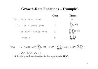
- 1. 63 Growth-Rate Functions – Example3 Cost Times for (i=1; i<=n; i++) c1 n+1 for (j=1; j<=i; j++) c2 for (k=1; k<=j; k++) c3 x=x+1; c4 T(n) = c1*(n+1) + c2*( ) + c3* ( ) + c4*( ) = a*n3 + b*n2 + c*n + d So, the growth-rate function for this algorithm is O(n3) = + n j j 1 ) 1 ( = = + n j j k k 1 1 ) 1 ( = = n j j k k 1 1 = + n j j 1 ) 1 ( = = + n j j k k 1 1 ) 1 ( = = n j j k k 1 1
- 2. 64 Orders of Algorithms Example: For k = 1 to n/2 do { …. } For j = 1 to n*n do { ---- } n/2 k=1 c + n*n j=1 c = c.n/2 + c.n2 = O (n2) Example: For k = 1 to n/2 do { For j = 1 to n*n do { ---- } } n/2 k=1 n*n j=1 c= c.n/2 *n2 = O(n3)
- 3. 65 Orders of Algorithms Example: i = n while i > 1 do { i = i div 2 } 64 32 16 8 4 2 1 O(log2n) Example: For i = 1 to n do For j = i to n do For k = i to j do m =m + i + j + k n i=1 n j=i j k=i3 n3/10 additions, that is O(n3) n i=1 n j=i 3(j-i +1) = n i=1[3 n j=i j - 3 n j=i i + 3 n j=i 1] = n i=1[3( n j=1 j - i-1 j=1 j) – 3i(n-i+1) + 3(n-i +1)] = n i=1[3[(n(n+1))/2 – (i(i-1))/2)] – 3i(n-i+1) + 3(n-i+1)] n3/10 additions, that is, O(n3)
- 4. 66 Growth-Rate Functions – Recursive Algorithms void hanoi(int n, char source, char dest, char spare) { Cost if (n > 0) { c1 hanoi(n-1, source, spare, dest); T(n-1) cout << "Move top disk from pole " << source c3 << " to pole " << dest << endl; hanoi(n-1, spare, dest, source); T(n-1) } } • The time-complexity function T(n) of a recursive algorithm is defined in terms of itself, and this is known as recurrence equation for T(n). • To find the growth-rate function for that recursive algorithm, we have to solve that recurrence relation.
- 5. 67 Growth-Rate Functions – Hanoi Towers • What is the cost of hanoi(n,’A’,’B’,’C’)? when n=0 T(0) = c1 when n>0 T(n) = c1 + T(n-1) + c3 + T(n-1) = 2*T(n-1) + (c1+c3) = 2*T(n-1) + c recurrence equation for the growth-rate function of hanoi-towers algorithm • We have to solve this recurrence equation to find the growth-rate function of hanoi-towers algorithm
- 6. 68 Recurrences There are four methods for solving recurrences, which is for obtaining asymptotic and O bounds on the solution. 1. The iteration method converts the recurrence into a summation and then relies on techniques for bounding summations to solve the recurrence. 2. In the substitution method, we guess a bound and then use mathematical induction to prove our guess correct. 3. The master method provides bounds for recurrences of the form T(n) = aT(n/b) + f(n) where a 1, b 2, and f(n) is a given function. 4. Using the characteristic equation.
- 7. 69 2 Solving recurrences by iteration method: converts the recurrence into a summation and then relies on techniques for bounding summations to solve the recurrence. Example: The recurrence arises for a recursive program that makes at least n number of disk moves from one peg to another peg and then move them to the third one. tn = 2tn-1 + 1, n 2, subject to t1 = 1. tn = 2tn-1 + 1 = 22tn-2 + 2 + 1 = ... = 2n-1t1 + 2n-2 + ... + 2 + 1 = 2n - 1. tn O(2n). This is the minumum number of moves required to transfer n disks from one peg to another. Indeed, before this move, we must first move all other disks to the third disk and also, after the move of the largest disk, we must move all other disks to the top of the largest disk. Therefore, the minimum number f(n) of moves satisfies the following inequality: f1 = 1 and fn 2fn-1 + 1, n 2. Thus, fn tn = 2n - 1 fn O(2n) For n = 64, it takes 584 * 106 years if every 1000 moves takes 1 seconds. Recurrences (cont.)
- 8. 70 2 Example: The recurrence arises for a recursive program that loops through the input to eliminate one item: tn = tn-1 + n n 2, subject to t1 = 1. To solve such a recurrence, we “telescope” it by applying it to itself, as follows: tn = tn-1 + n tn = tn-2 + (n-1) + n tn = tn-3 + (n-2) + (n-1) + n …… tn = t1 + 2+ … + (n-2) + (n-1) + n tn = 1 + 2+ … + (n-2) + (n-1) + n = n(n+1)/2 Hence, tn (n2/2) Recurrences (cont.)
- 9. 71 Example: The recurrence arises for a recursive program that has to make a linear pass through the input, before, during, or after it is split into two halves: tn = 2tn/2 + n n 2, subject to t1 = 0. To solve such a recurrence, we assume that n = 2k (k = lgn) and then “telescope” it by applying it to itself, as follows: tn = 2(2tn/4 + n/2) + n = 4tn/4 + 2n/2 + n = 4tn/4 + n (1+ 1) = 4(2tn/8 + n/4) + 2n/2 + n = 8tn/8 + 4n/4 + 2n/2+ n = 8tn/8 + n (1+ 1 + 1) …. = ntn/n + n(1+…+1) = 2kt1 + n.k tn = 0+ n(lgn) Hence, tn (nlgn) Recurrences (cont.)
- 10. 72 2 Solving recurrences by substitution (guess) method: Guesses a bound and then use mathematical induction to prove the guess correct. Example: The recurrence arises for a recursive program that halves the input in one step: tn = tn/2 + c n 2, subject to t1 = 1. t2 = 1 + c t4 = 1 + 2c, t8 = 1 + 3c, …. tn = 1 + kc, where n = 2k , tn = 1 + c.lgn, Therefore, tn (lgn) Proof by induction: Base case: n=1, t1 = 1 is given Induction case: n=k, tk = 1 + kc, where n = 2k , for tk = tk/2 + c, is true Proof: n=k+1, tk+1 = 1 + (k+1)c = 1+ kc + c ??? From the given recurrence (tk+1= T(2k+1) = T (2k+1/ 2)+c= T(2k)+c)= tk+c= 1+kc + c (by the induction step). Therefore, tn = 1 + c.lgn, for n = 2k Recurrences (cont.)
- 11. 73 Example: The recurrence arises for a recursive program that halves the input in one step, applies to 3 subproblems and loops through each input: tn = 3tn/2 + cn n 2, subject to t1 = 1. t2 = 3 + 2c t4 = 9 + 10c t8 = 27 + 38c t16 = 81 + 130c …. t2k = 3k + 2kc [(3/2)k –1] / [(3/2) –1], where n = 2k and k = lgn tn = 3lgn + cn(3lgn/n - 1) / 1/2 tn = n1.59 + 2cn (n0.59 – 1), where 3lgn = nlg3 = 31.59 = n1.59 (1 + 2c) – 2cn tn (n1.59) Recurrences (cont.)
- 12. 74 3 Solving recurrences by master method: The master method depends on the following theorem: Master theorem: Let a 1 and b 2 be constants and let T(n) be a function, and let T(n) be defined on the nonnegative integers by the recurrence T(n) = aT(n/b) + cni (n > n0), when n/ n0 is a power of b. Show that the exact order of T(n) is given by (nilogbn) case 1: a = bi, i =logba T(n) (nlogba) case 2: a > bi, i <logba (ni) case 3: a < bi, i >logba Example: The recurrence arises for a recursive program that halves the input, but perhaps must examine every item in the input: tn = tn/2 + n for n 2, subject to t1 = 0. For this recurrence, a = 1, b = 2, i = 1, and thus case 3: a < bi applies and tn (n) Example: The recurrence arises from matrix multiplication: tn = 8tn/2 + cn2 n 2, subject to t1 = 1. For this recurrence, a = 8, b = 2, i = 2, and thus case 3: a > bi applies and tn (nlog28) = (n3) Recurrences (cont.)
- 13. 75 Master Theorem (Another Version (text book): let a 1 and b>1 be constants, let f(n) be a function, and T(n) be defined on the nonnegative integers by the recurrence T(n) = aT(n/b) + f(n), a 1 and b > 1. The function divides the problem of size n into a subproblems, each of size n/b. The subproblems are solved recursively each in time T(n/b). The cost of dividing the problem and combining the results of the subproblems is described by the f(n). We interpret n/b to mean either n/b or n/b , which does not affect the asymptotic behaviour of the recurrence. T(n) can be bounded asymptotically as follows: 1. If f(n) = (nlogba - ) for some constant >0, then T(n)= (nlogba). 2. If f(n) = (nlogba ), then T(n) = (nlogbalgn). 3. If f(n) = (nlogba + ) for some constant >0, and af(n/b) cf(n) for some constant c < 1 and all sufficiently large n, then T(n) = (f(n)). Intuitively, the solution to the recurrence is determined by the larger of the two functions, f(n) and nlogba. In case 1, not only must f(n) be smaller than nlogba, it must be polynomially smaller. That is, f(n) must be asymptotically smaller than nlogba by a factor of n for some constant > 0. Similar technicality is valid for case 3, in addition satisfy the “regularity” condition that af(n/b) cf(n). Recurrences (cont.)
- 14. 76 The three cases do not cover all the possibilities for f(n). Example: The recurrence arises for a recursive program that divides the input into three and solves 9 of sub probles, and perhaps must examine every item in the input: tn = 9tn/3 + n, for n 3, subject to t1 = 1. Here a = 9, b = 3, f(n) = n and nlogba = nlog39 = (n2). Since f(n) = O (nlog39- ), where = 1, we can apply case 1 of the master theorem and conclude that the solution is tn (n2). Example: A recurrence arises from a search algorithm. tn = t2n/3 + 1, n 3, subject to t2 = 1. Here a = 1, b = 3/2, thus nlogba = nlog3/21= (n0) = 1, and f(n) = 1. Therefore, case 2 applies, since f(n)= (nlogba )= (1), and the solution to the recurrence is tn= (lgn). Recurrences (cont.)
- 15. 77 Example: The recurrence arises from a recursive algorithm. tn = 3tn/4 + nlgn, n 4, subject to t1 = 1. For this recurrence, a = 3, b = 4, and thus nlogba = nlog43 = O(n0.793), f(n) = nlgn. Since f(n) = (nlog43+ ), where 0.2, case 3 applies if we can show that the regularity condition holds for f(n). For sufficiently large n, af(n/b) = 3(n/4)lg(n/4) (3/4)nlgn = cf(n) for c = ¾ < 0. Consequently, by case 3, the solution to the recurrence is, tn (nlgn). Example: The master method does not apply the following recurrence. tn = 2tn/2 + nlgn. In this a = 2, b = 2, f(n) =nlgn, and nlogba = n. It seems that case 3 should apply, since f(n) = nlgn is asymptotically larger than nlogba = n but not polynomially larger. The ratio f(n)/nlogba = (nlgn)/n = lgn is asymptotically less than n for any positive constant . Consequently, the recurrence falls into the gap between case 2 and case 3. Therefore, the master method cannot be used to solve this recurrence. Recurrences (cont.)
- 16. 78 4 Solving Recurrences Using the Characteristic Equation • Homogeneous Recurrences: First we introduce homogeneous linear recurrences with constant coefficients, that is, recurrence of the form • a0tn + a1tn-1 + … + aktn-k = 0 (1) • where i. the ti are the values we are looking for. The recurrence is linear since it does not contain terms of the form titi+j, ti 2, and so on; ii. the coefficients ai are constants; and iii. the recurrence is homogeneous because the linear combination of the ti is equal to zero. • Example: Consider the familiar recurrence for the Fibonacci sequence. • fn = fn-1 + fn-2 which is fn - fn-1 - fn-2 = 0, • Therefore, Fibonacci sequence corresponds to a homogeneous linear recurrence with constants coefficients k = 2, a0 = 1 and a1 = a2 = -1. • It is interesting to note that any linear combination of solutions is itself a solution. Recurrences (cont.)
- 17. 79 • Trying to solve a few easy examples of recurrences of the form (1) by intelligent guesswork (or after a while intuition) may suggest we look for a solution of the form • tn = xn • where x is a constant as yet unknown. If we try this solution in (1), we obtain a0xn+ a1xn-1 +…+ akxn-k = 0 • This equation is satisfied if x = 0, a trivial solution of no interest. Otherwise, the equation is satisfied if and only if • a0xk+ a1xk-1 +…+ ak = 0. • This equation of degree k in x is called the characteristic equation of the recurrence of (1) and P(x) = a0xk+ a1xk-1 +…+ ak • is called its characteristic polynomial. • Recall that the fundamental theorem of algebra states that any polynomial p(x) of degree k has exactly k roots (not necessarily distinct), which means that it can be factorized as a product of k monomials • P(x) = 1 i k (x-ri) • where the ri may be complex numbers. Moreover, these ri are the only solutions of the equation p(x). Recurrences (cont.)
- 18. 80 Suppose that the k roots r1, r2, …, rk of this characteristic equation are all distinct. Since p(ri) = 0, it follows that x = ri is a solution to the characteristic equation and therefore ri n is a solution to the recurrence. Since any linear combination of solutions is also a solution, we conclude that the following satisfies the recurrence (1) for any choice of constants c1, c2, …, ck: tn = ciri n • of terms ri n is a solution of the recurrence (1), where the k constants c1, c2, …, ck are determined by the initial conditions. We need exactly k initial conditions to determine the values of these k constants. The remarkable fact, which we do not prove here, is that (1) has only solutions of this form. • Example: Consider the recurrence tn - 3tn-1 - 4tn-2 = 0 n 2, subject to t0 = 0, t1 = 1. • The characteristic equation of the recurrence is x2 - 3x - 4 = 0, whose roots are –1 and 4. The general solution therefore has the form tn = c1(-1)n +c24n. • The initial conditions give c1 +c2 = 0 n = 0, -c1 + 4c2 = 1 n = 1, that is, c1= -1/5, c2= 1/5 • We finally obtain tn = 1/5 [4n – (-1)n ], that is, tn (4n). Recurrences (cont.)
- 19. 81 Example: (Fibonacci) Consider the recurrence tn - tn-1 - tn-2 = 0 n 2, subject to t0 = 0, t1 = 1. The characteristic polynomial is P(x)= x2 -x - 1 = 0 Whose roots are (1+ 5)/2 and (1- 5)/2. The general solution is therefore of the form tn = c1((1+ 5)/2)n + c2((1- 5)/2 )n. The initial conditions give c1 + c2 = 0 n = 0, ((1+ 5)/2)c1 + ((1- 5)/2 )c2 = 1 n = 1, Solving these equations, we obtain c1= 1/ 5, c2= -1/ 5. We finally obtain tn = 1/ 5 [((1+ 5)/2) n – ((1- 5)/2) n ], which is de Moivre’s famous formula for the Fibonacci sequence. Therefore, tn ((1+ 5)/2) n. Recurrences (cont.)
- 20. 82 Now suppose that the roots of the characteristic equation are not all distinct. Then tn =nrn is also a solution of (1). That is, a0nrn + a1(n-1)rn-1+…+ ak(n-k)rn-k = 0, More generally, if m is the multiplicity of the root r, then tn = rn, tn = nrn, tn = n2rn, …, tn = nm-1rn are all possible solutions of (1). The general solution is a linear combination of these terms and of the terms contributed by the other roots of the characteristic equation. Once again there are k constants to be determined by the initial conditions. Example: Solve the following recurrence: tn = 5tn-1 - 8tn-2 + 4tn-3 n 3, subject to t0 = 0, t1 = 1, and t2 = 2. The characteristic equation is x3 - 5x2 + 8x - 4 = 0, or (x-1)(x-2)2 = 0. The roots are 1 and 2 (of multiplicity 2). The general solution is therefore tn = c11n +c22n +c3n2n. The initial conditions give c1 +c2 = 0 n = 0, c1 + 2c2 + 2c3 = 1 n = 1, c1 + 4c2 + 8c3 = 2 n = 2, From which we find c1 = -2, c2 = 2, c3 = -1/2. Therefore, tn = 2n +1- n2n-1 – 2 . tn (n2n). Recurrences (cont.)
- 21. 83 Inhomogeneous Recurrences: We now consider recurrences of a slightly more general form. a0tn + a1tn-1 + … + aktn-k = bnp(n) (2) The left hand side is the same as (1), but on the right hand side we have bnp(n), where b is a constant; an p(n) is a polynomial in n of degree d. Example: Solve the following recurrence: tn - 2tn-1 = 3n. In this case b =3 and p(n) = 1, a polynomial of degree d=0. A little manipulation allows us to reduce this example to the form (1). To see this, we first multiply the recurrence by 3, obtaining 3tn - 6tn-1 = 3n+1. If we replace n by n+1 in the original recurrence, we get tn+1 - 2tn = 3n+1. Finally, subtracting these two equations, we have tn+1 - 5tn + 6tn-1 = 0, which can be solved by the above method. The characteristic equation is x2 - 5x + 6 = 0. That is, (x-2)(x-3) = 0. Intuitively we can see that the factor (x-2) corresponds to the left-hand side of the original recurrence, whereas the factor (x-3) has appeared as a result of our manipulation to get rid of the right-hand side. Recurrences (cont.)
- 22. 84 Generalizing this approach, we can show that to solve (2) it is sufficient to take the following characteristic equation (a0xk+ a1xk-1 +…+ ak )(x-b)d+1 = 0. Once this equation is obtained, proceed as in the homogeneous case. Example: The number of movements of a ring required in the Towers of Hanoi problem is given by the following recurrence relation: tn = 2tn-1 + 1, n 1, subject to t0 = 0. The recurrence can be written tn - 2tn-1 = 1, which is of the form (2) with b = 1, p(n) = 1, a polynomial of degree 0. The characteristic equation is therefore (x-2)(x-1) = 0. The roots of this equation are 1 and 2, so the general solution of the recurrence is tn = c11n +c22n. We need two initial conditions. We know that t0 = 0; to find a second initial condition we use the recurrence itself to calculate t1 = 2t0 +1 = 1. We finally have c1 +c2 = 0 n = 0 c1 + 2c2 = 1 n = 1 From which we obtain the solution, tn = 2n –1, where c1= -1, c2 = 1. Then we can conclude that tn (2n). Recurrences (cont.)
- 23. 85 A further generalization of the same type of argument allows us finally to solve recurrences of the form a0tn + a1tn-1 + … + aktn-k = b1 np1(n) + b2 np2(n)+… (3) where the bi are distinct constants and pi(n) are polynomials in n respectively of degree di. It suffices to write the characteristic equation (a0xk+ a1xk-1 +…+ ak )(x- b1)d1+1(x- b2)d2+1 … = 0, Example: Solve the following recurrence: tn = 2tn-1 + n + 2n n 1, subject to t0 = 0. tn - 2tn-1 = n + 2n, which is of the form (3) with b1=1, p1(n) = n, b2 =2, p2(n) = 1. The characteristic equation is (x-2)(x-1)2(x-2) = 0, Roots: 1, 2, 2. The general solution of the recurrence is therefore of the form tn = c11n + c2n1n + c32n + c4n2n Using the recurrence, we can calculate t1= 3 (t1= 0+1+21 = 3), t2 = 12, t3 = 35. c1 +c3 = 0 n = 0, c1 + c2 + 2c3 + 2c4 = 3 n = 1 c1 + 2c2 + 4c3 + 8c4 = 12 n = 2 c1 + 3c2 + 8c3 + 24c4 = 35 n = 3, arriving at tn = -2 – n + 2n+1 + n2n Therefore, tn (n2n). Recurrences (cont.)
- 24. 86 Change of Variable: • We write T(n) for the term of a general recurrence, and tk for the term of a new recurrence obtained by a change of variable. Example: Solve the recurrence if n is a power of 2 and if T(n) = 4T(n/2) + n n > 1. Replace n by 2k (so that k = lgn) to obtain T(2k) = 4T(2k-1) + 2k. This can be written as tk = 4tk-1 + 2k if tk = T(2k) = T(n). We know how to solve this new recurrence: the characteristic equation is (x-4)(x-2) = 0 and hence tk = c14k + c22k. Putting n back instead of k, we find T(n) = c1n2 + c2n. T(n) is therefore in O(n2 | n is a power of 2). Recurrences (cont.)
- 25. 87 Example: Solve the recurrence if n is a power of 2 and if T(n) = 2T(n/2) + nlgn n > 1. Replace n by 2k (so that k = lgn) to obtain T(2k) = 2T(2k-1) + k2k. This can be written as tk = 2tk-1 + k2k if tk = T(2k) = T(n). We know how to solve this new recurrence: the characteristic equation is (x-2)3 = 0, (since tk - 2tk-1 = k2k, where b = 2, p(k) = k, and d = 1), and hence tk = c12k + c2k2k + c3k22k. Putting n back instead of k, we find T(n) = c1n + c2nlgn + c3nlg2n. Hence T(n) O(nlg2n | n is a power of 2). Example: Solve the recurrence if n is a power of 2 and if T(n) = 3T(n/2) + cn (c is constant, n = 2k > 1.) Replace n by 2k (so that k = lgn) to obtain T(2k) = 3T(2k-1) + c2k. This can be written as tk = 3tk-1 + c2k if tk = T(2k) = T(n). The characteristic equation is (x-3)(x-2) = 0, (since tk -3tk-1 = c2k, where b = 2, p(k) = c, and d = 0), and hence tk = c13k + c22k If we put n back, instead of k, we find T(n) = c13lgn + c2n. Since algb = blga, therefore, T(n) = c1nlg3 + c2n. Hence, T(n) O(nlg3). Recurrences (cont.)