2. Journal of Petroleum Science and Engineering 198 (2021) 108127
2
Furthermore, the ESP can operate in vertical, horizontal or deviated
wells, in onshore or offshore applications, lifting viscous fluids with a
determined quantity of gas and solids (Takács, 2017).
In the conventional ESP assembly, with the pump submersed at the
production well bottom, the main advantages are the performance and
operational stability of the pump, since the temperature and pressure in
the pump intake are the highest possible. The oil viscosity and the Gas
Void Fraction (GVF) are lower and the pump operates more efficiently.
The main disadvantage of ESP systems is their reliability issues.
Repairing an ESP positioned at the well bottom incurs extremely high
costs. When the pump or any system component fails, such as seal,
electric motor and connections, it is necessary to interrupt the produc
tion, remove the ESP system and replace. For wet completion wells, a
dedicated workover rig is required. Usually, this rig is leased at a high
cost and is limited within the supply chain.
Given the high maintenance cost of the ESPs, affordable alternatives
have been developed, such as boosting systems. In this context, an
important innovation is the Subsea Boosting ESP (SB-ESP) presented
initially by Rodrigues et al. (2005). The SB-ESP is a subsea boosting
technology where the motor/pump set is assembled on a capsule, which
in turn is positioned in a frame on the seabed outside of the producer
well. The main advantage of the SB-ESP system is its flexibility in
maintenance operations. The system can be installed by cables, which
dispenses high cost rigs. However, a disadvantage of the SB-ESP is the
pump’s performance and its operational stability. The oil reaches the
pump intake cooler and with lower pressure compared to the conven
tional installation within the producer well. The oil viscosity and the
GVF can increase, thus hindering the performance of the pump. More
recently, the SB-ESP technology was discussed by Colodette el at.
(2007), Teixeira et al. (2012), Costa et al. (2013), Tarcha et al. (2015)
and Tarcha et al. (2016).
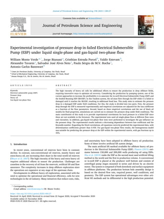
The motivation of this work involves the analysis of a combined
production layout using a pumping system, shown in Fig. 1, to increase
the production profitability of offshore heavy oil. This innovative layout
includes a conventional ESP and a SB-ESP placed in series. The ESP is
installed conventionally at the producer well bottom, while the SB-ESP
is positioned on the seabed, upstream of the Wet Christmas Tree.
In this layout, the wells were completed with sand, control screens,
and gravel packed throughout the nearly 800 m horizontal section in the
reservoir. A slant section of 80 m was built just before reaching the
reservoir for the ESP installation. The well completion has no flow
bypass in the ESP (Rocha et al., 2020).
The production system is initially operated by the downhole ESP
until a breakdown occurs, at which time the SB-ESP is put into
Nomenclature
A Area (m2
)
C1, C2 Empirical constants (− )
cp Specific heat (J/kg. K)
Di Inner diameter of the impeller (m)
Dh characteristic length of the impeller (m)
Do Outer diameter of the impeller (m)
g Gravity (m/s2
)
H Head loss (m)
K1,K∞,Ki,Kd Empirical constants (− )
K Loss coefficient (− )
m Empirical constants (− )
ṁ Mass flow rate (Kg/s)
n Number of stages (− )
P Gage pressure (Pa)
Pb Bubble pressure (Pa)
Q Volumetric flow rate (m3
/s)
q̇ Dissipated heat (Watts)
Re Reynolds Number (− )
R2
determination coefficient (− )
T Temperature (◦
C)
U Velocity profile (m/s)
U Relative uncertainty (%)
V Average velocity (m/s)
y Coordinate in direction of gravity (m)
А no-slip gas void fraction (− )
ΔH Enthalpy Increment rate (Watts)
ΔT Temperature increment (◦
C)
ΔP Pressure Loss (Pa)
ΔP Average pressure drop (− )
ξstd Standard deviation (− )
μ Dynamic viscosity (Pa.s)
ρ Density (kg/m3
)
ϕ correction factor of the kinetic energy (− )
Sub index
in At the inlet section of the stage
out At the outlet section of the stage
N At the stage number n
L Liquid phase
G Gas Phase
Fig. 1. Layout of subsea production system.
W. Monte Verde et al.
3. Journal of Petroleum Science and Engineering 198 (2021) 108127
3
operation. The advantage of this layout is the uninterrupted production
while the workover rig is awaited, since the SB-ESP can operate as
backup until the intervention in the well. Since the two systems are
assembled in series, the oil will have to flow through the failed down
hole ESP until it reaches the SB-ESP. It is clear that the damaged
downhole ESP will offer resistance to the fluid flow, which results in
pressure loss. The local pressure loss changes the system’s curve and
causes a decrease in the produced oil flowrate. In addition, the ESP
pressure drop can increase the GVF at the SB-ESP intake, impairing its
performance. This clarifies the need estimate the downhole ESP pressure
loss depending on the operating conditions.
The Tandem system described above with conventional ESP and a
SB-ESP is innovative. However, there are other studies in the literature
that report the application of a conventional ESP in Tandem with a
subsea multiphase boosting, using helicoaxial pumps, as reported by
Grimstad (2004).
Other researchers such as Hwang and Pal (1997), Azzi et al. (2000),
Jeong and Shah (2004), Roul and Dash (2009), Calçada et al. (2012),
Alimonti (2014), Pietrza and Witczak (2015), Colombo et al. (2015) and
Hendrix et al. (2017) have studied the pressure drop in fittings used in
the oil industry. These works are applied to valves, elbows, tools joints,
pigs, expansions and contractions; however, studies on the pressure loss
in a failed ESP are not reported in the literature.
This work aims to estimate the pressure drop in a damaged ESP under
field conditions. For this purpose, the study is divided into two parts.
First, the pressure drop through the ESP is measured experimentally and
empirical correlations are adjusted for the loss coefficient as a function
of the flow parameters. Second, based on these empirical correlations
and the use of black oil model for oil properties, simulations estimate the
pressure drop under field conditions.
The main contribution of this study is to provide experimental cor
relations for local pressure drop that enable the system curve calculation
and production system simulation. These results are essential for eval
uating the feasibility of the production layout studied.
For this purpose, an experimental setup was used to measure the
pressure drop in a damaged ESP. The ESP model tested is the same
equipment selected to operate in the Atlanta field wells, located at the
Santos Basin, offshore, Southeast Brazil, which produces heavy oil with
an API gravity of 14◦
.
The tests were carried out with oil single-phase flow at different flow
rates and viscosities. In addition, gas-liquid two-phase flow tests inves
tigated the gas influence on the pressure drop. Based on the proposed
experimental correlations, production layout analyses are performed
assuming black oil properties and different approaches.
2. The experimental setup
Given the lack of references in the literature, this study considers the
pressure drop through the ESP to be a minor or local loss, as is for fit
tings, such as valves, elbows, tools joints, expansions/contractions. Such
an approach consists of experimentally measuring the pressure drop in
the fitting on a full scale and then adjusting correlations for the head
loss.
The experimental study was conducted in the Experimental Labo
ratory of Petroleum – LabPetro, at the University of Campinas – UNI
CAMP. The experimental facility was especially designed to measure the
ESP’s performance with ultra-heavy oil. However, in this study, the fa
cility was used to investigate the pressure drop that occurs when the
fluid flows through a damaged ESP, either for liquid single-phase or gas-
liquid two-phase flow.
The ESP loop test is shown schematically in Fig. 2 and in a real aerial
view in Fig. 3. The experimental facility comprises an oil tank, a two-
screw booster pump, a temperature control system, an ESP, Variable
Speed Drives (VSDs), valves, measuring instrumentations and a power
generator.
The booster, with nominal flow rate of 200 m3
/h and pressure
increment of 25 bar, pumps the oil from the tank through the pipes up to
the ESP intake. This pump is driven by a VSD for rotational speed con
trol. Because it is a closed loop, the oil tends to heat up during the tests so
a temperature control system composed of a thermo-chiller and a heat
exchanger, with a 230,000 kCal/h capacity, is used to keep the fluid
temperature constant. This system is crucial because the viscosity is
controlled by the oil’s temperature.
Before the ESP intake, the oil mass flow rate is measured using a
Coriolis meter, series CMF 400 M, manufactured by Emerson Micro
Motion®. This sensor has a maximum range of 545,000 kg/h and an
Fig. 2. Schematic diagram of the ESP loop test. 1 - oil tank, 2 - booster pump, 3 - heat exchanger, 4 - cold water tank, 5 - heater, 6 - chiller, 7 - compressor, 8 -
nitrogen tank and 9 - ESP.
W. Monte Verde et al.
4. Journal of Petroleum Science and Engineering 198 (2021) 108127
4
accuracy of 0.1%. This instrument is also capable of measuring the
density with an accuracy of 0.5 kg/m3
.
For gas-liquid two-phase tests, nitrogen (N2) was used. For this, at
mospheric air is compressed, then runs through a nitrogen separation
plant and is mixed with the oil in the ESP intake. The nitrogen flow rate
is also measured with a series CMF 010 M Coriolis meter manufactured
by Emerson Micro Motion®, with 30 kg/h of maximum range and an
accuracy of 0.25%. After flowing through the damaged ESP, the mixture
flows return to the tank where the gas is gravitationally separated and
released.
The 10-stage ESP is driven by an electric motor and controlled by a
VSD. However, for this study, the pump is kept off. Pressure and tem
perature sensors are also installed in the ESP. The gage pressure and
temperature are measured at the pump intake and discharge. In addi
tion, differential pressure transducers are installed in each stage of the
ESP to analyze the pressure drop throughout the equipment. The tem
perature at the outlet of stages 3, 5, 7, and 9 are also measured.
Capacitive transducers (series 2051) manufactured by Rosemount®
were used to measure the differential pressure. The pressure sensors
have an accuracy of 0.05%. The temperature was measured with a
resistance temperature detector, type PT100, 1/10 DIN, with standard
accuracy. All instruments were connected to a data acquisition system,
manufactured by National Instruments®, which monitors, controls, and
stores data.
The ESP model used in the experimental facility is the same one
selected to operate in the wells of the Atlanta oil field, but with less
stages. Operating with water at 3500 rpm, the ESP HC20000L, 675 series
provides, at the best efficient point, a flow rate of 115 m3
/h (~17,360
BPD) and head per stage of 22.3 m. This ESP is manufactured by Baker-
Hughes®. The experimental facility is powered by an electric generator
with capacity of 750 kVA.
3. Research methodology
The research methodology aims to measure the head loss in the
damaged ESP under different operational conditions, such as gas and
liquid flow rate and viscosity. For this, a representative experimental
matrix was performed for the oil field conditions.
3.1. Liquid single-phase flow
The liquid single-phase flow tests were performed with crude dead
oil from the Atlanta field. Because the dead oil is highly viscous, it was
necessary to blend it using diesel fuel in order to obtain the field vis
cosity range. The oil/diesel blend properties, such as viscosity, density,
surface tension and specific heat, were then measured. In addition, the
blend rheology was characterized, evidencing its Newtonian behavior.
The temperature dependence of viscosity and density are shown in
Fig. 4. For simplicity, the crude dead oil/diesel blend is simply called
‘oil’.
The experimental procedure provides a certain oil flow rate in the
loop while the temperature is kept constant. The oil flow rate is
controlled by the rotational speed of the booster pump. Once the steady
state is established, all measured variables are captured, including the
pressure drop across the turned-off ESP. Then, the booster rotational
speed is changed, thus increasing the oil flow rate at constant temper
ature. Once the full range of oil flow rate is tested, a new temperature is
set and the procedure is repeated.
Oil flow through the damaged ESP may induce rotation in the
equipment. Thus, the liquid single-phase tests were performed in two
different configurations. In the first, the ESP shaft was left free, allowing
the induction of rotation by the oil flow. In the second, the pump shaft
was locked, which prevented any rotation. According to Alhanati et al.
(2001) this is a characteristic mechanical failure of ESPs described as
“stuck shaft”. The tests in these two configurations aim to represent the
possible failures in the field, rendering a more realistic estimate of head
loss.
The liquid single-phase experimental matrix covers an oil flow rate
range from 11,500 to 65,000 kg/h and viscosities of 130 to 1600 mPa s.
3.2. Gas-liquid two-phase flow
The two-phase flow tests were performed with oil as liquid phase and
nitrogen as gas phase. The crude oil is the same one used in the liquid
single-phase tests, characterized in Fig. 4. Nitrogen gas was selected for
safety reasons. For the pressure and temperature range, the nitrogen
compressibility factor is unitary, and its behavior is described as ideal
gas.
The oil/nitrogen surface tension and the blend’s specific heat used in
the tests are approximately constant and in the temperature range of
25–50 ◦
C; these are equal to 30.5 mN/m and 1.69 kJ/kg.K, respectively.
The experimental procedure provides a certain oil flow rate in the
loop while the temperature is kept constant. Then, the gas is injected and
mixed into the oil stream. Once the steady state is established, the data is
acquired. Thereafter, the gas flow rate is increased and a new opera
tional condition is reached. After testing all gas flow rate ranges, the oil
flow rate is increased at constant temperature. The gas flow rate range is
repeated for this new oil flow rate. This procedure is repeated until the
entire oil flow rate range is tested. Once this is done, a new temperature
is set and the procedure is repeated.
The two-phase experimental matrix covers an oil flow rate range
Fig. 3. ESP loop test.
Fig. 4. Temperature dependence of oil viscosity and density.
W. Monte Verde et al.
5. Journal of Petroleum Science and Engineering 198 (2021) 108127
5
from 14,200 to 49,500 kg/h, a gas flow rate from 0.4 to 12.9 kg/h, and
liquid viscosity between 195 and 830 mPa s, providing no-slip GVF of up
to 35%.
4. Mathematical modeling
This section presents the methodologies for reducing experimental
data and adjusting the empirical correlations for head loss. Additionally,
the approaches adopted to simulate pressure drop under oil field con
ditions are also shown.
4.1. Experimental data modeling
For the pump intake pressure greater than the oil saturation pressure
and negligible water cut, a liquid single-phase flow will occur. In this
case, the head loss through each stage of the failed ESP can be obtained
by a control volume analysis.
Considering steady-state, incompressible, isothermal, and one-
dimensional flow between the inlet (in) and outlet (out) sections of the
pump stage, as shown in Fig. 5, the integral energy equation becomes:
(
P
ρg
+ ϕ
V
2
2g
+ y
)
in
−
(
P
ρg
+ ϕ
V
2
2g
+ y
)
out
= Hn (1)
with
ϕ =
1
A
∫ (
U
V
)3
dA (2)
where P is the pressure, ρ is the liquid density, g is the acceleration of
gravity, Vis the liquid average velocity, y is the coordinate in direction of
gravity, Hn is the head loss in the stage n, U is the velocity component
and ϕ is the correction factor of the kinetic energy that takes into ac
count how U is distributed over the cross section A.
From Eq. (1) it is clear that Hn corresponds to the pressure drop when
(ϕV
2
)in = (ϕV
2
)out and yin = yout, that is when the flow is neither
accelerated nor decelerated and when the flow is horizontal, so that
there is no change in potential energy. Then, the pressure drop across the
stage n is written as:
Hn =
Pin − Pout
ρg
(3)
The flow regime through a device is quite complex and the theory is
very weak. The local losses are often measured experimentally and
correlated with the flow parameters in tubes. The measured local loss is
usually given as a ratio of the head loss through the device to the velocity
head, so the loss coefficient (K) is:
K =
Hn
V
2
2g
=
ΔPn
1
2
ρV
2
(4)
where Vis the fluid reference velocity, considered equal to the inlet
average velocity (Vin), defined by:
V = Vin =
4Q
π
(
D2
o − D2
i
) (5)
Fig. 5. Control Volume for the ESP stage.
W. Monte Verde et al.
6. Journal of Petroleum Science and Engineering 198 (2021) 108127
6
where Do and Di are outer and inner diameters of the impeller inlet,
respectively, as shown in Fig. 5; and Q is the volumetric liquid flow rate
given in the inlet conditions.
For the failed ESP, the experimental loss coefficient (K) can be
calculated by measuring the pressure drop across the stage (ΔPn) and the
flow rate in order to calculate the reference velocity (V). Usually, the
local head loss coefficient, given by Eq. (4), is correlated with the Rey
nolds number (Re), defined by:
Re =
ρVDh
μ
(6)
where μ is the liquid dynamic viscosity and Dh is the characteristic
length.
In the present work, the characteristic length (Dh) is defined as the
difference between the outer (Do) and inner (Di) diameters of the
impeller inlet. This characteristic length definition is equivalent to the
hydraulic diameter of an annular tube with the same dimensions as the
impeller inlet. As the pump stages are assembled in series, the hydraulic
diameters of the impeller inlet and the diffuser outlet must be concor
dant and equal, corroborating the hypothesis of neglecting the kinetic
terms of Eq. (1). Although there is no consensus in the literature, this
definition of characteristic length for pumps has been used by other
authors, such as Stel et al. (2015) and Ofuchi et al. (2017). For the ESP
model used, the outer and inner diameters are 80.2 mm and 38.1 mm,
respectively.
So far, no consideration has been made about the flow regime, which
is when the flow is laminar or turbulent. In general, for fully turbulent
flow in fittings, the K coefficient is tabulated and independent of the
Reynolds number. However, for laminar flow, K is dependent on the
Reynolds number (Coker, 2007). Since there are no studies in the
literature reporting the head loss in ESPs, it is necessary to investigate
when K is a constant value or not. In a dimensionless theory, this cor
responds to the question of how K depends on the Reynolds number.
Based on the literature review, different proposals are found to adjust
the K-dependence of the Reynolds number. In this work, equations
traditionally used to correlate this dependence were tested to verify
which one best represents the experimental data. The equations pro
posed by Kittredge and Rowley (1957), Churchill and Usagi (1974),
Hooper (1981) and Darby (2001) were considered.
Kittredge and Rowley (1957) suggested a power law equation given
by:
K = C1Re− C2
(7)
where C1 and C2 are constants of the experimental adjustment.
Churchill and Usagi (1974) proposed a standardized procedure to
produce correlations in the form of a common empirical equation. This
equation is given by:
K =
[
Cm
1 +
(
C2
Re
)m]1/m
(8)
where C1, C2 and m are constants of the experimental adjustment for a
specific fitting.
Hooper (1981) developed another traditional approach known as the
2-K method. This method is independent of the roughness of the fittings
but is a function of the Reynolds number and fitting diameter (D). Giving
the diameter in millimeters, this method is expressed as:
K =
K1
Re
+ K∞
(
1 +
25.4
D
)
(9)
where K1 and K∞ are constants of the experimental adjustment. The
physical meaning becomes obvious in the Reynolds number limits: K ≈
K1 for the fitting at Re→1 (laminar flow) and K≈K∞ for a large fitting at
Re→∞ (turbulent flow).
Darby (2001) proposed an approach known as the 3-K method in an
attempt to improve the prediction accuracy of the head loss for a system
with large fittings. This method is a function of the Reynolds number,
fitting diameter and three K-constants. Providing the diameter in mil
limeters, this method is expressed as:
K =
K1
Re
+ Ki
[
1 + Kd
(
25.4
D
)0.3]
(10)
where K1, Ki and Kd are constants of the experimental adjustment.
Both correlations of Hooper (1981) and Darby (2001) require the
fitting diameter D. For ESP, the fitting diameter D was considered equal
to the characteristic diameter Dh, as defined previously.
4.2. Pressure drop simulations through the ESP under field conditions
Once the empirical correlation between the loss coefficient and the
flow parameters is adjusted, it is possible to simulate the estimated
pressure drop through the ESP under oil field conditions, such as an ESP
with more stages and higher pressures and temperatures. Due to the
fluid complexity and the uncertainties regarding their properties in
downhole conditions, it is necessary to simplify assumptions to enable
these simulations.
The pressure drop (ΔP) in a failed n-stage ESP can be calculated as a
sum of the loss at each stage:
ΔP =
∑
n
i=1
ΔPn =
∑
n
i=1
(
1
2
KρV
2
)
(11)
where the fluid properties and flow conditions are defined at the inlet of
each stage.
4.2.1. Liquid single-phase modeling
To estimate the pressure drop through the failed ESP under liquid
single-phase flow, non-isothermal flow was assumed. In this case, we
considered that all the energy dissipated as head loss is converted into
heat. This energy heats the fluid and there is no dissipation to the
external environment, that is, the adiabatic flow hypothesis is
considered.
Flowing through each stage of the pump, the fluid undergoes a
decrease in pressure and, consequently, an increase in temperature,
resulting in variations of density and oil viscosity. The continuous
heating of the fluid reduces the stage pressure drop and the head loss in
the last stages is lower than in the first ones. The change of the Reynolds
number along the pump requires a marching stage-by-stage algorithm to
calculate the fluid properties and the pressure loss at each stage, as
shown in Fig. 6.
For a simplified approach, we assume that because of the head loss,
the dissipated power (q̇n) at the pump stage n is given by:
q̇n = ΔPn Q (12)
As the flow is considered non-isothermal and adiabatic, all dissipated
power is converted to heating the fluid. The dissipated power is equal to
the enthalpy increment (ΔH):
q̇n = ΔH (13)
For incompressible fluid, the enthalpy increment is a function of
temperature. The fluid heating (ΔTn) is given by:
ΔTn =
q̇n
ṁ cP
(14)
where cp is the specific heat and ṁis the mass liquid flow rate.
From the data at the pump inlet, the procedure consists of calculating
the pressure loss in the first stage and then the temperature increase.
Once the black oil model is defined, it is possible to correct the fluid
properties at the outlet of the first stage and calculate a new Reynolds
W. Monte Verde et al.
7. Journal of Petroleum Science and Engineering 198 (2021) 108127
7
number. Then, the head loss at the second stage is calculated, the tem
perature increases, the fluid properties are corrected and the Reynolds
number is recalculated. This procedure is repeated continuously through
the last stage of the pump. By calculating the sum of the head loss of each
stage, the total ESP pressure loss is obtained.
The non-isothermal approach is suitable for ESPs with many stages
and heavy oils, where the heating effect becomes significant. It is also
necessary to ensure that the pressure is higher than the oil saturation
pressure. Otherwise, there will be continuous gas release along the
pump and another approach must then be used.
4.2.2. Two-phase modeling – homogeneous No-Slip model
If the ESP intake pressure is lower than the oil saturation pressure, or
bubble pressure (Pb), the lighter fractions of hydrocarbons evaporate
and gas-liquid two-phase flow occurs. Generally, the rigorous solutions
of the conservation’s equations for the gas-liquid two-phase are complex
and unavailable.
A feasible approach for two-phase flow is to consider earlier models,
which treat the system as single-phase flow. The Homogeneous No-Slip
approach is an earlier model that treats the two-phase mixture as a
pseudo single-phase fluid with average and fluid properties. The mixture
fluid properties are determined from the single-phase gas and liquid
properties, which are averaged on the basis of the no-slip liquid holdup
(Shoham, 2006).
Assuming steady-state one-dimensional flow, no slippage between
the phases, and that the phases are well-mixed and in equilibrium, the
average velocity and the average fluid properties can be calculated. The
gas-liquid mixture average velocity at the stage inlet is given by:
V =
QL + QG
A
(15)
where QL and QG are the volumetric flow rate of the liquid and gas
phases, respectively, at the inlet stage conditions.
The mixture density is calculated as a weighting between phases
properties:
ρ = αρG + (1 − α)ρL (16)
where ρL and ρG are the density of liquid and gas phases, respectively,
and α is the no-slip gas void fraction at the stage inlet, given by:
α =
QG
QG + QL
(17)
The mixture’s kinematic viscosity is considered equal to the kine
matic viscosity of the liquid phase. Thus, the mixture dynamic viscosity
can be calculated by:
μ = μL
(
ρ
ρL
)
(18)
where μL is the dynamic viscosity of the liquid phase.
The mixture Reynolds number is calculated by Eq. (6) based on the
mixture characteristics, where V, ρ and μ are given by Eqs. (15), (16) and
(18), respectively.
The pressure drop (ΔPn) in the stage n of the failed ESP under gas-
liquid two-phase flow, assuming homogeneous no-slip model, is calcu
lated by Eq. (4). If the homogeneous model is suitable, the empirical
correlations for K, as a Re-function adjusted for single-phase flow, can
also be used for gas-liquid flow using the properties of a pseudo fluid.
For a multi-stage ESP, the pressure drop across the pump (ΔP) is
calculated by Eq. (11).
Due to the decrease in pressure and the increase in temperature along
the ESP the free gas expansion and the gas release occurs due to the
decreased solubility ratio, causing an increase in the no-slip gas void
fraction, changing the mixture properties. Therefore, the mixture Rey
nolds number is not constant along the ESP stages, requiring a marching
stage-by-stage algorithm. The calculation procedure is similar to that
described for single-phase flow. However, the gas fraction must be
calculated stage by stage in order to define the properties of the mixture.
Therefore, from the data at the pump inlet, the procedure consists of
calculating the pressure loss and the heat dissipation in the first stage
and then its outlet pressure and temperature. The first stage outlet
conditions are the same as the inlet conditions of the next stage. Once
the second stage inlet conditions are known, the black oil model pro
vides the properties of the liquid and gas phases, the no-slip gas void
fraction and mixture properties can be calculated using the homogenous
model. Then, the head loss at the second stage is calculated. This pro
cedure is repeated continuously until the final stage of the pump. By
calculating the sum of the head loss of each stage, the total ESP pressure
loss is obtained.
Fig. 7 shows the flowchart for calculating pressure loss in ESP for
both single-phase and two-phase flow. This marching stage-by-stage
algorithm has an explicit calculation procedure. In general, the accu
racy of the homogeneous model is limited to the flow of small bubbles
dispersed in a continuous liquid phase, which is common in mixtures
with high liquid flow rates. In this study, the application range of the
homogeneous model for pressure drop calculation is experimentally
determined.
5. Experimental results
In this section, the results of the experimental pressure drop in the
failed ESP are shown and discussed. Initially, the results for single-phase
are presented and the measured data are fitted by empirical correlations.
In the sequence, the two-phase flow results are presented and, using the
homogeneous mixture model, comparisons of these data are drawn to
the adjusted correlations.
5.1. Liquid single-phase flow
Fig. 8 shows the pressure drop measured at each ESP stage under
different flow conditions. The continuous lines also indicate the average
pressure drop (ΔPn) for each operational condition, that is, the pressure
drop calculated by the total head loss divided by the number of ESP
stages.
These results indicate that the head losses at each stage vary slightly
around an average value. This trend is observed for the entire test matrix
Fig. 6. Marching stage-by-stage procedure to calculate the pressure drop through the failed ESP.
W. Monte Verde et al.
8. Journal of Petroleum Science and Engineering 198 (2021) 108127
8
with single-phase flow. This is expected given the properties of the dead
oil used as a working fluid.
The low compressibility and the reduced temperature variation
along the ESP do not promote significant variations in the fluid prop
erties, making the Reynolds number constant throughout the pump,
resulting in similar pressure drop for all stages.
Therefore, for reducing the experimental single-phase flow results,
an average loss coefficient approach was considered instead of calcu
lating a coefficient for each stage. The average loss coefficient is related
to the average pressure drop by (ΔPn):
K =
ΔPn
1
2
ρV
2
=
∑
n
i=1
ΔPn
n 1
2
ρV
2
(19)
Since the ESP model tested is the same used in the Atlanta field, the
geometric similarity is guaranteed. So that the experimental correlations
are suitable in the field conditions, it is necessary to base the analyses on
dimensionless numbers. Therefore, the average loss coefficient is pre
sented and correlated with the Reynolds number.
5.1.1. Free shaft tests
Fig. 9 shows the experimental results for oil single-phase flow and
presents the average loss coefficients as a function of the Reynolds
number in the free shaft tests. This figure also presents the fitted cor
relations between the loss coefficient and the Reynolds number pro
posed by Kittredge and Rowley (1957), Churchill and Usagi (1974),
Hooper (1981), and Darby (2001). The adjusted correlations and the
determination coefficients of the fit for each one are shown in Table 1.
The analysis of the experimental uncertainties is presented in Appendix
A.
The results show the decreasing dependence between K and Re. The
mean loss coefficient decreases as the Reynolds number increases.
Therefore, as the inertial forces increase, the loss coefficient decreases
with an asymptotic behavior and tends to be constant and independent
of the Reynolds number.
Regarding the fitted correlations shown in Table 1, we observe that
all equations properly represent the experimental data, with determi
nation coefficients (R2
) greater than 0.97. The correlation proposed by
Fig. 7. Flowchart to calculate the pressure drop through the ESP.
Fig. 8. Pressure drop measured at each pump stage under different
flow conditions.
W. Monte Verde et al.
9. Journal of Petroleum Science and Engineering 198 (2021) 108127
9
Churchill and Usagi (1974) best predicts the experimental data, with
R2
=0.993. The correlations of Hooper (1981) and Darby (2001) have the
same R2
, so much that both are overlapped in Fig. 9.
Therefore, all tested correlations are suitable for predicting the
physics of the phenomenon, where for low Re number the K-dependence
is near a power law, as proposed by Kittredge and Rowley (1957); and
for Re→∞, K becomes a constant. The linear function between K and Re,
on the Log-Log scale, suggests the laminar flow regime for the experi
mental data, as stated by other authors who have studied head loss in
fittings, Polizelli et al. (2003) and Herwig et al. (2010). By analogy to
other types of fittings, the transition to the turbulent regime occurs when
the loss coefficient is constant and independent on the Reynolds number.
Using Eq. (11) and the adjusted correlate proposed by Churchill and
Usagi (1974), Eq. (21) shown in Table 1, the predicted pressure drop
through the ESP in the free shaft condition is calculated. The standard
deviation (ξstd) and mean absolute error (MAE) of the predicted pressure
drop are 0.122 and 0.089, respectively. Fig. 10 shows the comparison of
the predicted pressure drop through the ESP and the experimental
pressure drop. The deviations equivalent to ± 3ξstd are also shown in
Fig. 10.
5.1.2. Stuck shaft tests
Fig. 11 shows the experimental results for oil single-phase flow and
presents the average loss coefficients as a function of the Reynolds
number in the stuck shaft tests. The adjusted correlations and the
determination coefficients of the fit for each are shown in Table 2. The
results for the stuck shaft condition follow the same trends observed in
the free shaft test, that is, decreasing dependence between K and Re.
From the fitted correlations shown in Table 2, we observed that all
equations properly represent the experimental data and the lowest
determination coefficient is R2
=0.934 for Kittredge and Rowley’s
(1957) correlation. The correlation that best represents the experimental
data in the stuck condition is that proposed by Churchill and Usagi
(1974), the same obtained for the free shaft condition.
For the stuck shaft condition, also using the correlation proposed by
Fig. 9. Average loss coefficient for the free shaft test with liquid single-
phase flow.
Table 1
Adjusted correlation for K as a Re-function for free shaft condition.
Authors Correlation R2
Kittredge and Rowley (1957) K = 137.14 Re− 0.46
(20) 0.987
Churchill and Usagi (1974)
K =
[
2.230.35
+
(
224.21
Re
)0.35]1/0.35
(21)
0.993
Hooper (1981)
K =
878.9
Re
+ 4.03
(
1 +
25.4
D
)
(22)
0.976
Darby (2001)
K =
878.9
Re
+ 1.86
[
1 + 2.87
(
25.4
D
)0.3]
(23)
0.976
Fig. 10. Comparison of the pressure drop predicted by the fitted model and the
measured data for oil single-phase flow and free shaft condition.
Fig. 11. Average loss coefficient for the stuck shaft test with liquid single-
phase flow.
Table 2
Adjusted correlation for K as a Re-function for stuck shaft condition.
Authors Correlation R2
Kittredge and Rowley
(1957)
K = 66.73Re− 0.31
(24) 0.934
Churchill and Usagi
(1974) K =
[
7.220.69
+
(
447.29
Re
)0.69]1/0.69
(25)
0.978
Hooper (1981)
K =
722.77
Re
+ 5.30
(
1 +
25.4
D
)
(26)
0.972
Darby (2001)
K =
722.77
Re
+ 2.14
[
1 + 3.46
(
25.4
D
)0.3]
(27)
0.971
W. Monte Verde et al.
10. Journal of Petroleum Science and Engineering 198 (2021) 108127
10
Churchill and Usagi (1974), Eq. (25), shown in Table 2, the standard
deviation (ξstd) and mean absolute error (MAE) of the predicted pressure
drop are 0.117 and 0.082, respectively. Fig. 12 shows the comparison of
the pressure drop through the ESP, predicted by the fitted model and the
measured pressure drop.
The most frequent failures in ESPs result in unlocked shaft, which
remain free to spin. However, cases related to electric motor or seal
failure, pump wear, solid production such as sand, asphaltenes, paraffin
and scale, can cause a stuck shaft and greater pressure loss. The exper
imental tests only represent the failures in which the shaft locks, without
any obstruction of the impellers and diffuser channels. The correlations
proposed are not suitable in cases in which inorganic or organic de
positions, in addition to a stuck shaft, obstruct these channels.
Fig. 13 shows the comparison between the loss coefficients for the
free and stuck shaft conditions. For Reynolds number of less than 200,
one can observe that the loss coefficients are similar for the two test
configurations. This result is expected since, even as a free shaft, the low
drag force is insufficient to induce rotation, resulting in a stationary
shaft. However, in the tests with free shaft, for Re > 200, the pump
underwent induced rotation and began spinning due to the oil flow.
Thus, the free shaft loss coefficient decreases compared to the stuck shaft
test.
The lower loss coefficient when there is rotation induction is a
physically coherent result because the fluid always flows so as to mini
mize energy loss, where inducing the rotation dissipates less energy than
it does with the stuck rotors. In the tests with the free rotor, an induced
rotation of up to 600 rpm was observed for high Reynolds numbers.
5.2. Gas-liquid two-phase flow tests
Due to the gas expansion in the two-phase tests, a different approach
from that used in the single-phase tests was considered to reduce the
experimental data. Instead of assuming an average loss coefficient for all
stages, individual loss coefficients were calculated for each pump stage
considering homogenous mixture properties at the stage inlet. So, for a
given experimental condition, the stage pressure drop is measured and
then, using Eq. (4), the loss coefficient of the stage is calculated.
Therefore, for an experimental condition, ten values of loss coefficient
were obtained, one for each stage.
Fig. 14 shows the experimental loss coefficient under gas-liquid two-
phase flow in the free shaft condition, as a function of the mixture
Reynolds number. As can be seen, the calculation of a loss coefficient per
stage, applied in a wide test matrix, provides a large set of experimental
data with 3970 points. Additionally, Fig. 14 shows the experimental
correlation adjusted for single-phase testing, Eq. (21), applied with ho
mogenous mixture properties, compared to the experimental data.
Although the data dispersion is greater, the trends observed in the two-
phase tests are the same as those observed in the single-phase tests. The
fitted correlation for the single-phase data, Eq. (21), calculated based on
the mixture properties, is suitable to predict the loss coefficient under
gas-liquid two-phase flow. Therefore, it is evident that the homogeneous
model is fairly accurate to model the two-phase pressure drop through
the failed ESP, within the experimental range tested for the gas fraction
of up to 35%.
Using Eq. (4) and the adjusted correlate proposed by Churchill and
Usagi (1974), Eq. (21) shown in Table 1, and homogenous mixture
properties, we can calculate the predicted pressure drop through each
stage of the ESP in the free shaft condition. The standard deviation (ξstd)
and mean absolute error (MAE) of the predicted pressure drop are 0.023
and 0.017, respectively. Fig. 15 shows the comparison of the predicted
pressure drop through each stage of the ESP and the experimental
pressure drop. The deviations equivalent to ± 3ξstd are also shown in
Fig. 15.
Compared to single-phase data, the dispersion observed in Fig. 15 is
greater. However, all experimental points are within the ± 3ξstd limits.
These results indicate that the correlations adjusted for single-phase
flow, using properties of a homogeneous pseudo fluid, are acceptable
for predicting the two-phase pressure drop through the ESP, at least for
the range of gas fractions tested experimentally.
Fig. 12. Comparison of the pressure drop predicted by the fitted model and the
measured data for oil single-phase flow and stuck shaft condition.
Fig. 13. Comparison between the local head loss coefficients for the free and
stuck shaft.
Fig. 14. Loss coefficient per stage for the free shaft test with gas-liquid two-
phase flow.
W. Monte Verde et al.
11. Journal of Petroleum Science and Engineering 198 (2021) 108127
11
6. Oil field simulation
This section presents the simulations performed to estimate the
pressure drop under field conditions. These simulations are meant to
analyze the pressure drop through the ESP instead of the complete
production system, and the coupling between the well and the reservoir
is disregarded. Thus, the boundary condition for the simulations are
properties known at the ESP intake. The flowchart used to calculate the
head loss is shown in Fig. 7.
The production scenario of the Atlanta field considers as artificial lift
method the downhole ESP in series with the subsea boosting. The pumps
selected to operate in the Atlanta field wells are the same model as those
tested experimentally, with 104 stages. The quality of the crude oil is API
gravity of 14◦
and is considered heavy oil. The oil and reservoir char
acteristics are summarized in Table 3, similar properties as presented by
Silva and Halvorsen (2015).
The black oil model used in this work was adjusted using PVT
properties of the real oil from the Atlanta field. This model provides the
properties of the liquid and gas phases as a function of temperature and
pressure. For compliance reasons, the complete characterization of the
model cannot be presented.
Fig. 16 shows the pressure drop of the stages in two different intake
conditions, both considering the ESP fault in which its shaft remains free
to rotate. Also, in both inlet conditions, the intake pressures and the
produced flow rate are consistent with the well productivity index.
The first simulation, Fig. 16a, takes on the boundary conditions at
the ESP intake pressure of 205 bar, temperature of 40 ◦
C and mass flow
rate of 7.5 kg/s. Under these conditions, single-phase flow occurs at the
pump intake and the volumetric oil flow rate is 29.2 m3
/h. The liquid
single-phase flow occurs until the exit of the 49th stage and, from then,
the pressure drops below the bubble point and the gas-liquid two-phase
flow takes place. In the single-phase flow region, the pressure drop de
creases over the stages. This is due to the heating of the fluid, reducing
its viscosity. Thus, the Reynolds number increases and the loss coeffi
cient K decreases since they are inversely proportional, as demonstrated
in Fig. 9.
In the two-phase flow region, the tendency of the pressure drop is
inverted and begins increasing over the stages. The gas release causes an
increase in the liquid viscosity, resulting in an increase in the mixture’s
viscosity as predicted by the model shown in Eq. (18). However, the
density of the mixture decreases and the density of the liquid phase
increases, contributing to the reduction of the mixture’s viscosity. Thus,
the Reynolds number decreases and, consequently, the loss coefficient
starts to increase over the stages. In this way, both the heating and the
pressure drop contribute to the increase of the gas fraction, intensifying
the pressure loss along the stages.
Under these conditions, the total pressure drop through the 104-
stage damaged ESP is 19.4 bar, resulting in outlet condition of 185.6
bar and a gas fraction of approximately 2%. Considering the same
boundary conditions, however with a stuck shaft failure, the pressure
loss increases by roughly 14% to 22.2 bar.
In the second simulation, Fig. 16b, the boundary conditions at the
ESP intake are: pressure of 180 bar, temperature of 40 ◦
C and mass flow
rate of 12.6 kg/s. Under these conditions, two-phase flow occurs at the
pump intake, resulting in a homogeneous gas void fraction of 2% and the
mixture’s volumetric flow rate is 49.9 m3
/h. As stated in the previous
analysis, the pressure drop and the stage-by-stage heating gradually
increase the gas void fraction along the damaged ESP. The pressure drop
in the 1st stage is 0.452 bar, while the 104th stage shows a pressure drop
of 0.515, thus representing an increase of approximately 14% from the
first to the last stage.
The total pressure drop over the ESP is 49.7 bar, resulting in an outlet
pressure of 130.3 bar, a gas fraction of 10% and temperature increment
of 3 ◦
C. Considering the same boundary conditions, however with a
stuck shaft failure, the pressure loss increases by about 22%, changing to
60.6 bar, and gas fraction of 12%.
Fig. 17 shows the total pressure drop across the ESP as a function of
intake volumetric flow rate and pressure, considering a free shaft failure
and intake temperature of 40 ◦
C. For each intake pressure, we consid
ered a flow rate range calculated from the productivity indexes of a
range of wells.
In general, the reduction of the intake pressure increases the free gas
fraction, thus intensifying the pressure drop. However, for the simulated
conditions, this increase from the intake pressure reduction is almost
negligible. The three intake pressure lines practically follow the same
trend and the predominant variable in the head loss is the flow
produced.
For a target flow rate of 40 m3
/h, the minimum head loss through the
ESP is roughly 33 bar. Because it is a heavy oil, this head loss is pro
hibitive for the application of the production layout in the proposed
form. For this production flow rate, the subsea boosting system (SB-ESP)
can be designed to compensate the pressure loss in the turned-off ESP.
However, the cooler and viscous oil that the SB-ESP handles would
imply in prohibitive driving powers. Another serious problem caused by
the head loss through the well’s ESP is the increase of free gas content in
the intake of the SB-ESP. Both the increase in free gas and the more
viscous fluid are limitations for the centrifugal pump in the subsea
boosting system. When these two factors are combined, the effects can
be even more severe on the equipment, with additional problems of loss
of performance and operational instabilities.
Regarding the pressure drop in this scenario, for higher flow rate it, is
not recommended to operate a layout combining a conventional ESP
placed in the well bottom and an SB-ESP in series, in which the oil must
flow through the damaged ESP. A possible solution to avoid this limi
tation is to use equipment in the tubbing to divert the flow and prevent
the flow from occurring inside the failed ESP. Evidently, the choice of a
technology with this purpose must be analyzed and tested since it can
cause other operational problems in this type of combined layout.
However, for production systems with lower flow rates and lighter
oil, the combined system may be suitable. The present work provides the
empirical correlations for head loss through ESP and the calculation
methodology for the field condition. The analysis of the feasibility of
each case must be carried out by analyzing the entire production system.
Fig. 15. Comparison of the predicted pressure drop and the measured data for
gas-liquid flow.
Table 3
Reservoir and fluid properties.
Reservoir pressure (PR) 240 bar
Reservoir temperature (TR) 41 ◦
C
Bubble-point pressure (Pb) 200 bar
Oil viscosity at the reservoir 228 cP
Oil density 14◦
API
Gas oil ratio (GOR) 45 m3
/m3
W. Monte Verde et al.
12. Journal of Petroleum Science and Engineering 198 (2021) 108127
12
7. Conclusions
For this paper, we conducted an experimental study of the pressure
drop in a damaged ESP under liquid and gas-liquid flow. From the
experimental data, additional analyses were performed to estimate the
pressure loss in an ESP with more stages and under field conditions.
The following conclusions were obtained:
1) In the liquid single-phase flow results, the pressure drop at each stage
varies slightly around an average value. This result is explained by
the low compressibility of the dead oil, used as working fluid, as well
as the low temperature increment along the ESP, rendering the
Reynolds number nearly constant across the stages. To reduce this
data, an average loss coefficient approach was considered.
2) For both ESP shaft conditions, the average loss coefficient decreases
as the Reynolds number increases. As the inertial forces increase, the
loss coefficient decreases with an asymptotic behavior and tends to
be constant and independent of the Reynolds number.
3) Regarding the fitted correlations, we observed that all tested equa
tions properly represent the experimental data in both shaft condi
tions, with determination coefficients greater than 0.93. The
correlation proposed by Churchill and Usagi (1974) best predicts the
experimental data for free and stuck ESP shaft conditions.
4) For the free shaft condition, the shaft remains stationary for Reynolds
number of less than 200. However, for Re > 200, the pump under
went induced rotation and began spinning due to the oil flow. An
induced rotation of up to 600 rpm for high Reynolds numbers was
also observed. Thus, the free shaft loss coefficient decreases
compared to the stuck shaft test. This means that a stuck shaft failure
will result in a greater head loss through ESP.
5) The gas-liquid two phase flow tests were performed only for the free
shaft condition. The trends observed in the two-phase tests are the
same as those observed in the single-phase tests. The fitted correla
tion for the single-phase data, calculated based on the mixture
properties, is suitable to predict the loss coefficient under gas-liquid
two-phase flow. These results show that the homogeneous model is
accurate in modeling the two-phase pressure drop through the
damaged ESP, within the experimental range tested for the gas
fraction of up to 35%.
6) Regarding the simulation, it was possible to estimate the pressure
drop across the ESP under field conditions. For the single-phase flow
within the ESP, the pressure drop decreases over the stages due to
heating fluid and its consequent viscosity reduction. However, for
the two-phase region, the tendency of the pressure drop is inverted
and starts to increase over the stages. The gas release causes an
Fig. 16. Stage pressure drop for a failed 104-stage ESP with free shaft in two different intake conditions: (a) P = 205 bar, T = 40 ◦
C and m = 7.5 kg/s and (b) P = 180
bar, T = 40 ◦
C and m = 12.6 kg/s.
Fig. 17. Total pressure drop through the failed 104-stage ESP as a function of
the produced flow rate and intake pressure.
W. Monte Verde et al.
13. Journal of Petroleum Science and Engineering 198 (2021) 108127
13
increase in the liquid viscosity, resulting in a higher mixture vis
cosity, as predicted. In this way, both the heating and the pressure
drop contributed to the increase of the gas fraction, intensifying the
pressure loss along the stages.
Credit author statement
William Monte Verde: Conceptualization; Methodology, Formal
analysis, Investigation, Writing – original draft; Jorge Luiz Biazussi:
Conceptualization, Methodology, Formal analysis, Investigation,
Writing – original draft; Cristhian Porcel Estrada: Methodology, Inves
tigation, Writing – original draft; Valdir Estevam: Methodology, Formal
analysis, Investigation, Writing – original draft; Alexandre Tavares:
Conceptualization, Writing – review & editing, Funding acquisition;
Salvador José Alves Neto: Conceptualization, Writing – review & edit
ing, Funding acquisition; Paulo Sérgio de M. V. Rocha: Conceptualiza
tion, Writing – review & editing, Funding acquisition; Antonio Carlos
Bannwart: Formal analysis, Writing – original draft, Project
administration
Declaration of competing interest
The authors declare that they have no known competing financial
interests or personal relationships that could have appeared to influence
the work reported in this paper.
Acknowledgements
The authors would like to thank Enauta Energia S.A., (grant number:
19230-2) ANP (“Compromisso de Investimentos com Pesquisa e
Desenvolvimento”), and PRH/ANP for providing financial support for
this study. The authors also thank the Artificial Lift & Flow Assurance
Research Group (ALFA) and the Center for Petroleum Studies (CEPE
TRO), all part of the University of Campinas (UNICAMP).
Appendix A. Experimental Uncertainties Analysis
This appendix describes the uncertainties in the experimental results. The uncertainties of the measured variables and the combination of un
certainties for the dependent variables calculated from the experimental data are presented.
The basic form used for propagating uncertainty is the root-sum-square (RSS) combination in both single-sample and multiple-sample analyses
(Moffat, 1988).
Considering a variable Xi, which has a known uncertainty δXi, the form for representing this variable and its uncertainty is:
Xi = Xi(measured) ± δXi (A.1)
The dependent variable R, result of the experiment, is calculated from a set of measurements, given by:
R = R(X1, X2, X3, ⋅ ⋅ ⋅ , XN ) (A.2)
Kline and McClintock (1953) showed that the uncertainty is a calculated result that can be estimated using the RSS combination for the individual
effects of each variable. For a single measurement on the calculated result, the effect of the uncertainty is given by:
δRXi
=
∂R
∂Xi
δXi (A.3)
where∂R/∂Xiis the sensitivity coefficient for the dependent variable R with respect to the measurement Xi.
Case R is a function of several independent variables, the individual terms are combined by an RSS method:
δR =
{
∑
N
i=1
(
∂R
∂Xi
δXi
)2
}1/2
(A.4)
where each term of the sum represents the contribution made by the uncertainty in one variable, δXi, to the overall uncertainty result, δR.
When the dependent variable R is a result described by an equation in the product form, such as:
R = Xa
1 Xb
2 Xc
3 ⋅⋅⋅Xm
M (A.5)
the relative uncertainty of the dependent variable R can be calculated directly:
δR
R
=
{(
a
δX1
X1
)2
+
(
b
δX2
X2
)2
+ ⋅⋅⋅ +
(
m
δXM
XM
)2}1/2
(A.6)
The terms δR/R and δXM/XM are relative uncertainties, expressed as a percentage of the calculated value or measured value, respectively. Assuming
that:
δR
R
= uR (A.7)
δXM
XM
= uXM
(A.8)
the Eq. (A.6) can be written as:
uR =
{
(a uX1
)2
+ (b uX2
)2
+ ⋅⋅⋅ + (m uXM )2}1/2
(A.9)
The relative uncertainties of the measured values refer to the inherent uncertainties of the measuring instruments. According to the manufacturers
W. Monte Verde et al.
14. Journal of Petroleum Science and Engineering 198 (2021) 108127
14
of the measuring instruments, the uncertainties are shown in Table A.1.
Table A.1
Relative uncertainties for the measured independent
variables.
Variable Relative
Uncertainty (%)
Differential pressure (uΔP) 0.05
Gage Pressure (uP) 0.05
Temperature (uT) 0.20
Impeller diameter (uD) 0.15
Liquid mass flow rate (uṁL
) 0.10
Gas mass flow rate (uṁG
) 0.10
Liquid density (uρL
) 0.10
For the dependent variables that can be expressed by Eq. (A.5), such as those obtained in the single-phase tests, and using the relative uncertainties
presented in Table A.1, one can obtain the combined relative uncertainties, as shown in Table A.2.
However, for two-phase tests, it is impossible to write the dependent variables according to Eq. (A.5) and the uncertainties obtained are a function
of the measured variable instead of a unique relative uncertainty. For this case, the maximum uncertainty observed in the experimental matrix for the
loss coefficient is roughly 5%.
Table A.2
Combined uncertainties for the dependent variables.
Variable Combined Uncertainty (%)
Average velocity (uV) 0.4
Loss coefficient (uK) 0.8
Appendix A. Supplementary data
Supplementary data to this article can be found online at https://doi.org/10.1016/j.petrol.2020.108127.
References
Alhanati, F.J.S., Solanki, S.C., Zahacy, T.A., 2001. ESP Failures: Can We Talk the Same
Language? Society of Petroleum Engineers, vols. 1–11 (SPE-148333).
Alimonti, C., 2014. Experimental characterization of globe and gate valves in vertical
gas-liquid flows. Exp. Therm. Fluid Sci. 54, 259–266. https://doi.org/10.1016/j.
expthermflusci.2014.01.001.
Azzi, A., Friedel, L., Belaadi, S., 2000. Two-phase gas/liquid flow pressure loss in bends.
Forschung im Ingenieurwesen/Engineering Research 65, 309–318. https://doi.org/
10.1007/s100100000030.
Calçada, L.A., Eler, F.M., Paraiso, E.C.H., Scheid, C.M., Rocha, D.C., 2012. Pressure drop
in tool joints for the flow of water-based muds in oil well drilling. Brazilian Journal
of Petroleum and Gas 6, 145–157. https://doi.org/10.5419/bjpg2012-0012.
Churchill, S.W., Usagi, R., 1974. A standardized procedure for the production of
correlations in the form of a common empirical equation. Ind. Eng. Chem. Fundam.
13, 39–44. https://doi.org/10.1021/i160049a008.
Coker, A.K., 2007. Fluid Flow, Ludwig’s Applied Process Design for Chemical and
Petrochemical Plants. Elsevier, pp. 133–302. https://doi.org/10.1016/b978-
075067766-0/50011-7.
Colodette, G., Pereira, C.A., Siqueira, C.A.M., Ribeiro, M.P., 2007. The New Deepwater
Oil and Gas Province in Brazil: Flow Assurance and Artificial Lift: Innovations for
Jubarte Heavy Oil. Society of Petroleum Engineers (SPE). https://doi.org/10.4043/
19083-MS.
Colombo, L.P., Guilizzoni, M., Sotgia, G.M., Marzorati, D.M., 2015. Influence of sudden
contractions on in situ volume fractions for oil-water flows in horizontal pipes. Int. J.
Heat Fluid Flow 53, 91–97. https://doi.org/10.1016/j.ijheatfluidflow.2015.03.001.
Costa, B.M.P., Oliveira, P. da S., Roberto, M.A.R., 2013. Mudline ESP: Electrical
Submersible Pump Installed in a Subsea Skid. Society of Petroleum Engineers (SPE).
https://doi.org/10.4043/24201-MS.
Darby, R., 2001. Fluid Mechanics for Chemical Engineers, vol. 2. Marcel Dekker, New
York, N.Y.
Flatern, R.V., 2015. The Defining Series – Electrical Submersible Pumps. Oilfield Review.
Grimstad, H.J., 2004. Subsea multiphase boosting - maturing technology applied for
Santos Ltd’s Mutineer and Exeter field. In: SPE Asia Pacific Oil and Gas Conference
and Exhibition. APOGCE, pp. 935–944. https://doi.org/10.2523/88562-ms.
Hendrix, M.H., Liang, X., Breugem, W.P., Henkes, R.A.W., 2017. Characterization of the
pressure loss coefficient using a building block approach with application to by-pass
pigs. J. Petrol. Sci. Eng. 150, 13–21. https://doi.org/10.1016/j.petrol.2016.11.00.
Herwig, H., Schmandt, B., Uth, M.F., 2010. Loss coefficients in laminar flows:
indispensable for the design of micro flow systems. In: ASME 2010 8th International
Conference on Nanochannels, Microchannels, and Minichannels Collocated with 3rd
Joint US-European Fluids Engineering Summer Meeting, vol. 2010. ICNMM,
pp. 1517–1528. https://doi.org/10.1115/FEDSM-ICNMM2010-30166.
Hooper, W.B., 1981. The two-K method predicts head losses in pipe fittings. Chem. Eng.
1981, 96–100.
Hwang, C.Y.J., Pal, R., 1997. Flow of two-phase oil/water mixtures through sudden
expansions and contractions. Chem. Eng. J. 68, 157–163. https://doi.org/10.1016/
S1385-8947(97)00094-6.
Jeong, Y.T., Shah, S.N., 2004. Analysis of tool joint effects for accurate friction pressure
loss calculations. In: Proceedings of the Drilling Conference, pp. 729–736. https://
doi.org/10.2523/87182-MS.
Kittredge, C.P., Rowley, D.S., 1957. Resistance coefficients for laminar and turbulent
flow through one-half-inch valves and fittings. Trans. Am. Soc. Mech. Eng. 79,
1759–1766.
Kline, S.J., McClintock, F.A., 1953. Describing the uncertainties in single sample
experiments. Mech. Eng. 3–8.
Meyer, R., Attanasi, E., Freeman, P., 2007. Heavy Oil and Natural Bitumen Resources in
Geological Basins of the World, vol. 1084. Usgs, p. 36.
Moffat, R.J., 1988. Describing the uncertainties in experimental results. Exp. Therm.
Fluid Sci. 1, 3–17. https://doi.org/10.1016/0894-1777(88)90043-X.
Ofuchi, E.M., Stel, H., Vieira, T.S., Ponce, F.J., Chiva, S., Morales, R.E., 2017. Study of the
effect of viscosity on the head and flow rate degradation in different multistage
electric submersible pumps using dimensional analysis. J. Petrol. Sci. Eng. 156,
442–450. https://doi.org/10.1016/j.petrol.2017.06.024.
Pietrzak, M., Witczak, S., 2015. Experimental study of air-oil-water flow in a balancing
valve. J. Petrol. Sci. Eng. 133, 12–17. https://doi.org/10.1016/j.petrol.2015.05.019.
Polizelli, M.A., Menegalli, F.C., Telis, V.R.N., Telis-Romero, J., 2003. Friction losses in
valves and fittings for power-law fluids. Braz. J. Chem. Eng. 20 (4), 455–463.
https://doi.org/10.1590/S0104-66322003000400012.
Rocha, P.S., de Oliveira Goulart, R., Kawathekar, S., Dotta, R., 2020. Atlanta field
development - present and future. In: Offshore Technology Conference Brasil 2019,
OTCB 2019. Offshore Technology Conference. https://doi.org/10.4043/29846-ms.
Rodrigues, R., Soares, R., Matos, J.S.D., Pereira, C. a G., Ribeiro, G.S., 2005. A new
approach for subsea boosting - pumping module on the seabed. In: Offshore
Technology Conference. https://doi.org/10.4043/17398-MS.
Roul, M.K., Dash, S.K., 2009. Pressure drop caused by two-phase flow of oil/water
emulsions through sudden expansions and contractions: a computational approach.
Int. J. Numer. Methods Heat Fluid Flow 19, 665–688. https://doi.org/10.1108/
09615530910963580.
Shoham, O., 2006. Mechanistic Modeling of Gas-Liquid Two-phase Flow in Pipes, 1 Ed.
Society of Petroleum Engineers.
Silva, K.A., Halvorsen, B.M., 2015. Nearwell simulations of a horizontal well in Atlanta
field - Brazil with AICV completion using OLGA/rocx. In: Proceedings of the 56th
Conference on Simulation and Modelling (SIMS 56), October, 7-9, 2015, Linköping
University. Linköping University Electronic Press, Sweden, pp. 131–139. https://doi.
org/10.3384/ecp15119131.
W. Monte Verde et al.
15. Journal of Petroleum Science and Engineering 198 (2021) 108127
15
Stel, H., Sirino, T., Ponce, F.J., Chiva, S., Morales, R.E.M., 2015. Numerical investigation
of the flow in a multistage electric submersible pump. J. Petrol. Sci. Eng. 136, 41–54.
https://doi.org/10.1016/j.petrol.2015.10.038.
Takács, G., 2017. Electrical Submersible Pump Manual, 2. Ed. Elsevier, Oxford, UK.
https://doi.org/10.1016/C2017-0-01308-3.
Tarcha, B.A., Borges, O.C., Furtado, R.G., 2015. ESP Installed in a Subsea Skid at Jubarte
Field 27–28. SPE Artificial Lift Conference - Latin America and Caribbean. https://
doi.org/10.2118/173931-MS.
Tarcha, B.A., Furtado, R.G., Borges, O.C., Vergara, L., Watson, A.I., Harris, G.T., 2016.
Subsea ESP skid production system for jubarte field. Offshore technology conference.
In: Offshore Technology Conference. https://doi.org/10.4043/27138-MS.
Teixeira, V.F., Gessner, T.R., Shigueoka, I.T., 2012. Transient modeling of a subsea
pumping module using an ESP 16–18. In: SPE Latin American and Caribbean
Petroleum Engineering Conference. https://doi.org/10.2118/153140-MS.
Zhu, J., Zhu, H., et al., 2019. A new mechanistic model to predict boosting pressure of
electrical submersible pumps ESPs under high-viscosity fluid flow with validations
by experimental data. In: Society of Petroleum Engineers - SPE Gulf Coast Section
Electric Submersible Pumps Symposium 2019, ESP 2019. Society of Petroleum
Engineers. https://doi.org/10.2118/194384-pa.
W. Monte Verde et al.