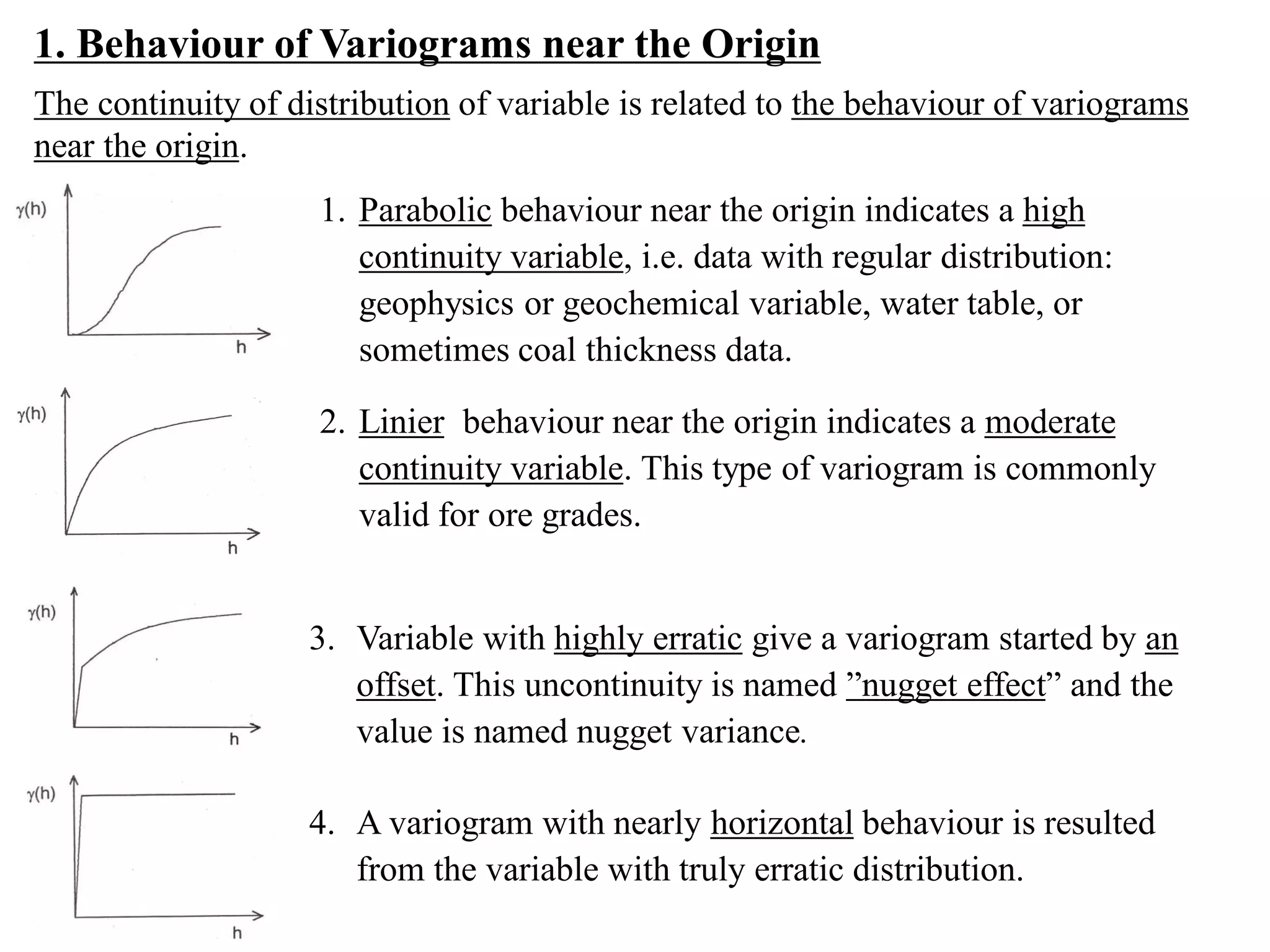
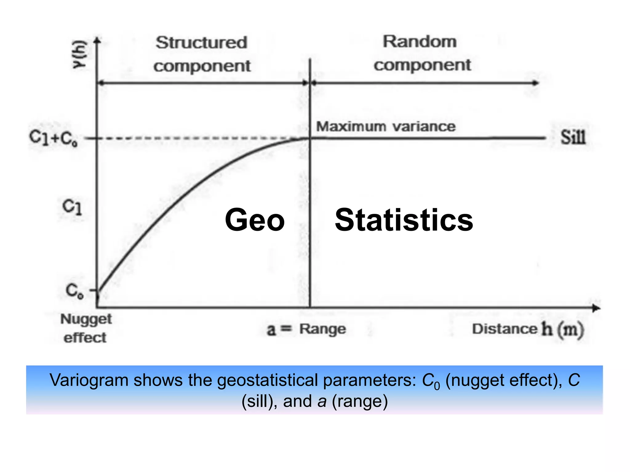
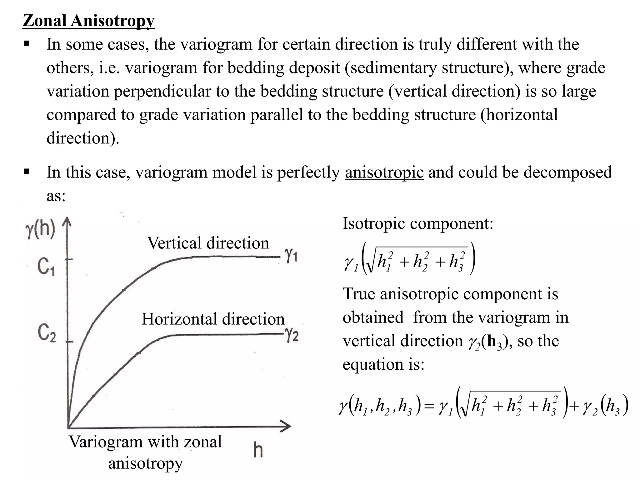
Material 5:
Spatial Structure of
Variogram
TA5212 Applied Geostatistics
1. Behaviour of Variograms near the Origin
1. Parabolic behaviour near the origin indicates a high
continuity variable, i.e. data with regular distribution:
geophysics or geochemical variable, water table, or
sometimes coal thickness data.
2. Linier behaviour near the origin indicates a moderate
continuity variable. This type of variogram is commonly
valid for ore grades.
3. Variable with highly erratic give a variogram started by an
offset. This uncontinuity is named ”nugget effect” and the
value is named nugget variance.
4. A variogram with nearly horizontal behaviour is resulted
from the variable with truly erratic distribution.
The continuity of distribution of variable is related to the behaviour of variograms
near the origin.
2. Area of Influence (Range)
▪ Commonly (h) will be increasing while h is
increasing, it means that the magnitude of the
difference of values between two points is
dependant on the distance of both.
▪ The increasing of (h) is still occurred as long as
the values among points are still influenced each
others, the area of them is named area of
influence. (h) will be constant up to a value of
() = C (sill) which actually is population
variance (variance a priori).
▪ The area of influence has notation a (range).
Beyond this distance, the average of variation of
values Z(x) and Z(x+h) are not dependant
anymore, or Z(x) and Z(x+h) are not correlated
each others. Range a is a measure of area of
influence.
Variogram shows the geostatistical parameters: C0 (nugget effect), C
(sill), and a (range)
Geo Statistics
3. Nested Structures
▪ If an ore deposit has some different
structures (scales), then each of them
will give variograms with different
range (a) (a measure on dimension of
structures). This influence of
structures will be overlaid, so they will
give a combined variogram which the
components can be decomposed.
▪ Variogram with nested structure is
commonly occured if the distance
between samples is very close
compared to the range a. These
variograms were ussually occurred on
fluviatil deposit with lens or fingering
shaped.
Local
structure
Regional
structure
4. Nugget Variance and Micro Structure
▪ Variogram with nested structure is
commonly occurred if the distance of
samples is very close compared to the
range a. In case the lag distance is
chosen largerly then the origin of
variogram could not be recorded well,
therefore the curve extrapolation toward
h = 0 will not give (0) = 0, but (0) =
C0 which is known as nugget variance.
▪ The influence of micro structure for
choosing the lag distance can be seen by
the presence or absence of nugget
variance. The nugget effect can be
minimized by reducing the lag distance h.
The presence of nugget variance also
could be caused by the sampling error,
error in grades analyzes, etc.
5. Anisotropy
Due to h is a vector, then a variogram must be defined for any distances. An
observation for the change of (h) according to their direction is possible to generate
an anisotropy.
Isotropy
If the variogram for any distances are the same, then (h) is a function of the
absolute value of vector where: , if h1, h2, and h3 are
components of vector h.
Geometrical Anisotropy
▪ If some (h) with different direction has the same sill C and nugget variance,
while the ranges a are different, then they shows geometrical anisotropy.
▪ In common the magnitude of range a will be distributed following an ellipsoid.
This phenomena could be occurred for placer deposit (tin, gold, iron sand, etc.).
h
 2
3
2
2
2
1 h
h
h
h +
+
=
aN-S : range for N – S direction
aNE-SW : range for NE – SW direction
aE-W : range for E – W direction
aNW-SE : range for NW – SE direction
A pattern of geometrical
anisotropy (ellipsoid)
aN-S aNE-SW aE-W aNW-SE
aN-S
aNE-SW
aE-W
aNW-SE
Variogram with
Geometrical
Anisotropy
Some anisotropy
phenomena in
lateritic nickel
deposit
Some anisotropy
phenomena in the
parameters of coal
quality and geometry:
(a) Ash content
(b) Calorific value
(c) Total sulphur
(d) Thickness
(a) (b)
(d)
(c)
3D Ellipsoid Anisotropy
Horizontal Isotropy +
Vertical Anisotropy
Zonal Anisotropy
▪ In some cases, the variogram for certain direction is truly different with the
others, i.e. variogram for bedding deposit (sedimentary structure), where grade
variation perpendicular to the bedding structure (vertical direction) is so large
compared to grade variation parallel to the bedding structure (horizontal
direction).
▪ In this case, variogram model is perfectly anisotropic and could be decomposed
as:
Isotropic component:
True anisotropic component is
obtained from the variogram in
vertical direction 2(h3), so the
equation is:
( )
2
3
2
2
2
1
1 h
h
h +
+

( ) ( ) ( )
3
2
2
3
2
2
2
1
1
3
2
1 h
h
h
h
h
,
h
,
h 

 +
+
+
=
Vertical direction
Horizontal direction
Variogram with zonal
anisotropy
6. Proportional Effect
In some cases, the variances in an area depends on the local mean. This could be
seen from the relationship between variance and the square of means, i.e. in drilling
group data set.
Example: Relationship between variance (2) and local mean (Z2) for Mo deposit,
and the variograms for each level with different values of ().
If the relationship between variance and square of local mean is linear, then their
relative variogram could be defined, i.e. each steps of experimental variogram
calculation must be divided by the square of local mean:
( )
( ) ( )
  ( )
( )
 2
h
N
1
i
2
h
i
i
)
h
(
Z
h
N
/
x
z
x
z
2
1
h

=
+
−
=

( ) ( ) ( )
 
 
( )
( )
h
N
/
2
/
x
Z
x
Z
2
1
h
Z
h
N
1
i
h
i
i

=
+
−
=
with
So the relative variogram could be obtained as below. The phenomena of
proportionaal effect can be found commonly for data with lognormal distribution.
The relative variogram
7. Drift
Drift is found for the variogram with normal behaviour in the beginning, i.e. it
rises up to the sill, but abruptly it rises up again as parabolic. It means that the
regionalized variables is not stationary anymore. The drift could be defined easily
by calculating the mean difference of variables xi and xi+h according to their
vector direction h:
( ) ( ) ( )
  ( )
( )

=
+ 





−
=
h
N
1
i
h
i
i h
N
/
x
Z
x
Z
2
1
2
1
h

and then visualized as graph. If the drift is absent, then the value of ∆(h) will be
scattered around the axis of h.
An example of parabolic
effect of a drift of the
variogram of: (A) sulphur of
coal mine, and (B) lead of Pb-
Zn mine.
8. Hole Effect
▪ When the variogram is calculated along the data distribution with high values
and then low values, i.e. grades of channel sampling across ore veins, then after
reaching the sill, it will be rising up and going down periodically.
▪ Below is an example of hole effect from Clark (Practical Geostatistics) and
Journel & Huijbregts (Mining Geostatistics).
An example of
variogram with
hole effect
Distance (meter)
Experimental
variogram
(%Zn)
2
Directional variograms of the gold accumulations; (a) parallel with
the direction of the current and (b) perpendicular to it (Armstrong,
1998)
1646367063278_Material-5---Spatial-Structure-of-Variogram.pdf

1646367063278_Material-5---Spatial-Structure-of-Variogram.pdf

  • 1.
    Material 5: Spatial Structureof Variogram TA5212 Applied Geostatistics
  • 2.
    1. Behaviour ofVariograms near the Origin 1. Parabolic behaviour near the origin indicates a high continuity variable, i.e. data with regular distribution: geophysics or geochemical variable, water table, or sometimes coal thickness data. 2. Linier behaviour near the origin indicates a moderate continuity variable. This type of variogram is commonly valid for ore grades. 3. Variable with highly erratic give a variogram started by an offset. This uncontinuity is named ”nugget effect” and the value is named nugget variance. 4. A variogram with nearly horizontal behaviour is resulted from the variable with truly erratic distribution. The continuity of distribution of variable is related to the behaviour of variograms near the origin.
  • 3.
    2. Area ofInfluence (Range) ▪ Commonly (h) will be increasing while h is increasing, it means that the magnitude of the difference of values between two points is dependant on the distance of both. ▪ The increasing of (h) is still occurred as long as the values among points are still influenced each others, the area of them is named area of influence. (h) will be constant up to a value of () = C (sill) which actually is population variance (variance a priori). ▪ The area of influence has notation a (range). Beyond this distance, the average of variation of values Z(x) and Z(x+h) are not dependant anymore, or Z(x) and Z(x+h) are not correlated each others. Range a is a measure of area of influence.
  • 4.
    Variogram shows thegeostatistical parameters: C0 (nugget effect), C (sill), and a (range) Geo Statistics
  • 5.
    3. Nested Structures ▪If an ore deposit has some different structures (scales), then each of them will give variograms with different range (a) (a measure on dimension of structures). This influence of structures will be overlaid, so they will give a combined variogram which the components can be decomposed. ▪ Variogram with nested structure is commonly occured if the distance between samples is very close compared to the range a. These variograms were ussually occurred on fluviatil deposit with lens or fingering shaped. Local structure Regional structure
  • 6.
    4. Nugget Varianceand Micro Structure ▪ Variogram with nested structure is commonly occurred if the distance of samples is very close compared to the range a. In case the lag distance is chosen largerly then the origin of variogram could not be recorded well, therefore the curve extrapolation toward h = 0 will not give (0) = 0, but (0) = C0 which is known as nugget variance. ▪ The influence of micro structure for choosing the lag distance can be seen by the presence or absence of nugget variance. The nugget effect can be minimized by reducing the lag distance h. The presence of nugget variance also could be caused by the sampling error, error in grades analyzes, etc.
  • 7.
    5. Anisotropy Due toh is a vector, then a variogram must be defined for any distances. An observation for the change of (h) according to their direction is possible to generate an anisotropy. Isotropy If the variogram for any distances are the same, then (h) is a function of the absolute value of vector where: , if h1, h2, and h3 are components of vector h. Geometrical Anisotropy ▪ If some (h) with different direction has the same sill C and nugget variance, while the ranges a are different, then they shows geometrical anisotropy. ▪ In common the magnitude of range a will be distributed following an ellipsoid. This phenomena could be occurred for placer deposit (tin, gold, iron sand, etc.). h  2 3 2 2 2 1 h h h h + + =
  • 8.
    aN-S : rangefor N – S direction aNE-SW : range for NE – SW direction aE-W : range for E – W direction aNW-SE : range for NW – SE direction A pattern of geometrical anisotropy (ellipsoid) aN-S aNE-SW aE-W aNW-SE aN-S aNE-SW aE-W aNW-SE Variogram with Geometrical Anisotropy
  • 9.
  • 10.
    Some anisotropy phenomena inthe parameters of coal quality and geometry: (a) Ash content (b) Calorific value (c) Total sulphur (d) Thickness (a) (b) (d) (c)
  • 11.
    3D Ellipsoid Anisotropy HorizontalIsotropy + Vertical Anisotropy
  • 12.
    Zonal Anisotropy ▪ Insome cases, the variogram for certain direction is truly different with the others, i.e. variogram for bedding deposit (sedimentary structure), where grade variation perpendicular to the bedding structure (vertical direction) is so large compared to grade variation parallel to the bedding structure (horizontal direction). ▪ In this case, variogram model is perfectly anisotropic and could be decomposed as: Isotropic component: True anisotropic component is obtained from the variogram in vertical direction 2(h3), so the equation is: ( ) 2 3 2 2 2 1 1 h h h + +  ( ) ( ) ( ) 3 2 2 3 2 2 2 1 1 3 2 1 h h h h h , h , h    + + + = Vertical direction Horizontal direction Variogram with zonal anisotropy
  • 13.
    6. Proportional Effect Insome cases, the variances in an area depends on the local mean. This could be seen from the relationship between variance and the square of means, i.e. in drilling group data set. Example: Relationship between variance (2) and local mean (Z2) for Mo deposit, and the variograms for each level with different values of ().
  • 14.
    If the relationshipbetween variance and square of local mean is linear, then their relative variogram could be defined, i.e. each steps of experimental variogram calculation must be divided by the square of local mean: ( ) ( ) ( )   ( ) ( )  2 h N 1 i 2 h i i ) h ( Z h N / x z x z 2 1 h  = + − =  ( ) ( ) ( )     ( ) ( ) h N / 2 / x Z x Z 2 1 h Z h N 1 i h i i  = + − = with So the relative variogram could be obtained as below. The phenomena of proportionaal effect can be found commonly for data with lognormal distribution. The relative variogram
  • 15.
    7. Drift Drift isfound for the variogram with normal behaviour in the beginning, i.e. it rises up to the sill, but abruptly it rises up again as parabolic. It means that the regionalized variables is not stationary anymore. The drift could be defined easily by calculating the mean difference of variables xi and xi+h according to their vector direction h: ( ) ( ) ( )   ( ) ( )  = +       − = h N 1 i h i i h N / x Z x Z 2 1 2 1 h  and then visualized as graph. If the drift is absent, then the value of ∆(h) will be scattered around the axis of h. An example of parabolic effect of a drift of the variogram of: (A) sulphur of coal mine, and (B) lead of Pb- Zn mine.
  • 16.
    8. Hole Effect ▪When the variogram is calculated along the data distribution with high values and then low values, i.e. grades of channel sampling across ore veins, then after reaching the sill, it will be rising up and going down periodically. ▪ Below is an example of hole effect from Clark (Practical Geostatistics) and Journel & Huijbregts (Mining Geostatistics). An example of variogram with hole effect Distance (meter) Experimental variogram (%Zn) 2
  • 17.
    Directional variograms ofthe gold accumulations; (a) parallel with the direction of the current and (b) perpendicular to it (Armstrong, 1998)