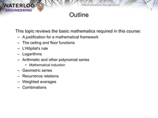
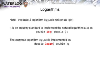
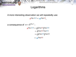
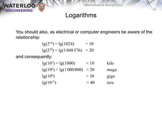
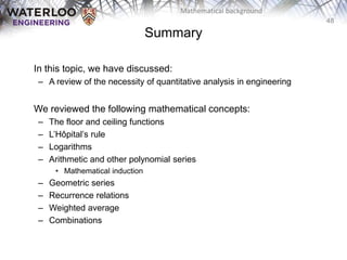
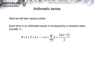
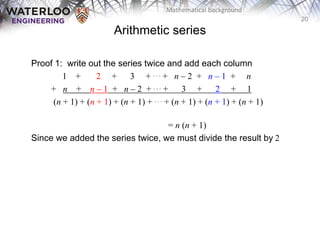
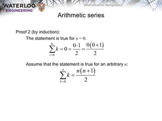
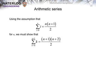
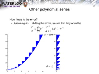
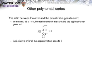
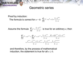
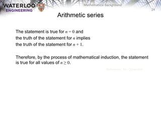
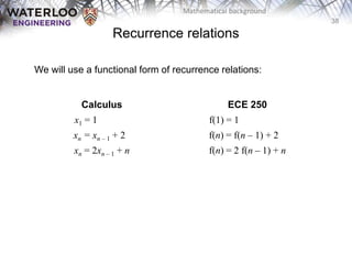
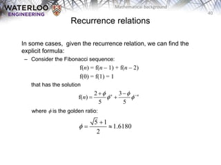
This document provides an overview of various mathematical topics required for an algorithms and data structures course, including: - Justification for using quantitative methods like mathematics to evaluate algorithms and data structures. - Common functions like floor, ceiling, and logarithms. - Properties and proofs of arithmetic series, geometric series, and other polynomial series. - Introduction of concepts like mathematical induction that will be used throughout the course.

1. ECE 250 Algorithms and Data Structures
Douglas Wilhelm Harder, M.Math. LEL
Department of Electrical and Computer Engineering
University of Waterloo
Waterloo, Ontario, Canada
ece.uwaterloo.ca
dwharder@gmail.com
© 2006-2018 by Douglas Wilhelm Harder. Some rights reserved.
Mathematical background

2. 2
Mathematical background
This topic reviews the basic mathematics required in this course:
– A justification for a mathematical framework
– The ceiling and floor functions
– L’Hôpital’s rule
– Logarithms
– Arithmetic and other polynomial series
• Mathematical induction
– Geometric series
– Recurrence relations
– Weighted averages
– Combinations
Outline

3. 3
Mathematical background
Mathematics and engineering
For engineers, mathematics is a tool:
– Of course, that doesn’t mean it always works...
http://xkcd.com/55/

4. 4
Mathematical background
Justification
However, as engineers, you will not be paid to say:
Method A is better than Method B
or
Algorithm A is faster than Algorithm B
Such comparisons are said to be qualitative:
qualitative, a. Relating to, connected or concerned with, quality or qualities.
Now usually in implied or expressed opposition to quantitative.
OED

5. 5
Mathematical background
Qualitative statements cannot guide engineering design decisions:
– Algorithm A could be better than Algorithm B, but Algorithm A would
require three person weeks to implement, test, and integrate while
Algorithm B has already been implemented and has been used for the
past year
– There are circumstances where it may beneficial to use Algorithm A, but
not based on the word better
Justification

6. 6
Mathematical background
Thus, we will look at a quantitative means of describing data
structures and algorithms:
quantitative, a. Relating to, concerned with, quantity or its measurement;
ascertaining or expressing quantity. OED
This will be based on mathematics, and therefore we will look at a
number of properties which will be used again and again throughout
this course
Justification

7. 7
Mathematical background
Floor and ceiling functions
The floor function maps any real number x onto the greatest integer
less than or equal to x:
– Consider it rounding towards negative infinity
The ceiling function maps x onto the least integer greater than or
equal to x:
– Consider it rounding towards positive infinity
– The cmath library implements these as
double floor( double ); double ceil( double );
3.2 3 3
5.2 6 6
 
   
   
    
   
   
3.2 4 4
5.2 5 5
 
   
   
    
   
   
Necessary because double
have a range just under 21024
long can only represent
numbers as large as 263 – 1

8. 8
Mathematical background
L’Hôpital’s rule
If you are attempting to determine
but both , it follows
Repeat as necessary…
 
 
lim
n
f n
g n

   
lim lim
n n
f n g n
 
  
 
 
 
 
 
 
1
1
lim lim
n n
f n f n
g n g n
 

 
 
k
f n
Note: the kth derivative will always be shown as

9. 9
Mathematical background
We will begin with a review of logarithms:
If n = em, we define
m = ln( n )
It is always true that eln(n) = n; however, ln(en) = n requires that n is
real
Logarithms

10. 10
Mathematical background
Exponentials grow faster than any non-constant polynomial
for any d > 0
Thus, their inverses—logarithms—grow slower than any polynomial
Logarithms
lim
n
d
n
e
n

 
ln( )
lim 0
d
n
n
n



11. 11
Mathematical background
Example: is strictly greater than ln(n)
1/2
( )
f n n n
 
ln(n)
n
Logarithms

12. 12
Mathematical background
Logarithms
grows slower but only up to n = 93
(93.354, 4.536)
ln(n)
3
n
1/3 3
( )
f n n n
 

13. 13
Mathematical background
You can view this with any polynomial
ln(n)
4
n
Logarithms
(5503.66, 8.61)

14. 14
Mathematical background
We have compared logarithms and polynomials
– How about log2(n) versus ln(n) versus log10(n)
You have seen the formula
All logarithms are scalar multiples of each others
)
ln(
)
ln(
)
(
log
b
n
n
b 
Logarithms
Constant

15. 15
Mathematical background
A plot of log2(n) = lg(n), ln(n), and log10(n)
lg(n)
ln(n)
log10(n)
Logarithms

16. 16
Mathematical background
Note: the base-2 logarithm log2(n) is written as lg(n)
It is an industry standard to implement the natural logarithm ln(n) as
double log( double );
The common logarithm log10(n) is implemented as
double log10( double );
Logarithms

17. 17
Mathematical background
A more interesting observation we will repeatedly use:
nlogb (m) = mlogb(n),
a consequence of :
nlogb (m) = (blogb(n))logb(m)
= blogb(n) logb(m)
= (blogb(m))logb(n)
= mlogb(n)
Logarithms
logb n
n b


18. 18
Mathematical background
You should also, as electrical or computer engineers be aware of the
relationship:
lg(210) = lg(1024) = 10
lg(220) = lg(1048576) = 20
and consequently:
lg(103) = lg(1000) ≈ 10 kilo
lg(106) = lg(1000000) ≈ 20 mega
lg(109) ≈ 30 giga
lg(1012) ≈ 40 tera
Logarithms

19. 19
Mathematical background
Next we will look various series
Each term in an arithmetic series is increased by a constant value
(usually 1) :
 
0
1
0 1 2 3
2
n
k
n n
n k


      

Arithmetic series

20. 20
Mathematical background
Proof 1: write out the series twice and add each column
1 + 2 + 3 + . . . + n – 2 + n – 1 + n
+ n + n – 1 + n – 2 + . . . + 3 + 2 + 1
(n + 1) + (n + 1) + (n + 1) + . . . + (n + 1) + (n + 1) + (n + 1)
= n (n + 1)
Since we added the series twice, we must divide the result by 2
Arithmetic series

21. 21
Mathematical background
Proof 2 (by induction):
The statement is true for n = 0:
Assume that the statement is true for an arbitrary n:
 
0
0
0 0 1
0 1
0
2 2
i
k



  

 
0
1
2
n
k
n n
k




Arithmetic series

22. 22
Mathematical background
Using the assumption that
for n, we must show that
 
0
1
2
n
i
n n
i




  
1
0
1 2
2
n
k
n n
k


 


Arithmetic series

23. 23
Mathematical background
Then, for n + 1, we have:
By assumption, the second sum is known:
 
1
0 0
1
n n
k i
k n k

 
  
 
 
 
   
  
1
1
2
1 2 1
2
1 2
2
n n
n
n n n
n n

  
  

 

Arithmetic series

24. 24
Mathematical background
The statement is true for n = 0 and
the truth of the statement for n implies
the truth of the statement for n + 1.
Therefore, by the process of mathematical induction, the statement
is true for all values of n ≥ 0.
Reference: Mr. Oprendick
Arithmetic series

25. 25
Mathematical background
We could repeat this process, after all:
however, it is easier to see the pattern:
 
2
2
3
0
1
4
n
k
n n
k




   3
2
0
1 2 1
6 3
n
k
n n n n
k

 
 

  
2
0
1 2 1
6
n
k
n n n
k

 


 
2
2 4
3
0
1
4 4
n
k
n n n
k


 

Other polynomial series
  2
0
1
2 2
n
k
n n n
k


 


26. 26
Mathematical background
We can generalize this formula
Demonstrating with d = 3 and d = 4:
1
0 1
d
n
d
k
n
k
d





Other polynomial series

27. 27
Mathematical background
The justification for the approximation is that we are approximating
the sum with an integral:
However, there is an
accumulating error:
1 1
0 0 0
0
1 1
n
n d d
n
d d
k x
x n
k x dx
d d
 
 
   
 
 
Other polynomial series
n2

28. 28
Mathematical background
How large is the error?
– Assuming d > 1, shifting the errors, we see that they would be
Other polynomial series
1
1
0
2 1
d d
n
d d d
k
n n
k n n
d



  


n2 = 100
n2 = 10

29. 29
Mathematical background
The ratio between the error and the actual value goes to zero:
– In the limit, as n → ∞, the ratio between the sum and the approximation
goes to 1
– The relative error of the approximation goes to 0
Other polynomial series
1
0
1
lim 1
d
n
n
d
k
n
d
k



 


30. 30
Mathematical background
The next series we will look at is the geometric series with common
ratio r:
and if |r| < 1 then it is also true that
1
0
1
1
n
n
k
k
r
r
r






0
1
1
k
k
r
r





Geometric series

31. 31
Mathematical background
Elegant proof: multiply by
Ref: Bret D. Whissel, A Derivation of Amortization
  0
0
0 0
2 2 1
1
1
1
1
(1 ) ( )
1
1
1
n k
n
k k
k
n n
k k
k k
n n n
n
r r
r
r
r r r
r
r r r r r r r
r
r
r


 








        







 
Geometric series
1
1
1
r
r



Telescoping series:
all but the first and last terms cancel

32. 32
Mathematical background
Proof by induction:
The formula is correct for n = 0:
Assume the formula is true for an arbitrary n; then
and therefore, by the process of mathematical
induction, the statement is true for all n ≥ 0.
0 1
0
0
0
1
1
1
k
k
r
r r
r



  


1
0
1
1
n
n
i
i
r
r
r






1 1 1
1
1 1
0 0
1 2 1 2 ( 1) 1
1 (1 ) 1
1 1
1 1 1
1 1 1
n n n
n n
k n k n
k k
n n n n n
r r r r
r r r r
r r
r r r r r
r r r
  

 
 
     
   
    
 
    
  
  
 
Geometric series

33. 33
Mathematical background
Note that we can use a change-of-index with summations like we do
with integration:
Letting j = i – 1:


 






n
i
i
n
i
i
n
i
i
r
r
rr
r
1
1
1
1
1
r
r
r
r
r
n
n
j
j



 


1
1
1
0
Geometric series

34. 34
Mathematical background
A common geometric series will involve the ratios r = ½ and r = 2:
  n
n
n
i
i














 2
2
1
1
2
1
2
1
1
2
1
0
1
1
0
1 2
2 2 1
1 2
n
n
k n
k




  


2
2
1
0










i
i
Geometric series

35. 35
Mathematical background
Finally, we will review recurrence relations:
– Sequences may be defined explicitly: xn = 1/n
1, 1/2, 1/3, 1/4, ...
– A recurrence relationship is a means of defining a sequence based on
previous values in the sequence
– Such definitions of sequences are said to be recursive
Recurrence relations

36. 36
Mathematical background
Define an initial value: e.g., x1 = 1
Defining xn in terms of previous values:
– For example,
xn = xn – 1 + 2
xn = 2xn – 1 + n
xn = xn – 1 + xn – 2
Recurrence relations

37. 37
Mathematical background
Given the two recurrence relations
xn = xn – 1 + 2 xn = 2xn – 1 + n
and the initial condition x1 = 1 we would like to find explicit formulae
for the sequences
In this case, we have
xn = 2n – 1 xn = 2n + 1 – n – 2
respectively
Recurrence relations

38. 38
Mathematical background
We will use a functional form of recurrence relations:
Calculus ECE 250
x1 = 1............. f(1) = 1...................
xn = xn – 1 + 2.. f(n) = f(n – 1) + 2...
xn = 2xn – 1 + n f(n) = 2 f(n – 1) + n
Recurrence relations

39. 39
Mathematical background
The previous examples using the functional notation are:
f(n) = f(n – 1) + 2 g(n) = 2 g(n – 1) + n
With the initial conditions f(1) = g(1) = 1, the solutions are:
f(n) = 2n – 1 g(n) = 2n + 1 – n – 2
Recurrence relations

40. 40
Mathematical background
In some cases, given the recurrence relation, we can find the
explicit formula:
– Consider the Fibonacci sequence:
f(n) = f(n – 1) + f(n – 2)
f(0) = f(1) = 1
that has the solution
where f is the golden ratio:
2 3
f( )
5 5
n n
n
f f
f f
 
 
5 1
1.6180
2
f

 
Recurrence relations

41. 41
Mathematical background
Weighted averages
Given n objects x1, x2, x3, ..., xn, the average is
Given a sequence of coefficients c1 , c2 , c3 , … , cn where
then we refer to
as a weighted average
For an average,
1 2 3 n
x x x x
n
   
1 2 3 1
n
c c c c
    
1 1 2 2 3 3 n n
c x c x c x c x
   
1 2 3
1
n
c c c c
n
    

42. 42
Mathematical background
Weighted averages
Examples:
– Simpson’s method approximates an integral by sampling
the function at three points: f(a), f(b), f(c)
– The average value of the function is approximated by
– It can be shown that that
is a significant better approximation than
     
1 2 1
6 3 6
f a f b f c
 
     
  
1 2 1
6 3 6
f a f b f c c a
  
     
 
3
f a f b f c
c a
 


43. 43
Mathematical background
Weighted averages
Examples:
– Using the weighted average:
– Using a simple average:
     
 
1 2 1
6 3 6
cos 0 cos 1 cos 2 2 0.9150
   
2
0
cos( ) sin(2) 0.9093
x dx  

     
cos 0 cos 1 cos 2
2 0.7494
3
 
 
1 2 1
6 3 6 1
  
1 1 1
3 3 3 1
  

44. 44
Mathematical background
Combinations
Given n distinct items, in how many ways can you choose k of these?
– I.e., “In how many ways can you combine k items from n?”
– For example, given the set {1, 2, 3, 4, 5}, I can choose three of these
in any of the following ways:
{1, 2, 3}, {1, 2, 4}, {1, 2, 5}, {1, 3, 4}, {1, 3, 5},
{1, 4, 5}, {2, 3, 4}, {2, 3, 5}, {2, 4, 5}, {3, 4, 5},
The number of ways such items can be chosen is written
where is read as “n choose k”s
There is a recursive definition:
 
!
! !
n n
k k n k
 

 

 
n
k
 
 
 
1 1
1
n n n
k k k
 
     
 
     

     

45. 45
Mathematical background
Combinations
The most common question we will ask in this vein:
– Given n items, in how many ways can we choose two of them?
– In this case, the formula simplifies to:
For example, given {0, 1, 2, 3, 4, 5, 6}, we have the following 21 pairs:
{0, 1}, {0, 2}, {0, 3}, {0, 4}, {0, 5}, {0, 6},
{1, 2}, {1, 3}, {1, 4}, {1, 5}, {1, 6},
{2, 3}, {2, 4}, {2, 5}, {2, 6},
{3, 4}, {3, 5}, {3, 6},
{4, 5}, {4, 6},
{5, 6}
 
 
1
!
2 2! 2 ! 2
n n n
n
n

 
 
 

 

46. 46
Mathematical background
Combinations
You have also seen this in expanding polynomials:
For example,
 
0
n
n k n k
k
n
x y x y
k


 
   
 

 
4
4 4
0
4 3 2 2 3 4
4 3 2 2 3 4
4
4 4 4 4 4
0 1 2 3 4
4 6 4
k k
k
x y x y
k
y xy x y x y x
y xy x y x y x


 
   
 
         
    
         
         
    


47. 47
Mathematical background
Combinations
These are also the coefficients of Pascal’s triangle:
0
0
1 1
0 1
2 2 2
0 1 2
3 3 3 3
0 1 2 3
4 4 4 4 4
0 1 2 3 4
 
 
 
   
   
   
     
     
     
       
       
       
         
         
         
1
1 1
1 2 1
1 3 3 1
1 4 6 4 1

48. 48
Mathematical background
In this topic, we have discussed:
– A review of the necessity of quantitative analysis in engineering
We reviewed the following mathematical concepts:
– The floor and ceiling functions
– L’Hôpital’s rule
– Logarithms
– Arithmetic and other polynomial series
• Mathematical induction
– Geometric series
– Recurrence relations
– Weighted average
– Combinations
Summary

49. 49
Mathematical background
[1] Cormen, Leiserson, and Rivest, Introduction to Algorithms,
McGraw Hill, 1990, Chs 2-3, p.42-76.
[2] Weiss, Data Structures and Algorithm Analysis in C++, 3rd Ed.,
Addison Wesley, §§ 1.2-3, p.2-11.
Reference

50. 50
Mathematical background
Usage Notes
• These slides are made publicly available on the web for anyone to
use
• If you choose to use them, or a part thereof, for a course at another
institution, I ask only three things:
– that you inform me that you are using the slides,
– that you acknowledge my work, and
– that you alert me of any mistakes which I made or changes which you
make, and allow me the option of incorporating such changes (with an
acknowledgment) in my set of slides
Sincerely,
Douglas Wilhelm Harder, MMath
dwharder@alumni.uwaterloo.ca