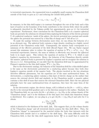
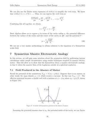
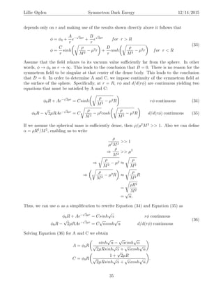
This document explores symmetron dark energy through an electrostatic analogy. It begins with background on the discovery of dark energy and models proposed to explain it, including the chameleon and symmetron scalar fields. It then discusses how electrostatic solutions can provide insights into these scalar fields under certain conditions. The document focuses on developing the massive electrostatic analogy for the symmetron field and examining its behavior outside a spherical object.
![Lillie Ogden Symmetron Dark Energy 12/14/2015
electrostatics in order to identofy that the Chameleon scalar field obeys an electrostatic analogy,
allowing us to find solutions to this complex field under certain, simplifying conditions. Next,
will will demonstrate how working with ellipsoidal objects as opposed to spherical objects may
increase experimental sensitivity due to the “lightning rod effect”. We then will introduce a
theoretical branch of electrostatics called massive electrostatics to show that, similarly, the
Symmetron obeys a massive electrostatic analogy and explore the behavior of the field outside
of a spherical object. Finally, we calculate Symmetron forces to explore the field’s affect in a
terrestrial environment.
2 History and Discovery of Dark Energy
Einstein’s theory of general relativity yielded a concise, mathematical tool for describing the
arrangement of matter in space and was immediately recognized by the scientific community
as having profound ramifications for the field of physics and cosmology. These implications
were encapsulated in a packet of field equations and these set foundation for future research in
the field of cosmology. Similar to how Maxwell’s Equations describe the electromagnetic fields
by evaluating the presence of charges and currents, the Einstein Field equations describe the
spacetime geometry resulting from the presence of mass and energy:
Gµν = 8πGTµν. (1)
These equations determine a metric tensor of spacetime for a given configuration of energy
and stress in the universe. The left hand side of the equation, Gµν, describes the geometry
and structure of the universe. The right hand side of Equation (1), 8πGTµν, describes the
composition of the universe including mass, energy, stress, and density. The equations indicate
that the composition of the universe determines how spacetime curves and in turn, curved
spacetime determines the behavior of the composition.
Further, the equations implied that the universe was dynamic because they consisted of
differential equations, changing in time and space. However, the common worldview at the
time believed that the universe was fixed and unchanging [1]. Thus, Einstein first attempted to
a fabricate a solution with a static universe. What he found was that if the universe were static
at the beginning of time, the gravitational attraction in his equations would have resulted in
the collapse of the universe, suggesting that the universe was indeed dynamic. However, given
the apparent stationary and stable nature of the universe, Einstein proposed that there must
be some device that he had missed working to hinder and cancel out the gravitational force and
create the static universe. He stabilized his theory to account for this anti-gravity by adding
a simple, non-zero cosmological constant in his equation. The “cosmological constant” term
represented only a hypothetical entity that could counteract gravity and therefore stabilize the
universe against gravitational collapse. In fact in a paper written by Einstein in 1917, he stated
“The term is necessary only for the purpose of making possible a quasi-static distribution of
matter, as required by the fact of the small velocities of the star.”[2]
6](https://image.slidesharecdn.com/e63894b1-155e-45af-a04b-329fba2c97ba-160321203613/85/Dark-Energy-Thesis-6-320.jpg)
![Lillie Ogden Symmetron Dark Energy 12/14/2015
2.1 Hubble’s Discovery
The overarching belief that the universe was static was invalidated by tangible data and ob-
servations. In 1929, Hubble was studying light coming from galaxies at various distances from
earth and was able to determine that the further from earth the galaxy was located, the greater
the receding velocity of a galaxy. Hubble’s observations that light showed a red shift that in-
creased with distance ruled out the possibility of the Einstein static state model. In fact, with
the data, Hubble conjectured that the universe was not only dynamic but was expanding. This
“cosmic expansion”, as it became known as, meant that the light from distant galaxies was red-
shifted because the galaxies were in fact moving away from us and from all the other galaxies
in the universe. Space itself was expanding between the matter in the universe. Therefore,
the farther any two galaxies were from each other, the faster they continued to move apart
and separate. Hubble published this linear proportionality between distance and velocity and
the Hubble Constant is now the unit of measurement that is used to describe the expansion of
the universe. Cosmologists quickly recognized that an expanding universe meant that in the
future, the galaxies would lie farther apart. However, they also extrapolated that in the past,
the galaxies must have been much closer together and the universe must have been far more
dense. In fact, at some point in time, the universe would have been contained in the size of the
atom. Thus this data led to the theory of the Big Bang, which was essentially confirmed with
the discovery of the CMB in the late 20th century.
2.2 The Friedmann-Walker-Robertson Metric
After Hubble’s eminent discovery, Einstein’s field equations had to be solved for new models
that allowed for a dynamic and complex universe. In the 1920’s, mathematician Alexander
Friedmann was credited with designing a set of possible mathematical solutions that gave a non-
static universe [1]. Einstein’s original static state solution used the simplifying assumption that
the universe was spatially homogeneous and isotropic, meaning that it appeared the same no
matter where in the universe a person stood and what direction they looked. This homogeneity
and isotropy of the universe became known as the Cosmological Principle. Friedmann’s metric
maintained a universe that was homogeneous and isotropic, but that was no longer static. This
metric, called the Friedmann-Walker-Robertson, metric is given as
−c2
dT2
= −c2
dt2
+ a2
(t)
dr2
1 − kr2
+ r2
dθ2
+ r2
sin2
θdφ2
, (2)
where k is an important parameter that describes the curvature of spacetime. In the 1930s,
Robertson and Walker showed that there were only three possible spacetime metrics for a
universe that were consistent with the Cosmological Principle: k = ±1, 0 [3]. If k = 1, then
the universe is said to be positively curved or closed. If k = −1, then the universe is said to be
negatively curved or open. If k = 0 then the universe is said to be “flat”. If the geometry is flat
then, the universe will stop expanding after infinite time and spacetime geometry is euclidean
on cosmic scales. Scientists began to explore these three cases in order to gain intuition about
the structure of the universe. Considering the case where the universe is flat (k = 0), one can
solve for the density of the universe that enables it to be flat. This is called the critical density
7](https://image.slidesharecdn.com/e63894b1-155e-45af-a04b-329fba2c97ba-160321203613/85/Dark-Energy-Thesis-7-320.jpg)
![Lillie Ogden Symmetron Dark Energy 12/14/2015
and is given by
ρcrit =
3H2
8πG
(3)
where H = ˙a/a is the Hubble constant and describes the evolution of the metric in terms of
expansion. In the constant, a is called the scale factor and multiplies the spatial components in
the FRW metric and ˙a is the time derivative of a. Cosmologists frequently describe the energy
density of the universe in terms of the density parameter Ω. It is defined as the ratio of the
density of some configuration of spacetime relative to the critical density:
Ω =
ρ
ρcrit
(4)
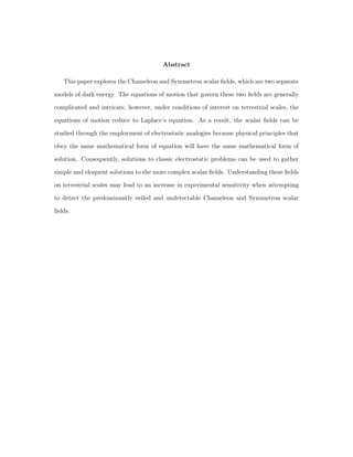
We can now define flat, open and closed in terms of the density parameter and portray the
scenarios graphically in Figure (1). A flat universe is when k = 0, ρ = ρcrit and Ω = 1.
This means that the universe is flat on a large scale and contains the critical density. An
open universe has values k = −1 , ρ < ρcrit and Ω < 1. This means that the universe is
negatively curved and the density of the universe, related to the amount of mass and energy
in the universe, is less than the critical density required to have a flat universe. Thus, in an
open universe, there is insufficient energy density to counteract or reverse the expansion due
to gravity and the universe expands forever as galaxies fly apart from each other, named the
“Big Freeze” because the universe will slowly cool as it expands. A closed universe is when
k = 1, ρ > ρcrit and Ω > 1. This means that the universe is positively curved and excess energy
density in the universe counteracts the tendency of the universe to expand, causing the universe
to eventually collapse back on itself due to gravitational attraction, called the “Big Crunch”.
Figure 1: The fate of a universe as it evolves according to Einstein’s field equations under situations with different amounts of
density, form NASA and WMAP. If the density of the universe is less than the critical density, then the universe will expand forever,
like the red curve in the graph above. This is also known as the“Big Freeze”. If the density of the universe is greater than the
critical density, then gravity will eventually win and the universe will collapse back on itself, the so called “Big Crunch”, like the
graph’s orange curve. [4]
8](https://image.slidesharecdn.com/e63894b1-155e-45af-a04b-329fba2c97ba-160321203613/85/Dark-Energy-Thesis-8-320.jpg)
![Lillie Ogden Symmetron Dark Energy 12/14/2015
Cosmologists contend that this theoretical line of thinking points to a universe that must
be flat. First, the fact that the universe is thirteen billion years old and it looks the way it does
today, with stars and galaxies populating the night sky, points to a flat universe. Consider a
universe that started with an initial density slightly less than the critical density, Ω = .999999
ie. an open universe. Then, the universe would have evolved according to the Einstein field
equations and by the time it was 13.7 billion years old, it would not have formed structures
that are bound by gravity. In other words, it would have expanded indefinitely and would
appear nothing like the universe we encounter today. On the other hand, consider a universe
that started with an initial density slightly larger than the critical density, Ω = 1.0000001 ie.
a closed universe. Then, the universe would have already collapsed after 13.7 billion years.
Therefore, the only way to have a universe that is stable and occupied by structures, galaxies,
and stars is if it started flat and has always been flat. The Friedmann-Walker-Robertson metric,
a solution to the Einstein field equations, enabled a theoretical line of thinking that demanded
a stable universe to be flat. Today, Friedmann is applauded for his ingenuity but during the
1920s, neither Einstein nor anyone else took any interest in Friedmann’s work, which they saw as
merely an abstract theoretical curiosity [1]. However, the metric has proofed a crucial solution
that permits concrete models of the mathematical composition of matter in the universe.
2.3 Discovery of the Cosmic Microwave Background
In the 1960s, new technologies enabled the discovery of the cosmic microwave background
(CMB), which helped to promote the notion of a flat universe and finally wipe out steady
state models. The detection of the CMB radiation was the most impressive piece of evidence
confirming the Big Bang theory. The CMB is the ancient, constant light source that permeates
through and saturates the universe. The start of our universe was a Big Bang 13.7 billion
years ago; a small, hot, dense event that sent the universe into a rapid inflationary epoch. This
inflationary epoch was immense enough to flatten the geometry of the universe. After the initial
burst of expansion, the rapid inflation disappeared and the universe resumed a more constant
expansion rate. This allowed the universe to cool and particles to form atoms. This cooling
left an imprint that permeated through space-a constant background radiation that glows at
a temperature just above absolute zero, about 2.7 K, and is uniformly distributed. However,
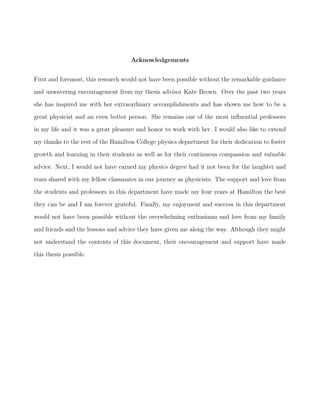
strictly speaking the CMB it is not entirely uniform and improved technologies and instruments
have detected tiny variations in the early temperature of the universe, which are produced by
variations in the early distribution of matter, shown in Figure (2).
With CMB data of the early temperature fluctuations, scientists can detect slightly denser
spots in the early universe where galaxies were eventually born out of and these regions were
extremely sensitive to the initial conditions of the geometry of the universe. The tempera-
ture fluctuations are consistent with an initial geometry corresponding to a primitive universe
that was flat. With the discovery of the CMB, and previous theoretical reasoning from the
FRW solution to Einstein’s equations, the flat universe became the dominant paradigm within
cosmology.
9](https://image.slidesharecdn.com/e63894b1-155e-45af-a04b-329fba2c97ba-160321203613/85/Dark-Energy-Thesis-9-320.jpg)
![Lillie Ogden Symmetron Dark Energy 12/14/2015
Figure 2: Temperature fluctuations of the CMB in the early universe, taken by the WMAP. [5]
A thorough comprehension was beginning to come together regarding the arrangement and
structure of the universe as data from new technology and cosmologists continued to confirm the
flat, dynamic nature of the universe. However, one large gap in the understanding of the cosmos
was entirely perplexing. Since the universe appeared flat, the contents in the universe must
sum to the critical density, Ω = 1, according the the FWR metric. However, measurements of
illuminating energy density in the form of baryonic matter such as stars, planets, galaxies, etc.
only make up 4.6% of the energy density required for a flat universe. Scientists were bewildered
by the apparent lack of energy density in the universe. Either the universe must not be flat and
cosmologists had the daunting, nearly impossible task of explaining the temperature fluctuations
in the CMB or the current technology could not detect the missing energy density in the
universe. Many scientists favor the latter option because current technology only enables us to
explore the luminous matter. The CMB made observations in the 1960’s of dark matter, which
scientist believe composes 23% of the density. Dark matter is believed to resemble ordinary
matter, differing only in that it has a reduced frequency of interacting with its surroundings.
That leaves about 72% of critical density unaccounted for. This 72% of the composition of the
universe is what scientists call dark energy. Many people were skeptical of the theory of dark
energy and worked at finding alternative explanations of the apparent lack of density.
2.4 Type 1a Supernovae
In the late 1990’s, Saul Perlmutter, Riess, and Schmidt were able to counteract the skepticism
regarding dark energy with his research on light emission from supernovae [6]. A supernovae
is the event of a dying white dwarf that explodes after it has reached a critical density and
thus, releases a large amount of radiation. In particular, he was examining type 1a super-
novae, which are especially unique because they emit the same amount of radiation for every
explosion. Therefore, the brightness observed on earth from a supernovae is proportional to
the distance that the star is away from earth since radiation goes as 1/r2
. Perlmutter and
others found that all the nearby supernovae had the predicted luminosity based on our un-
derstanding of nuclear processes, but the supernovae in a certain far range were dimmer than
10](https://image.slidesharecdn.com/e63894b1-155e-45af-a04b-329fba2c97ba-160321203613/85/Dark-Energy-Thesis-10-320.jpg)
![Lillie Ogden Symmetron Dark Energy 12/14/2015
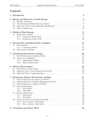
the science could explain. At the time of this discovery, many scientists suspected that the
universe was slowing in its expansion due to the force of gravity. However, the results from
the supernovae data, presented in Figure (3), showed that distant type 1a supernovas were
dimmer than expected, which was interpreted as the accelerated expansion of the universe.
This is called “cosmic acceleration” and was yet another marvel in cosmology. Some force
was dominating the expansion of the universe only in a certain redshift distance range of the
universe causing increased expansion that could not be explained with only matter and dark
matter. However, when dark energy was included into the equation, the data made sense.
Thus, type 1a supernovae data provided enormous support for the theory of dark energy, and
Perlmutter, Riess, and Schmidt were awarded the Nobel Prize in 2011 for their discovery [6].
Figure 3: A plot of the distance and luminos-
ity of type 1a supernovae. For far distances, the
luminosity is dimmer than predicted. [7]
Dark energy has become a model that not only would
account for the extra density needed for a flat universe,
but also provide the force that works to counteract grav-
ity in the Einstein Field Equations and cause the cosmic
expansion observed by Perlmutter, Riess, and Schmidt.
There have been several other credible arguments and ob-
servations that support the theory of dark energy. Con-
sequently, the current acceptance of the composition of
the universe is one in which baryonic matter constitutes
roughly 5%, dark matter constitutes roughly 25%, and
dark energy constitutes the remaining 70% of the energy
density [3]. Thus, the fundamental interpretation of the
cosmos once again changed and cosmologists were forced
to delve into the world of dark energy, an important field
in modern cosmology. Such a force would explain new
realms of cosmology and fill in the gaps in the field as a
whole, but it currently lacks a compelling model and sev-
eral scientists still doubt its existence. If dark energy does
exist, it has three defining characteristics. First, it does
not interact electromagnetically, thus why it is called dark.
Second, it must possess energy, as it is a form of energy
density. And lastly, it has the opposite effect of gravity
and can dominate in distant regions of space, causing cosmic acceleration. Apart from these
broad features, the current knowledge of dark energy is fairly limited.
3 Models of Dark Energy
There are three classes of models for dark energy but they all have significant drawbacks and
none is universally accepted. One requirement of any dark energy model is that it must possess
the correct equation of state. This is the ratio of pressure p to the density ρ, w = p/ρ. Scientists
have shown that in order to have the correct cosmological properties ie. cosmic acceleration,
the dark energy component must have w ≈ −1 [3]. There are three classes of models of dark
energy that have w ≈ −1. The first model is called the cosmological constant model, and is
based on the “vacuum energy” in the universe. This is, in some ways, the most tenable model.
11](https://image.slidesharecdn.com/e63894b1-155e-45af-a04b-329fba2c97ba-160321203613/85/Dark-Energy-Thesis-11-320.jpg)
![Lillie Ogden Symmetron Dark Energy 12/14/2015
Figure 5: V (φ) versus φ for the Chameleon field in the
vicinity of low density matter. The low density reduces
the curvature of the potential as the scalar field remains
flat towards its minimum resulting in a smaller mass. [8]
Figure 6: V (φ) versus φ for the Chameleon field in the
vicinity of high density matter. The high density in-
creases the curvature of the potential resulting in a larger
mass. [8]
in this thesis to understand the “Chameleon” and the “Symmetron” as scalar fields.
In 2003, two physicists Khoury and Weltman proposed a scalar field called the Chameleon
that was able to avoid the problems associated with mass [8]. The scalar field was able to change
its mass depending on the surrounding matter density, resulting in both a field that could avoid
detection on a terrestrial scale, allowing for the correct gravitational force and equivalence
principle theory, as well as operate on large scales. A closely related scalar field is called the
Symmetron model. It varies from the Chameleon scalar field only in the potential term, but
maintains the ability to change its mass. We will describe the details of these models below
before beginning the analysis of these fields as they relate to electrostatics and electrostatic
analogies.
3.1.1 Chameleon Scalar Field
The Chameleon model, so named for its ability to ‘blend in’ with it’s surroundings by
conformally coupling to ordinary matter, is a model used to explain cosmic acceleration. This
conformal coupling allows the Chameleon to preserve certain aspects of the field but distort
the mass. There are two different space time metrics operating in a chameleon model: the true
metric gµν of general relativity and the conformally equivalent metric, ˜gµν. gµν is the metric
of spacetime governing the universe and it determines the behavior of the scalar field. ˜gµν is
conformally equivalent to the ordinary metric and determines the behavior of ordinary matter
fields. The two metrics are related by the conformal transformation given by
˜gµν = e2βφ/MP l
gµν (9)
where β is a coupling constant and MPl is the Planck mass (∼ 1019
GeV ). This conformal
coupling is important because it allows the scalar field to obtain a linear, density-dependent
effective potential. Consequently, the potential of the scalar field is dictated by the ambient
14](https://image.slidesharecdn.com/e63894b1-155e-45af-a04b-329fba2c97ba-160321203613/85/Dark-Energy-Thesis-14-320.jpg)
![Lillie Ogden Symmetron Dark Energy 12/14/2015
matter density:
Veff = V (φ) + A(φ)ρm, (10)
where V (φ) = M4+n
φ−n
and Aφ = eβφ/MP l . This in turn means that the mass of the scalar
field, which is just the second derivative of the potential from Equation(8), is also determined
by the ambient matter density. So, through this coupling, the chameleon is sensitive to the
density of matter which surrounds it, permitting the Chameleon to change its mass. This is
plausible from knowing that gµν consists of the Tµν component in the Einstein field equations
and elements of Tµν are density and pressure.
Figure 7: V (φ) versus φ for the Chameleon field in the
vicinity of low density matter. This would correspond to
a cosmological scale, where there is relatively low den-
sity and lots of empty space. The low density makes
the density-dependent potential term of the potential only
slightly curved, indicating that the mass of the scalar field
is small in regions of low density. [8]
Figure 8: V (φ) versus φ for the Chameleon field in the
vicinity of high density matter. This would correspond to
a terrestrial scale, where there are high densities in the
form of planets and stars. The high density makes the
density-dependent potential term of the potential excep-
tionally curved, indicating that the mass of the scalar field
is large in regions of high density. [8]
Exploring the effect of this new potential term on the scalar field provides insight as to how
the potential enables a scalar field to adapt its mass, as shown in Figure (7) and Figure (8).
At low densities, when the bare potential, Vφ, and the density dependent term, A(φ)ρm, are
summed they yield an effective potential that has small curvature and therefore, small mass.
On the cosmic scale (Figure(7)), where density is extremely low, the mass of the chameleon is
extremely small, enabling the scalar field to travel long distances and generate the present day
acceleration of the universe. This means that where density is relatively low, the Chameleon can
play the role of dark energy. Meanwhile, here on earth where the density is roughly 30 orders
of magnitude greater (Figure(8)), the chameleon acquires mass and is hard to detect. In high
density regions, the bare potential remains unchanged, but now the density dependent term
has gained curvature from the increased ambient matter density, causing a steeper effective
potential. So, the scalar field obtains a large mass, meaning it can travel shorter distances
and has a much shorter lifetime. Consequently, these scalar fields are difficult to detect on
a terrestrial scale. That is why is has the name chameleon because it can blend in with its
surroundings and conform to terrestrial observations.
15](https://image.slidesharecdn.com/e63894b1-155e-45af-a04b-329fba2c97ba-160321203613/85/Dark-Energy-Thesis-15-320.jpg)
![Lillie Ogden Symmetron Dark Energy 12/14/2015
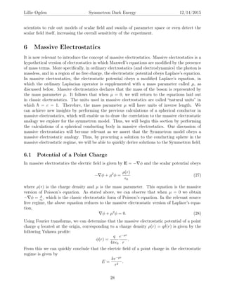
4 Electrostatics and Electrostatic Analogies
Before we begin our exploration of these two scalar field models in greater depth, it is necessary
to explore the heavily understood branch of electrostatics. Electrostatics is a well-explored
area of physics that deals with the phenomena and properties of stationary electric charges
and the resulting electric and magnetic fields. As was shown by Jones-Smith and Ferrer,
electrostatics plays a major role when working with scalar field models of dark energy [9]. In
fact, solutions that are derived from equations in the simple electrostatic regime are relevant to
deftly solve equations that arise in the Chameleon and Symmetron model. Thus, we will begin
by introducing the static regime Maxwell’s equations, which govern the behavior of the electric
and magnetic field. We will then solve the electrostatic equations in the vicinity of a spherical
conductor to find straightforward solutions to Laplace’s equation. We will then introduce the
idea of electrostatic analogies as outlined by Feynman, which are useful in determining solutions
to complex physical phenomena that obey the same mathematical form as Laplace’s equation.
The discussion of electrostatics and electrostatic analogies will enable us to assert that the
Chameleon scalar field obeys an electrostatic analogy, as it obey’s Laplace’s equation. In later
sections, we will introduce a branch of electrostatics called massive electrostatics in order to
declare that the Symmetron obeys a massive electrostatic analogy.
4.1 Electrostatics
Maxwell’s equations are a set of partial differential equations that form the foundation of
classical electrodynamics and electrostatics. They describe how the electric and magnetic fields
are generated and altered by charges and currents, as well as their effect on each other. In the
static regime Maxwell’s equations are as follows
· E =
ρ
0
× E = 0
· B = 0
× B = µ0J.
×E = 0 and ·B = 0 are called the “source free" Maxwell Equations because the 0 on the
right hand side of the equation implies that there is no source from which the field originates.
The source free equations allows us to express the electric and magnetic fields in terms of the
potentials, φ and ξ, at every point in space. However, we are interested in working with the
equations obeyed solely by the electric field. Hemholtz decomposition says that a vector field
can be decomposed into two orthogonal components and expressed as f = φ + × ξ where φ
and ξ are the potentials of the field. Thus, × E = 0, implies that E is completely composed
of an expressive aspect and thus there is no curl of the field. In other words, it is irrotational.
17](https://image.slidesharecdn.com/e63894b1-155e-45af-a04b-329fba2c97ba-160321203613/85/Dark-Energy-Thesis-17-320.jpg)
![Lillie Ogden Symmetron Dark Energy 12/14/2015
4.2 Electrostatic Analogies
The vast amount of information that scientists have discovered about the physical world is
far too large for someone to have gathered even a sensible selection of it. However, people
manage to draw connections and intuitions about the universe that make it drastically simpler
to comprehend the many principles of physics. There are important laws that apply to all types
of phenomena such as the conservation of energy and angular momentum. These quantities and
laws governing the universe limit the possibilities that one could encounter in physics. More
importantly though, the equations for many different physical phenomena have the exact same
mathematical form or appearance. Principles with the same mathematical form of equation
must have the same mathematical form of solution. Thus, identical mathematical forms allow
for a direct translation of the solutions to solve problems in other fields. This is extremely
prevalent in the field of electrostatics, which is outlined in detail by Richard Feynman in The
Feynman Lectures on Physics [10]. Many physical phenomena appear to obey electrostatic
equations in the sense that many physics problems have the form of a potential φ whose gradient
multiplied by a scalar function k has a divergence equal to another scalar function, ρ, ·(k φ) =
ρ. Recalling the discussion of electrostatics, this is simply the general form of Laplace’s equation.
When a physical phenomena obeys Laplace’s equation, it is called an electrostatic analogy. This
enables scientists to quickly derive solutions to more complex situations from the simple case of
electrostatics. Therefore, while learning electrostatics, physicists have simultaneously learned
about a large number of other subjects. Below, we will follow the work outlined by Jones-Smith
and Ferrer to demonstrate how the Chameleon obeys an electrostatic analogy by performing
several calculations and exploring the profile of the field in relevant problems. Next we will
discuss a field of electrostatics called massive electrostatics before investigating the Symmetron
model and arguing that it obeys a massive electrostatic analogy.
5 Chameleon Electrostatic Analogy
The Chameleon Scalar model of dark energy obeys an electrostatic analogy, enabling us to
easily derive solutions in relevant configurations. Under conditions relevant to terrestrial ex-
periments, the Chameleon field obeys the same equations as the electrostatic potential. Recall
that ordinary matter follows the geodesics of
˜gµν = e2βφ/MP l
gµν.
where φ is the Chameleon scalar field. Due to this conformal coupling the effective potential of
the field includes a term that depends on the density of matter, ρm: Veff = V (φ) + A(φ)ρm. In
the Chameleon model, the bare potential V (φ) is non-increasing and A(φ) is non-decreasing.
This results in a minimum for the potential, which is dependent on the presence of ambient
matter density. Recall, that for static configurations of the field, the chameleon obeys 2
φ =
∂Veff
∂φ
. This is called the Klein-Gordon equation. As we mentioned early, this is generally a non-
linear differential equation that is challenging to solve, however, in some regions approximations
allow for relatively simple solutions.
22](https://image.slidesharecdn.com/e63894b1-155e-45af-a04b-329fba2c97ba-160321203613/85/Dark-Energy-Thesis-22-320.jpg)
![Lillie Ogden Symmetron Dark Energy 12/14/2015
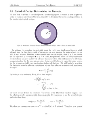
5.1 Field Produced by a Spherical Body
Consider the field produced by a solid sphere of of radius Rc and uniform density ρc immersed
in a uniform background medium [8]. Let us explore the Chameleon profile in the vicinity of
this massive spherical body such as a planet in space, presented in Figure (11).
Figure 11: A solid sphere of of radius Rc and uniform density ρc immersed in a uniform background chameleon gradient.
The conformal coupling establishes that the Chameleon field varies when the density changes.
The sphere is uniformly dense, so the Chameleon field inside the sphere is also uniform, giv-
ing us φ = φc for r < R. Far away, some other density prevails ρ∞ giving rise to a different
chameleon φ∞. As a result, the only place where the chameleon discerns the density contrast is
a thin shell of material just underneath the surface of the sphere. This thin shell of mass is the
only mass that contributes to and sources the outside field. The thin shell suppression factor
is given by
∆Rc
Rc
=
(φ − φ∞)
6βMPlΦc
1,
where ∆Rc is the width of the thin shell and Rc is the radius and Φc is the Newtonian gravi-
tational potential. Virtually all terrestrial objects fall into this thin shell regime, under which
the density contrast is great enough between the inside of the sphere and the boundary of the
sphere so as to make the field inside of the body impenetrable to the field outside of the body.
That is, throughout the core of the spherical body, the Chameleon field rests at the minimum of
Veff , and only the thin shell of matter on the boundary provides a density contrast large enough
to source the Chameleon field outside the body. Thus, the Chameleon field only perceives the
body as r → Rc and only over the course of the thin shell, just underneath the surface, does
the field begin to vary. Once outside the body, the Chameleon is governed by its equation of
motion, 2
φ =
∂Veff
∂φ
. Solving this equation for the spherical body yields
φ(r) ≈
−β
4πMρ,l
3∆Rc
Rc
Mce−m∞(r−Rc)
r
+ φ∞ (22)
This form of solution, (e−λr
)/r, is called the Yukawa profile and under circumstances of interest
23](https://image.slidesharecdn.com/e63894b1-155e-45af-a04b-329fba2c97ba-160321203613/85/Dark-Energy-Thesis-23-320.jpg)
![Lillie Ogden Symmetron Dark Energy 12/14/2015
scalar field φ(r) itself to be very small. Furthermore, the force on a test particle due to the
chameleon field is equally as small since F ∝ φ. This introduces the problem of detection in
the vicinity of spherical bodies, because the force acting on a test mass due to the Chameleon
is adequately small enabling the field to avoid discovery in experiments involving spherical
objects.
5.2 Torque on an Ellipsoid
There is reason to believe that an elliptical test mass could experience an extremely small
torque due to the Chameleon field that experiments would be able to observe. Consequently,
using a solid ellipsoid test mass as a replacement for a solid spherical test mass may allow for
the detection of the Chameleon field in a terrestrial lab. This is permitted due to the concept of
the “lightning rod effect”, that originates from electrostatics. Since the Chameleon field obeys
an electrostatic analogy there is no reason to doubt the presence of the lightning rod effect
in a Chameleon model, and therefore it must be true. In fact it was shown mathematically
by Jones-Smith and Ferrer [9]. Below, we will discuss the lightning rod effect briefly before
examining the behavior of a solid ellipsoid in the presence of a Chameleon field.
5.2.1 Lightning Rod Effect
Figure 12: A depiction of a sphere which has been stretched into an ellipsoid. This object exploits the lightning rod effect as there
is a build-up of charge in regions of high curvature.
Imagine if we stretched the spherical body from Figure(11) into an ellipsoid as in Figure(12).
The lightning rod effect states that the field at the polar region of an elongated object is
enhanced relative to the polar region of a sphere, meaning there are more field lines at the poles
of an ellipsoid than at the equator. This enhancement arises due to the fact that extended
objects such as ellipses have a build-up of charge in regions of high curvature. The build-up of
charge causes a preferred axis for the elongated object in an external field, which the sphere
lacks. This is a general characteristic for of all systems that obey Laplace’s equation and the
boundary conditions that we have assumed here.
25](https://image.slidesharecdn.com/e63894b1-155e-45af-a04b-329fba2c97ba-160321203613/85/Dark-Energy-Thesis-25-320.jpg)
![Lillie Ogden Symmetron Dark Energy 12/14/2015
Figure 13: A conducting ellipsoid immersed in a uniform electric field experiences a torque to align itself with the electric field.
In electrostatics, the electric field at the polar region of a conducting ellipsoid is enhanced
relative to the equator due to build-up of electric charge. If we place a conducting ellipsoid in
a uniform electric field as in Figure(13), a dipole moment forms along the axis of the ellipsoid
and if it is misaligned with the ambient electric field, the ellipsoid will experience a torque in an
attempt to align itself with the electric field. Since the Chameleon is an electrostatic analogy,
we should be able to exploit this effect by calculating the torque on a massive ellipsoid.
5.2.2 Shape Enhancement
Although the thin shell effect of the Chameleon profile arises due to the density contrast and
boundary conditions of a spherical body, it stands to reason that a less symmetric shape would
still possess a thin shell effect. Consider a massive, uniformly dense ellipsoid that is placed into
a uniform Chameleon field gradient [9].
Ellipsoids are three dimensional figures that can be described by prolate spheroidal coordi-
nates (ξ, η, ϕ). ξ = 1/ where is the eccentricity and further, the surface of an ellipsoid has
the radial coordinate ξ = ξ0. η is a measurement of the latitude, where the poles are defined at
η = ±1 and the equator at η = 0. Ellipsoids are convenient objects to work with due to the fact
that they can be compared with spherical results when we impose the limit that the eccentricity
→ 0. It is useful to introduce an equivalent radius Re for the ellipsoid such that the volume
of the ellipsoid is given by 4/3πR3
e. We can assume that the ellipsoid consists of an arbitrary
material and only possesses a thin shell. The interior field value is constant due to the uniform
density of the ellipsoid, ρc, and the exterior field is a solution to Laplace’s equation, since the
Chameleon obeys an electrostatic analogy. We can also define a as the interfocal distance of
the ellipsoid and r as the radial spherical coordinate. Assuming that r >> a, the Chameleon
profile can be written as
φ = φ∞ + f(ξ0)(φc − φ∞)
Re
r
∝
1
r
. (25)
where
f(ξ0) =
2
[ξ(ξ2
0 − 1)]1/3
1
ln[(ξ0 + 1)/(ξ0 − 1)]
(26)
is the shape enhancement factor and we have chosen a = 2Re/[ξ(ξ2
0 − 1)]1/3
. We note that the
ellipsoid has a shape enhancement factor f(ξ0) > 1 that diverges as the ellipsoid flattens to a
26](https://image.slidesharecdn.com/e63894b1-155e-45af-a04b-329fba2c97ba-160321203613/85/Dark-Energy-Thesis-26-320.jpg)
![Lillie Ogden Symmetron Dark Energy 12/14/2015
line. More importantly, this shape enhancement changes the field profile of the Chameleon in
the exterior of the body. We can compare the new field profile in the exterior of an ellipsoid
with the field profile in the exterior of a sphere, where there was unmitigated suppression of the
force imposed on a test mass due to the thin shell effect. If we now use an ellipsoidal source as
opposed to a spherical one, the addition of the shape enhancement factor dominates and is able
to overcome the thin shell suppression factor, which was responsible for causing the Chameleon
to impose an undetectable force on test masses.
Figure 14: A depiction of the lightning rod effect
for a solid sphere which has been stretched into an
ellipsoid. This object exploits the lightning rod ef-
fect as there is a build-up of mass in regions of high
curvature.
Figure 15: A massive, uniformly dense ellipsoid im-
mersed in a uniform Chameleon field gradient ex-
periences a torque to align itself with the ambient
Chameleon field.
Equating this to electrostatics, this is comparable to the lightning rod effect described above.
When a massive, uniformly dense ellipsoid is placed into a uniform Chameleon field gradient as
Figure (15), the shape enhancement factor causes the “charge” to gravitate towards the polar
regions of the ellipsoid, where the curvature is greatest. Instead of a build up of electric charge
in regions of high curvature, there will be a build up of mass at the poles. In other words, the
shell thickness would be enhanced at the poles of the solid ellipsoid, inferring that ellipsoidal
objects would be able to source stronger Chameleon fields. The stronger fields may be able
to overcome the thin shell suppression present in the object, which could lead to a non-zero
force on the solid ellipsoid and a corresponding non-zero torque on the ellipsoid in a Chameleon
field gradient. The fact that a material could cluster in the polar regions of an elongated
object in a Chameleon field gradient is not intuitive but the Chameleon model obeys the same
equations as electrostatics so this must be true as well. So, when we place a uniformly dense
ellipsoid in a uniform chameleon field gradient, a matter dipole moment forms along the major
axis of the ellipsoid and if this dipole moment is misaligned with the ambient field gradient
then it will experience a non-zero torque. Just like an electric dipole can cause a conducting
ellipsoid to torque in an electric field, a matter dipole can cause a solid ellipsoid to torque in a
chameleon field. Simple estimates reveal that the torque is on the order of 10−15
Newton meters.
The central finding is that the chameleon field outside of elongated bodies such as ellipsoids
is enhanced relative to the spherical bodies typically considered in terrestrial experiments [9].
This shape enhancement can be exploited by experimenters to probe new regions of chameleon
parameter space, even in the experimentally unfavorable thin shell regime. This may allow
27](https://image.slidesharecdn.com/e63894b1-155e-45af-a04b-329fba2c97ba-160321203613/85/Dark-Energy-Thesis-27-320.jpg)
![Lillie Ogden Symmetron Dark Energy 12/14/2015
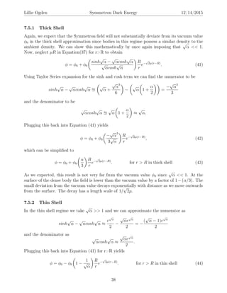
The field begins on the surface of the dense body with value φ/
√
α, which is significantly smaller
than the vacuum value. This is exactly what we saw for the interior profile.
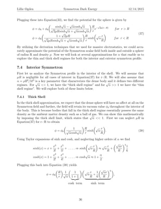
7.6 Symmetron Force in the Exterior Profile
A test particle will experience a force due to the Symmetron field in the exterior of the dense
body. This force could provide experimental relevance when attempting to detect the field. We
will look at the force exerted on the test mass in both then thick and thin shell regime.
7.6.1 Force Analysis: Thick Shell
Assume that we have a test particle of mass m0 placed at a distance r from a dense sphere
of radius R. Also assume that R << r << 1/µ and that the dense body is in the thick shell
regime meaning that
√
α << 1. With these assumptions we find that we can reduce Equation
(43) to
φ ≈ φ0 − φ0
αR
3r
. (45)
Additionally, we can make use of Equation(16) to show that the test particle experiences a force
of
Fφ =
m0φ2
0αR
3M2r2
ˆr. (46)
We can compare this to gravity and show that the ratio of the Symmetron force to the gravi-
tational force is given by
Fφ
Fgrav
= 2
φ0MPl
M2
2
, (47)
where MPl = 1/
√
8πG is the Planck mass and we employed the fact that α = ρR2
/M2
. In a
paper published in 2010, Khoury and Hinterbichler found that gravity and the Symmetron are
comparable in the thick shell regime [11]. Presumably, this is demanded by the Symmetron
field if it is to serve as dark energy. This requirement results in the condition that
φ0MPl
M2
∼ 1. (48)
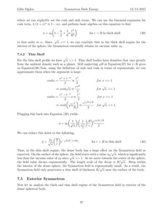
7.6.2 Force Analysis: Thin Shell
Again, assume that we have a test particle of mass m0 placed at a distance r from a dense
sphere of radius R with R << r << 1/µ. Now assume that the dense body is in the thin shell
regime meaning that
√
α >> 1. This simplifies Equation (44) to
φ ≈ φ0 − φ0
R
r
. (49)
The test particle will experience a force of
Fφ =
m0φ2
0R
M2r2
ˆr (50)
39](https://image.slidesharecdn.com/e63894b1-155e-45af-a04b-329fba2c97ba-160321203613/85/Dark-Energy-Thesis-39-320.jpg)
![Lillie Ogden Symmetron Dark Energy 12/14/2015
due to the gradient in the Symmetron field. Again, we can compare this to gravity to find that
Fφ
Fgrav
= 6
φ0Mp
M2
2
1
α
. (51)
We can take into account the condition in Equation(48) to assert that, in the thin shell regime,
the Symmetron force is weaker than the gravitational force by a factor of 1/α. Further, since√
α >> 1, the Symmetron force is much smaller than the gravitational force. Thus we can assert
that tese forces exerted by the Symmetron on a spherical test mass are effectively negligible.
8 Conclusion and Future Work
Modern cosmology aims to study the universe and its complex components. An influx of the-
oretical and experimental astronomers into the field of cosmology coupled with improvement
in observational technology has resulted in an abundance of recent discoveries. The most per-
plexing of these discoveries is the apparent lack of energy density in the universe that many
cosmologists strive to explain by dark energy. This theory attempts to explain the deficient
energy density in the universe, and further, it proposes that this energy is a force working to
counteract gravity and cause the accelerated expansion of the universe. Several classes of models
have been put forth in an effort to understand dark energy. The type of model looked at in this
thesis is a type of quintessence model, which presents dark energy as a slowly evolving scalar
field living in a potential. Several of these scalar fields, such as the Chameleon and Symmetron,
are able to blend in with terrestrial settings, eliminating the potential problems of a generic
scalar field model. Typically, the equations that govern the Chameleon and Symmetron are
involved and cumbersome. However, under conditions of interest on the terrestrial scale, these
equations reduce down to Laplace’s equation, thus representing electrostatic analogies. Exploit-
ing electrostatic analogies when working with dark energy scalar field model simplifies complex
mathematical equations to well understood and manageable forms. For both the Chameleon
and Symmetron models, we find that they both obey Laplace’s equations in the vicinity of a
massive spherical body on terrestrial scales. By utilizing the approach that physical phenomena
described by the same mathematical form of equation possess the same mathematical form, it
is easy to derive valid, insightful profiles for the behavior of these fields.
The Chameleon scalar field was found to obey a classic electrostatic analogy [9]. Thus,
source free, static, and massless electromagnetism provides an analog under which to solve the
Chameleon field in systems of interest. However, for the Symmetron, an unfamiliar and marginal
type of electromagnetism called massive electrostatics seems to provide the analog. We showed
that, although the usefulness of massive electrostatics itself is contentious, the techniques used
to solve problems in the field are nevertheless crucial to solving similar problems with the
Symmetron field. Thus, without the convenience of electrostatic analogies, the solutions to both
the Chameleon and Symmetron scalar fields would be laborious, if not impossible to obtain. It
is also worth noting that these electrostatic analogies are more than a attractive mathematical
trick. These analogies have powerful ramifications with regards to increasing experimental
sensitivity. Scientists hope that we can employ the results obtained from exploring scalar field
models dark energy via electrostatic analogies to either detect the field or rule out its existence
as an explanation for dark energy.
40](https://image.slidesharecdn.com/e63894b1-155e-45af-a04b-329fba2c97ba-160321203613/85/Dark-Energy-Thesis-40-320.jpg)
![Lillie Ogden Symmetron Dark Energy 12/14/2015
The next step will be to calculate the Symmetron profile for an ellipsoidal object to observe
whether it exploits the lightning rod effect. There is no reason to believe that it will not, as it
obey’s Laplace’s equations and maintains similar boundary conditions. It will also be relevant
to calculate the force exerted on a test particle by the Symmetron field in the vicinity of the
polar region of the ellipsoidal object, which we expect to be increased relative to that of a
spherical object. These calculations will enable the exploration into measuring and testing the
Symmetron field itself. The possibility for testing the Chameleon field were made possible after
the calculations performed by Jones-Smith and Ferrer, who introduced the idea that shape
enhancement of elongated objects could probe the Chameleon field [9]. Thus, it is probable
that there exists a similar shape enhancement for the Symmetron field that can be used to
increase experimental sensitivity.
41](https://image.slidesharecdn.com/e63894b1-155e-45af-a04b-329fba2c97ba-160321203613/85/Dark-Energy-Thesis-41-320.jpg)
![Lillie Ogden Symmetron Dark Energy 12/14/2015
References
[1] Hetherington, Norriss S., and W. Patrick McCray.“Cosmic Journey: A History of Scientific
Cosmology.” Center for History of Physics: American Institute of Physics, (2015). Web.
[2] Einstein, Albert. “Kosmologische Betrachtungen zur allgemeinen Relativitätstheorie (Cos-
mological Considerations in the General Theory of Relativity).” Koniglich Preu ische
Akademie der Wissenschaften, Sitzungsberichte (Berlin), (1917): 142-152. Print.
[3] Jones-Smith. “Cosmology Primer”, (2015). Print
[4] “The Expansion of the Universe”. Digital Image. NASA and WMAP.
http://map.gsfc.nasa.gov/universe/uni_fate.html. Web
[5] “The Cosmic Microwave Background Radiation Map”. Digital Image. Physics-
Database.com, (17 Nov, 2012). Web.
[6] Perlmutter, Saul, Brian P. Schmidt, and Adam G. Riess. “Written in the Stars.” The 2011
Nobel Prize in Physics Press Release. Nobelprize.org, (4 Oct. 2011). Web.
[7] High-Z SN search team. Digital Image. http://supernova.lbl.gov/. Nov. 2009. Web.
[8] Khoury, Justin and Amanda Weltman. “Chameleon Cosmology.” Physical Review D. 69.4,
(2004). Print.
[9] Jones-Smith, Katherine and Francesc, Ferrer. “Detecting Chameleon Dark Energy via an
Electrostatic Analogy.” Physical Review Letters. 108.22, (2012). Print
[10] Feynman, Richard P., Robert B. Leighton, and Matthew L. Sands. “Electrostatic Analogs.”
The Feynman Lectures on Physics. Vol. II. Reading, MA: Addison-Wesley Publishing Com-
pany, (1964). Print
[11] K. Hinterbichler and J. Khoury. “Screening Long-Range Forces through Local Symmetry
Restoration”. Phys. Rev. Lett.104, 231301, (2010). Print.
42](https://image.slidesharecdn.com/e63894b1-155e-45af-a04b-329fba2c97ba-160321203613/85/Dark-Energy-Thesis-42-320.jpg)


