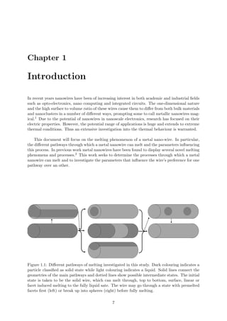
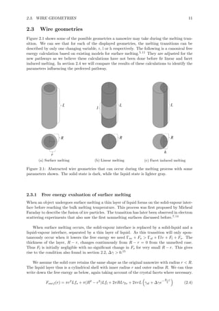
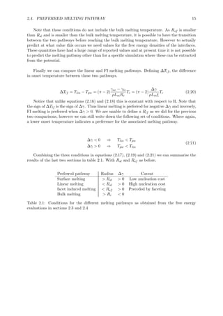
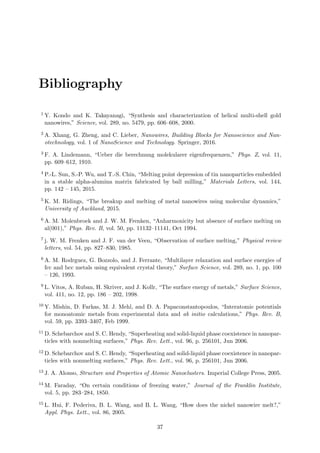
Honours_disertation_Thom_Aldershof

Melting Phenomena in Aluminium Nanowires
Thomas Simon Aldershof
Department of Physics
The University of Auckland
Supervisor: Professor Shaun Hendy
Dissertation submitted in partial fulﬁlment of the requirements for the degree of BSc(Hons) in
Physics, The University of Auckland, 2016.

Abstract
The melting transition of a cylindrical, metal nanowire can progress through a number of differ-
ent pathways. The three pathways identified in this study are surface melting, where a molten
layer envelops a solid core, linear melting, where the wire melts in the longitudinal direction
and fact induced melting, where the wire melts from the surface maintaining at least one solid-
vapour interface. The different pathways are compared both through a simple model based on
free energy considerations, developed here for each pathway, and through molecular dynamics
simulations to identify the main parameters influencing what pathway is taken
From the free energy models, the wire radius and the difference in the energy density of
the different phase interfaces, ∆γ are found as the deciding parameters. A discussion on the
difference in nucleation cost and importance of non-melting crystal facets is also included.
In the simulations, Face Centric Cubic, aluminium nanowires undergo the different melting
pathways using molecular dynamics. From these the radius is confirmed to be an important
parameter deciding between the different pathways. The interface energy of the crystal facets on
the surface of the wire are also identified as important parameters. The latter was accompanied
by shrinkage of the non-melting surfaces through the melting of the wetting surfaces, which the
free energy model does not take account of. The observed melting pathway was also sensitive
to the strength of the coupling of the heat bath, which decided whether the system acts more
canonically or micro-canonically.
The conclusion of this work is that linear melting occurs for wires with a diameter of at most
12 lattice spacings. Surface melting and facet induced melting occurred for thicker wires treated
more canonically or micro-canonically respectively. An accurate theory predicting the onset of
the melting transition needs to take the faceting of the wire into account as the non-melting
surfaces play an important role.
1

Acknowledgements
First and foremost I would like to thank my supervisor Professor Shaun Hendy for suggesting
this subject and allowing me to explore the interesting world of post-graduate research. I would
like to thank him for ensuring the regular meetings were not easily bypassed, even if my results
were meagre. He is also responsible for introducing me to condensed matter through the third
year course he taught together with Associate Professor Malcolm Grimson and Dr. Geoff Will-
mott, who also have my gratitude.
I would further like to thank Dr. Geoff Willmott, as well as Professor Geoff Austin for
introducing me to academic research through the summer research scholarships they offered me
in successive summers.
Next I need to thank Kannan Ridings, who always seemed to be available to answer my
many questions, whether they were technical or theoretical. I am positive he spend more time
on my work than his own on some days and I would like to thank him for this dedication. The
code he provided me at the start of this project allowed me to hit the ground running and
without him this work would be far less complete.
Finally I would like to thank my lecturers, family, friends and peers as they made this year
the most enjoyable, albeit the most demanding year of my university career yet. Special mention
among these is my partner, Rebecca Bub, who always made an effort to help and understand
me in this project and gave her support when I needed it most, whether she was near or far.
3

Contents
Abstract 1
1 Introduction 7
2 Theory 9
2.1 Nucleation Theory . . . . . . . . . . . . . . . . . . . . . . . . . . . . . . . . . . . 9
2.2 Non-melting surfaces. . . . . . . . . . . . . . . . . . . . . . . . . . . . . . . . . . 10
2.3 Wire geometries . . . . . . . . . . . . . . . . . . . . . . . . . . . . . . . . . . . . 11
2.3.1 Free energy evaluation of surface melting . . . . . . . . . . . . . . . . . . 11
2.3.2 Free energy evaluation of linear melting . . . . . . . . . . . . . . . . . . . 12
2.3.3 Free energy evaluation of facet induced melting . . . . . . . . . . . . . . . 13
2.4 Preferred melting pathway . . . . . . . . . . . . . . . . . . . . . . . . . . . . . . . 14
3 Methodologies 17
3.1 Molecular dynamics . . . . . . . . . . . . . . . . . . . . . . . . . . . . . . . . . . 17
3.1.1 Initial state . . . . . . . . . . . . . . . . . . . . . . . . . . . . . . . . . . . 17
3.1.2 Embedded Atom Method Potentials . . . . . . . . . . . . . . . . . . . . . 18
3.2 Numerical considerations . . . . . . . . . . . . . . . . . . . . . . . . . . . . . . . 19
3.2.1 Simulation dimensions . . . . . . . . . . . . . . . . . . . . . . . . . . . . . 19
3.2.2 Time integration and the Langevin thermostat . . . . . . . . . . . . . . . 20
3.3 Post processing . . . . . . . . . . . . . . . . . . . . . . . . . . . . . . . . . . . . . 21
3.3.1 Steinhardt paramaters . . . . . . . . . . . . . . . . . . . . . . . . . . . . . 21
4 Analysis and results 23
4.1 Preliminaries . . . . . . . . . . . . . . . . . . . . . . . . . . . . . . . . . . . . . . 23
4.1.1 Initialistion . . . . . . . . . . . . . . . . . . . . . . . . . . . . . . . . . . . 23
4.1.2 Simulation parameters . . . . . . . . . . . . . . . . . . . . . . . . . . . . . 24
4.2 Observed melting pathways . . . . . . . . . . . . . . . . . . . . . . . . . . . . . . 25
4.2.1 Observation of surface melting . . . . . . . . . . . . . . . . . . . . . . . . 25
4.2.2 Observation of linear melting . . . . . . . . . . . . . . . . . . . . . . . . . 27
4.2.3 Observation of facet induced melting . . . . . . . . . . . . . . . . . . . . . 29
4.3 Comparison to theory . . . . . . . . . . . . . . . . . . . . . . . . . . . . . . . . . 31
5 Discussion 33
6 Conclusions 35
5

Chapter 1
Introduction
In recent years nanowires have been of increasing interest in both academic and industrial fields
such as opto-electronics, nano computing and integrated circuits. The one-dimensional nature
and the high surface to volume ratio of these wires cause them to differ from both bulk materials
and nanoclusters in a number of different ways, prompting some to call metallic nanowires mag-
ical.1 Due to the potential of nanowires in nanoscale electronics, research has focused on their
electric properties. However, the potential range of applications is huge and extends to extreme
thermal conditions. Thus an extensive investigation into the thermal behaviour is warranted.
This document will focus on the melting phenomenon of a metal nano-wire. In particular,
the different pathways through which a metal nanowire can melt and the parameters influencing
this process. In previous work metal nanowires have been found to display several novel melting
phenomena and processes.2 This work seeks to determine the processes through which a metal
nanowire can melt and to investigate the parameters that influence the wire’s preference for one
pathway over an other.
Figure 1.1: Different pathways of melting investigated in this study. Dark colouring indicates a
particle classified as solid state while light colouring indicates a liquid. Solid lines connect the
geometries of the main pathways and dotted lines show possible intermediate states. The initial
state is taken to be the solid wire, which can melt through, top to bottom, surface, linear or
facet induced melting to the fully liquid sate. The wire may go through a state with premelted
facets first (left) or break up into spheres (right) before fully melting.
7

8 CHAPTER 1. INTRODUCTION
The pathways discussed in this document are given by figure 1.1, defining the different melt-
ing geometries encountered. Notice that although the facet pre-melting geometry on the top-left
and the wire break-up on the top-right are encountered in this study, the focus is on the three
melting pathways shown in the centre. Surface melting, where the wire is completely encap-
sulated with a liquid layer. In the linear melting pathway the wire melts in the longitudinal
direction and never becomes fully encapsulated by the melt. Finally, in facet induced melting
the wire melts from the surface but maintains at least one crystal facet as a solid-vapour inter-
face. The final state of the system is always the fully melted case, although it may go through
a geometry where the solid wire has broken up into multiple spheres within the molten wire.
Chapter 2 summarises some of the theory vital to this study. First it revises classical nu-
cleation theory. Then it evaluates how the interface free energy densities influence melting on
different surfaces. With these two elements we then perform free energy evaluations for the
different pathways. At the time of writing we are not aware of a similar evaluation for linear
or facet induced melting in the literature. We then combine these calculations in an attempt
to identify the preferred melting pathway and the parameters influencing this preference. This
again has not been found in literature.
Chapter 3 covers the numerical methods used in this study. The chapter begins with a
discussion of molecular dynamics. This includes a justification of the potential used and lays
out the initial state of the system. It also lists the choices we made to obtain a smooth and
physical simulation that is computationally manageable. Finally it reviews the method used to
distinguish solid and liquid atoms.
Chapter 4 provides an exert of the simulations run showing a representative simulation for
each of the pathways. It also shows the initial state of the system and tests some of the physical
aspects of the simulations. Chapters 5 and 6 provide a summary of our result and point the
way for future research.

Chapter 2
Theory
In this chapter we evaluate some of the theory associated with the melting phenomena and
we attempt to predict the occurrence of the different pathways. We will first review classical
nucleation theory and introduce some relations used in the later sections and then discuss non-
melting facets of a crystal lattice. After this is set-up we engage in a free energy evaluation of
the different melting pathways. This method has been tested for surface melting but is new for
linear and facet induced melting. Finally we compare the relations obtained for the different
pathways to identify parameters that may affect the preference of one melting pathway over the
other.
2.1 Nucleation Theory
An interesting and much-studied aspect of thermodynamics are phase transitions, which is de-
fined as a qualitative change in the properties of an object or material. The most commonly
known examples are melting and vaporisation, the first of which is under discussion in this
document. The onset of this melting transition, as other types of transitions, is described by
classical nucleation theory (CNT).
According to to this theory the melting transition is always initiated at a localised nucleation
site. At this point a stable cluster of liquid needs to be formed from which the melting is then
promoted. One can make the distinction between two types, homogeneous and heterogeneous
nucleation. The former occurs when the nucleation site is within the bulk of the material and
away from any impurity. The latter occurs when the nucleation is encouraged by an impurity of
boundary of the material. In the nanowire, nucleation will always occur on or near the surface
and will thus undergo heterogeneous nucleation.
Both types of nucleation and the following melting transition describe the formation of a
liquid cluster of a certain critical size,l from which the melting transition progresses sponta-
neously. For the nucleation to occur the energetic cost of forming the extra phase interface is
less than the energy gained from the formation of the volume of liquid. Classically the growth
of these nucleation clusters is described by atomic vibrations as first proposed by Lindemann
in 1910. These atomic vibrations increase in amplitude with increasing temperature. However,
this description breaks down for a nanosized object. This is due to the low volume to surface
ratioand thus the relatively high number of less restricted atoms on the surface of the wire.3
9

10 CHAPTER 2. THEORY
The lower energy state results in a depression of the melting temperature of a nano-sized
object. This phenomenon has been extensively verified in the literature for many different
systems and is still an active area of research.2,4 When comparing the liquid and solid state
of a cylindrical nanowire which, for simplicity, maintains its shape and density one can find
section 2.1 for the melting temperature.5
Tm = Tc 1 −
2(γsv − γlv)
ρRLm
(2.1)
Where the temperature dependence was introduced using the relation in equation (2.2). Note
also that the melting temperature is lower than the bulk melting temperature whenever γsv < γlv
.
fs − fl = −ρLm(1 −
T
Tc
) (2.2)
2.2 Non-melting surfaces.
At a nano-scale surface the orientation of the lattice with respect to this surface becomes im-
portant. The direction the surface is cut from the bulk lattice affects a number of properties,
such as the smoothness, packing ratio and surface energy density of the first layer of atoms.
The last of these is of the most interest in this study. In this document, we will specify this
orientation by Miller indices.
The surface energy density is specific to the type of interface the surface is part of. Numer-
ous studies have tried to determine the surface energies of pure metals with varying success.
Experimentally this can often only be found for the solid-vapour energy, γsv, although there is a
large range of reported values. Additionally as the lattice is only present in the solid state, the
liquid-vapour interface, γlv, often has an accepted value independent of the lattice orientation.
However, the solid-liquid interface energy density, γlv, is often difficult to determine as it is
not often a stable state. Even if this is an equilibrium state, atoms will continuously melt and
crystallise and therefore will often not have a well-defined facet. We can define the free energy
density difference.6–10
∆γ = γsv − γsl − γlv (2.3)
This quantity gives the free energy cost of replacing a solid-vapour interface with a solid-
liquid and a liquid-vapour interface per unit area. In other words, the cost to have a layer of
melt form on the solid surface. Like the interfacial energy densities, this quantity depends on
the surface orientation and had been found for some crystal facets of some metals. However,
when ∆γ > 0, a liquid layer will form on this facet and measurements encounter the same
problems as with γsl. In this case ∆γ often can not be determined beyond the negative sign.6
The case where ∆γ > 0 for only some facets of the surface is worth investigating by itself.
As some facets may have this condition satisfied and thus the form a liquid layer (called wetting
surfaces), while others still have positive ∆γ and thus maintain a solid-vapour interface. The
latter quickly gained the name of non-melting surfaces and have been found to cause some in-
teresting phenomena.11–13 In this study, they are important in the occurrence of facet induced
melting, as outlined in section 2.3.3. They also cause the facet melted geometry in figure 1.1.
In Aluminium the (110) facet is a wetting surface, while the (100) and (111) facets are
non-melting surfaces. We thus expect the facet melted geometry to have (110) facets melted
with (100) or (111) intact. Due to the geometry of a nanowire, we cannot have all three facets
as part of the surface.

2.3. WIRE GEOMETRIES 11
2.3 Wire geometries
Figure 2.1 shows some of the possible geometries a nanowire may take during the melting tran-
sition. We can see that for each of the displayed geometries, the melting transitions can be
described by only one changing variable, r, l or h respectively. The following is a canonical free
energy calculation based on existing models for surface melting.5,11 They are adjusted for the
new pathways as we believe these calculations have not been done before fir linear and facet
induced melting. In section 2.4 we will compare the results of these calculations to identify the
parameters influencing the preferred pathway.
(a) Surface melting (b) Linear melting (c) Facet induced melting
Figure 2.1: Abstracted wire geometries that can occur during the melting process with some
parameters shown. The solid state is dark, while the liquid state is lighter gray.
2.3.1 Free energy evaluation of surface melting
When an object undergoes surface melting a thin layer of liquid forms on the solid-vapour inter-
face before reaching the bulk melting temperature. This process was first proposed by Micheal
Faraday to describe the fusion of ice particles. The transition has later been observed in electron
scattering experiments that also saw the first nonmelting surfaces discussed before.7,14
When surface melting occurs, the solid-vapour interface is replaced by a solid-liquid and a
liquid-vapour interface, separated by a thin layer of liquid. As this transition will only spon-
taneously occur when it lowers the free energy we need Γsv + Fs > Γsl + Γlv + Fl + Fs. The
thickness of the layer, R − r, changes continuously from R − r = 0 from the unmelted case.
Thus Fl is initially negligible with no significant change in Fs for very small R − r. This gives
rise to the condition also found in section 2.2, ∆γ > 0.15
We assume the solid core retains the same shape as the original nanowire with radius r < R.
The liquid layer thus is a cylindrical shell with inner radius r and outer radius R. We can thus
write down the free energy as below, again taking account of the crystal facets where necessary.
Fsurf (r) = πr2
Lfs + π(R2
− r2
)Lfl + 2πRLγlv + 2πrL γsl + ∆γe
−R−r
ξ (2.4)

We assume the nanowire to be at equilibrium at all times. This allows us to find the
transition temperature by finding the extrema. Thus we need dF
dr = 0.
dFsurf
dr
= 2πL r (fs − fl) + γls + ∆γ 1 +
r
ξ
e
−R−r
ξ = 0 (2.5)
Where the last term represents the energy cost of nucleation, with ξ, a critical coherence
length of the liquid layer specific to the metal. As before we use equation (2.2) on the unmelted,
initial state, i.e. r = R. Thus we obtain the onset temperature of surface melting, equation (2.6),
in terms of the bulk melting temperature, Tc.
Tsurf = Tc 1 −
γsv − γlv
ρLmR
1 +
R
Rc
(2.6)
Where we defined the critical radius Rc = γsv−γlv
∆γ ξ and used equation (2.3) for ∆γ. It is easy
to see that as long as γsv > γlv and R
Rc
> −1 the onset temperature of surface melting is below
the bulk melting temperature. To ensure this is an energetically stable state we evaluate the
second derivative of the free energy at r = R, T = Tsurf .
d2Fsurf
dr2
= 2πL
∆γ
ξ
R2
+ 2ξ R −
1
2
Rc (2.7)
This is greater than zero for ∆γ > 0 and R > Rc. This ensures that we have been working in
a free energy minimum and surface melting can be an energetically favourable state.
2.3.2 Free energy evaluation of linear melting
Linear melting occurs when a thin cross sectional disk of width l melts before reaching the
bulk melting temperature. As the melting progresses l increases from 0 to L, the length of
the wire. The liquid-vapour interface and the melted volume grow linearly with l as the solid-
vapour interface and solid volume decrease similarly in size. The liquid-solid interface remains
constant and is given by the sum of the two cross sectional areas at either side of the melted disk.
Returning to nucleation theory it is easy to see that this method has a significantly higher
energy barrier than surface melting. Firstly the new interface is mostly away from the sur-
face of the nanowire. This makes the initial nucleation more energy expensive. Secondly this
type of melting does not immediately replace the solid-vapour interface, as we did above and
therefore maintains the, presumably, more expensive interface for longer. We will however still
employ a similar free energy analysis of this pathway. Through similar geometric arguments
as we employed in section 2.3.1 the free energy of the linear melting geometry can be found.
Equation (2.8) gives this as a function of the melting parameter, l.
Flin(l) = πR2
(L − l)fs + πR2
lfl + 2πR(L − l)γsv + 2πRlγlv + 2πR2
γsl + ∆γe
− l
ξ (2.8)
Again the nanowire is assumed to be in an equilibrium state. Finding the minima of the free
energy will thus enable us to find the transition temperature again. Note that this does assume
the nanowire has not undergone surface melting, just as in the previous section we implicitly
assumed the wire had not undergone linear melting.
dFlin
dl
= πR (fl − fs) R + 2 (γlv − γsv) − 2∆γ
R
ξ
e
− l
ξ = 0 (2.9)

2.3. WIRE GEOMETRIES 13
As in the previous section, the last term represents the energy barrier due to the nucleation
process. We again set the wire to the initial, unmelted state, l = 0, to obtain the transition
temperature.
Tlin = Tc 1 − 2
γsv − γlv
ρLmR
1 +
R
Rc
(2.10)
Where Rc = γsv−γlv
∆γ ξ, as before.
Again this transition temperature is below the bulk temperature for γsv > γlv and R
Rc
> −1.
For this to be an energetically accessible state the above parameters need to correspond to a
minimum in the free energy. That is, d2F
dl2 > 0 at l = 0, T = Tlin.
d2Flin
dl2
= 2π∆γ
R2
ξ2
(2.11)
This is greater than zero for ∆γ > 0 and R > Rc. Thus linear melting is an energetically
accessible state.
2.3.3 Free energy evaluation of facet induced melting
Facet induced melting (FI) is an effect of the interplay between wetting and non-melting surfaces.
While the non-melting surfaces of the nanowire remain unmelted, the wetting facets melt. This
allows wetting facet to grow in size. At some point it may be favourable to maintain only
one facet of solid-vapour interface while relinquishing the others in favour of maximizing the
solid-liquid interface of the wetting facets. This geometry is shown in 2.1c. Once again the free
energy can be written down using geometrical arguments.
Fpw(h) = 2RL αRfs +
π
2
− α Rfl + αγsv + (π − α) γlv + α γsl + ∆γe
−2R−h
ξ (2.12)
Where, cos(α) = R−h
R gives half the angle the solid-vapour interface spans.
As in the previous sections the first derivative of the free energy is set to zero to find the minima
of this system. Note that dα
dh = (h(2R − h))−0.5 .
dFpw
dh
=
2RL
h(2R − h)
R(fs − fl) + 2γsl + ∆γ 1 +
2α
ξ
h(2R − h) + 1 e
−2R−h
ξ = 0
(2.13)
We use equation (2.2) to eliminate the volumetric terms and set the system to the onset of
melting, h = R, to obtain the temperature according to this free energy evaluation.
Tpw = Tc 1 − 2
γsv − γls
ρLmR
1 +
π
2
R
Rc
(2.14)
With Rc as in section 2.3.1.
Note that this is less than the bulk melting temperature, Tc, for γsv > γlv and πR
2Rc
> −1 Again
we ensure that the parameters above describe a minimum in the free energy by evaluating the
second derivative with respect to the melting parameter at h = R.
d2Fpw
dh2
= 4
L
ξ
2 + π
R
ξ
∆γ (2.15)
This has the sign of ∆γ and thus we have a minimum for ∆γ > 0. Thus from these free
energy calculations we find that the FI geometry can be an energetically favourable state.

2.4 Preferred melting pathway
In this section we aim to determine the preferred pathway of melting based on the free energy
calculations in the previous section. To do this we will compare the melting temperatures
found in equations (2.6), (2.10) and (2.14). We again ignore the dependence of the surface
energy density on the crystal facet. Otherwise one would use the found values of γsv and ∆γ
for each facet and the facet-independent value for γlv to find the different surface energies. First,
we compare surface and linear melting by defining ∆Tsl, the difference in the onset temperatures
of the two pathways.
∆Tsl = Tsurf − Tlin =
γsv − γlv
ρLmR
1 +
R
Rc
Tc (2.16)
Thus the onset of surface melting precedes the onset of linear melting when equation (2.16)is
negative. As γsv > γlv and R > 0 we deduce that surface melting is preferred when 1 + R
Rc
< 0.
Inversely the linear melting pathway is taken when 1+ R
Rc
> 0. This condition for surface melting
is the inverse of that between surface and the bulk melting temperature, 2.3.1. That is, linear
melting always precedes surface melting according to this canonical calculation. However, due to
the expensive nucleation stage, we can still observe surface melting. This would occur when the
energy cost of nucleation outweighs the energy gain from melting. We can summarise the found
conditions below, while defining the transition radius Rsl, where a lower onset temperature
indicates a preference for this pathway, based on these free energy evaluations.
Rsl = −Rc =
γlv − γsv
∆γ
ξ
R < Rsl ⇒ Tlin < Tsurf < Tc
R > Rsl ⇒ Tc < Tsurf < Tlin
(2.17)
These conditions may be satisfied for some facets of the nanowire while not on the other.
This suggests that surface melting will have its initial nucleation site on a different facet than
linear melting.
We can similarly compare surface melting and FI melting. Defining ∆Tsf , the difference in
the onset temperatures of surface and FI melting.
∆Tsf = Tsurf − Tpw =
γsv − γlv
ρLmR
1 + (π − 1)
R
Rc
Tc (2.18)
The onset of surface melting precedes the onset of FI melting when ∆Tsf < 0. Thus when
1 + (π − 1) R
Rc
< 0 , the wire melts through the surface melting pathway. This now culminates
into the following conditions, defining the transition radius Rsf .
Rsf = −
Rc
π − 1
= −
γsv − γlv
(π − 1)∆γ
ξ
R < Rsf ⇒ Tlin < Tsurf
R > Rsf ⇒ Tsurf < Tlin
(2.19)

2.4. PREFERRED MELTING PATHWAY 15
Note that these conditions do not include the bulk melting temperature. As Rsf is smaller
than Rsl and is smaller than the bulk melting temperature, it is possible to have the transition
between the two pathways before reaching the bulk melting temperature. However to actually
predict at what value this occurs we need values for the free energy densities of the interfaces.
These quantities have had a large range of reported values and at present time it is not possible
to predict the melting pathway other than for a specific simulation where these can be extracted
from the potential.
Finally we can compare the linear and FI melting pathways. Defining ∆Tlf , the difference
in onset temperature between these two pathways.
∆Tlf = Tlin − Tpw = (π − 2)
γsv − γlv
ρLmRc
Tc = (π − 2)
∆γ
ρLmξ
Tc (2.20)
Notice that unlike equations (2.16) and (2.18) this is constant with respect to R. Note that
the sign of ∆Tlf is the sign of ∆γ. Thus linear melting is preferred for negative ∆γ and inversely,
FI melting is preferred when ∆γ > 0. We are unable to define a Rlf as we did for the previous
two comparisons, however we can still write down the following set of conditions. Where again,
a lower onset temperature indicates a preference for the associated melting pathway.
∆γ < 0 ⇒ Tlin < Tpw
∆γ > 0 ⇒ Tpw < Tlin
(2.21)
Combining the three conditions in equations (2.17), (2.19) and (2.21) we can summarise the
results of the last two sections in table 2.1. With Rsl and Rsf as before.
Preferred pathway Radius ∆γ Caveat
Surface melting > Rsl > 0 Low nucleation cost
Linear melting < Rsl > 0 High nucleation cost
facet induced melting < Rsf > 0 Preceded by faceting
Bulk melting > Rc < 0
Table 2.1: Conditions for the different melting pathways as obtained from the free energy
evaluations in sections 2.3 and 2.4

Chapter 3
Methodologies
This section describes the numerical methods used. First, we take a look at molecular dynamics
and the choice of some parameters within this method. We evaluate the elements of a single
simulation to provide reproducibility. This includes a discussion of the computational consider-
ations and simulation parameters. We finish this chapter discussing the Steinhardt parameters
and their role in the solid-liquid classification.
3.1 Molecular dynamics
The model we employed in chapter 2 assumes an approximately cylindrical shape. When the
radius of the wire is sufficiently small, faceting of the nanowire surface renders this assumption
invalid. This puts a lower limit on R, the initial radius of the solid wire. To have a one di-
mensional nano-scale object we need the radius to be less than 100 nm with the length greater
than 100nm. Time integration with a timescale of the order of nanoseconds is required to
have sufficient resolution of the melting process. These constraints fit best within a molecular
dynamics framework. Alternatives would be Monte Carlo or electronic structure methods for
longer timescales or smaller systems respectively.
The first study that can be classified as Molecular Dynamics (MD) was published posthu-
mously by Enrico Fermi.16 The name ”molecular dynamics” was coined by Alder and Wain-
wright 4 years later.17 It is now recognised as an effective method to model many-body systems,
which can be larger and larger as computing power increases, where Fermi started with a mere
64 particles. MD evaluates Newton’s laws on one particle due to a potential created by the
particles in the close environment of this particle. It ignores electronic structure and other
quantum effects, which can be justified by using the Born-Oppenheimer approximation and
assuming that the electrons are in equilibrium with the nucleus.18
3.1.1 Initial state
As outlined in section 3.2 the number of atoms needs to be approximately constant. To obtain
the initial state, these atoms were arranged in an FCC lattice from which we cut a cylinder
along the (100) direction to obtain a nanowire. An example of this initial wire is shown in
figure 3.1.
This wire is placed in a unit cell with periodic boundary conditions in the z-direction such
that we obtain an infinitely long nanowire. We thus eliminate any effects due to the finite length
of the wire and look solely at the nano-dimensions of our wire. For similar reasons there are
solid boundaries in the x and y directions. This ensures there are no interactions in the radial
17

18 CHAPTER 3. METHODOLOGIES
Figure 3.1: Showing the intial state of a nanowire as cut from a perfect FCC lattice. The left
hand figure shows the the (111) plane. The right hand figure faces the (001) plane with the
(100) and (110) planes marked.
direction outside the nanowire.
3.1.2 Embedded Atom Method Potentials
As mentioned before classic MD does not take quantum effects in account. In these methods
intermolecular forces are modelled by hard spheres or more commonly a Lennard-Jones poten-
tial.19 This is radially symmetric, pairwise potential. The equations of motion can now be
obtained from the potential through classical mechanics. Which gives the force between any
pair of atoms as described in equation (3.1). Where the we substituted the Lennard-Jones
potential, ΦLJ .
F(r) = − ΦLJ = 2
rm
r
6
−
rm
r
12
(3.1)
Although the LJ potential is an improvement over the hard sphere model it is still merely a
pair potential model, based only on the inter-atomic separation. The Embedded-Atom Method
(EAM) potentials were developed by Daw and Baskes to model mesoscopic phenomenon such
as micro-fractures in metals. The pair potential had insufficient detail, while methods explicitly
taking electrons into account could not handle the meso scale required.20,21
In EAM methods atoms are embedded into a “Jelium”, that is, they are embedded into
a potential defined not only by the other atoms but also by the electron cloud tied to these
atoms. To avoid solving the Schrödinger equation they assumed that each atom experiences
a locally uniform electron density, defined by the atoms already in the direct environment of
the introduced atom. This electron density is determined empirically. That is, the model is
set up implicitly including this electron density after which it is fitted to experimentally known
parameters. This makes the EAM potentials semi-empirical. It also makes EAM potentials
significantly more accurate than pair potentials while maintaining relatively cheap numerics.
EAM potentials thus need to be tailored to the material under investigation. Furthermore, for
any material there is a number of different potential each suited to a different purpose.22

3.2. NUMERICAL CONSIDERATIONS 19
In this study we investigate phenomena that happen close to the melting point and we thus
hope to model the melting process accurately. For this we need a potential that closely fits the
melting temperature and the latent heat per atom. As these seem to be key parameters from
our study in chapter 2. The potential we chose also accurately models the lattice contraction
or relaxation at the surface. This lattice property can be monitored experimentally through
ion scattering and has been shown to be closely related to the surface energies of the different
crystal facets, another important parameter from our theoretical studies.8,23
All simulations were run on the PAN cluster, maintained by NESI. This allowed us to run
the simulations on parallel cores to maximise the available computing power. The LAMMPS
software, used to run the simulations, quite naturally adopts to parallel computing by dividing
the unit cell into smaller sections. Each of these sections then is assigned to a core. These cores
then only need to communicate about the dynamics close to the box boundaries. LAMMPS
is an open-source software package developed by Sandia National Laboratories and currently
maintained by this institution and Temple University. It is specifically designed for molecular
dynamics and is compatible with the above potential.24
3.2 Numerical considerations
In any numerical simulations one has to make a choice between computational efficiency and
physical completeness. In a simulation one can control almost any aspect of the dynamics,
changing the outcome by changing a single parameter. It is therefore vital that the parameter
set chosen agrees with the physics dominating the real world. One needs to compromise this
absolute accuracy to maintain a simulation with a feasible computing cost. This section dis-
cusses some of the choices this study has made to balance physical accuracy and computing cost.
3.2.1 Simulation dimensions
First among these choices was the size of the initial system already discussed in section 3.1.1.
As outlined in that section a unit cell of any simulation handled in this study contains approxi-
mately 25000 atoms. Note that the EAM potential formally scales as N2 as for any particle the
potential and thus the force on that particle is defined by the positions of all other particles in
the simulation, relative to the particle under consideration. To reduce the computational cost
we only take into account particles that have a significant contribution to this potential, that is
particles in the near neighbourhood of the particle. This near neighbourhood was defined to be
a ball with a radius of 2.5 times the lattice spacing, which is around 10˚Afor Aluminium. The
list of atoms present in this near neighbourhood is updated regularly.
This choice restricts the volume and causes the length and radius of the wire to be directly
related. As the radius is one of the parameters we allow to vary, we should ensure that a
changing length has a minimal impact on the simulated dynamics. Even though our wire is
theoretically infinite, through the periodic boundary condition at the z-boundary, all dynamics
are still contained to just one simulation cell. This is especially worrying for a wire of relatively
large radius, and thus short length as some phenomena may require group dynamics over a
large distance. One of these long range phenomena is the break-up of the molten wire into balls
of liquid to minimise the surface area. This requires the bulk movement of the molten metal
and the momentary increase in surface area as the wire breaks the cylindrical shape. These two
properties make this process a longer wavelength phenomenon and we can use this to test our
system in this respect.

We refer to the wires treated in sections 4.2.1 and 4.2.2 from the results chapter ahead as
the thick and thin wire respectively. The caloric curve of the thin wire shows a rise and fall in
the energy per atom after it has completely molten, corresponding to the break-up of the liquid
wire as discussed above. The caloric curve corresponding to the thicker wire does not show
these dynamics which was some cause of concern. To put these concerns to rest we allowed
the thick wire to continue to heat for half again the simulation time for the thick wire. This
simulation showed a similar dynamic did occur at a higher temperature. The lack hereof in
the regular simulation time could just be due to the fact the thicker wire needs to overcome a
greater energy barrier to break up into the spherical shape. Some confidence that the length
scale is sufficient to capture any melting dynamics can be taken from figure 4.4 where we see
the melting take place at two different sites. This suggest that the wire in that simulation is
significantly longer than the interaction wavelength of any of the melting dynamics.
3.2.2 Time integration and the Langevin thermostat
The next choices concern the time integration of the simulation. Molecular dynamics studies
modelling metals often use a time step of the order of femtoseconds. Any larger than this may
cause discontinuous dynamics where smaller timesteps provide no significant change. In this
particular study we use a timestep of 2 femtoseconds for a million timesteps, giving a total
simulation time of 2 nanoseconds. This simulation length is necessary to capture the complete
melting transition.
To heat the system we use a Langevin thermostat. Physically, the Langevin thermostat can
be thought of as a heat bath of very light solvent molecules in which the system is immersed.
The temperature of this heat bath is controlled exactly. The system attempts to equilibrate
with the heat bath through collisions with the solvent particles. This avoids the system being
treated as a vacuum and allows the temperature of the system to be controlled in a natural
manner through the heat bath. The dynamics for the ith solvent element can be captured by
the following stochastic equation.
mi¨xi(t) = Fi ({x(t)}) −
mi
λi
˙xi(t) + Ri(t) (3.2)
Where mi and xi are the mass and positions of the system particles. Fi is the force de-
fined by the EAM potential, which thus depends on the positions of the nearby particles. R
is a stochastic term with a Gaussian distribution of mean zero. mi
λi
˙x forms the coupling with
the heat bath. The strength of this coupling with respect to the momentum of the particle is
determined by λi, the Langevin parameter, which has units of time and can be seen as the time
necessary for the system to equilibrate with the heat bath. In general this Langevin parameter
can depend on the particle, however in this work it will be constant for all atoms in any given
simulation. Note that the Langevin parameter is inversely proportional to the coupling strength
between the system and the heat bath. Thus a low Langevin parameter will cause the temper-
ature to be strictly controlled by the temperature of the solvent, thus mimicking a canonical
system. Inversely a high Langevin parameters will mimic a micro-canonical system.25,26

3.3. POST PROCESSING 21
3.3 Post processing
During an MD simulation the state of the system is written to files at a fixed time interval.
These files contain the atomic positions, the kinetic and potential energies and the temperature
from the system. The latter two are determined from the velocities of the particles where the
potential is determined by the positions of the atoms within the EAM potential. The energies
and temperature together allow us to plot caloric curves to monitor how the transition differs
from bulk melting.
The atomic positions allow us to make qualitative judgements about the state of the system
and they are instrumental in distinguishing between the different melting pathways. As the
transition progresses a group of atoms changes from being in a strictly ordered lattice to a
disordered, fluid state. This transition is less obvious when looking at a single atom and the
atomic position of one atom is not sufficient to determine the phase this atom is in. However,
we would like to determine whether any atom in our system is part of the solid or liquid phase.
We thus need to evaluate the surroundings of the atom and determine whether it is an ordered
lattice or a disordered fluid.
3.3.1 Steinhardt paramaters
From the many methods in use to do this solid-liquid classification, this study uses the Steinhardt
parameters. These are named after Paul Steinhardt, who published a paper discussing bond
order parameters.27 These are quantities evaluating the symmetry of the ”bonds” around a
particular atom based on spherical harmonics. Here bonds are characterised not only by the
proximity to the atom under consideration but also the direction with respect to other bonds
from this atom. As spherical harmonics are distinguished by their degree, l, there are different
degrees of the Steinhardt parameters, denoted ql. In this study only the order parameter of the
sixth degree is of interest.
Figure 3.2: Snapshots showing the progression with a consistent solid-liquid distribution in
cross-section throughout the length of the wire with atoms classified as either solid (copper)
or liquid (blue). Each snapshot is accompanied by the distribution of the ¯q6 Steinhardt order
parameter for that frame showing the classification as either solid (green) or liquid (blue).
Together they form an empirical confirmation of the validity of the Steinhardt parameters as
a method for solid-liquid classification. The last snapshot has all atoms classified as liquid
removed, to highlight a shortcoming of this method.

The Steinhardt parameters can thus be used to distinguish between different lattice types as
well as between the solid and liquid state. Locally this is captured by a complex valued vector
for each atom describing the length and direction of each bond to this atom. This vector can be
converted to real numbers by taking the Fourier invariant of the field of neighbouring complex
vectors. Finally these are averaged to smoothen the distribution of thermal fluctuations. These
average values are denoted as ¯ql, where we use the ¯q6 order parameter in this study.27,28
Thus in short the Steinhardt parameters are real values assigned to each atom quantifying
the relation this atom has to its neighbourhood. The values of these ¯q6 corresponding to dif-
ferent crystal structures and thermodynamic phases can be found in literature. The latter of
these makes these parameters useful in following a phase transition. It is worth noting that we
need to define a radius of the near neighbourhood of an atom, for this method of liquid-solid
classification to function. This distance is usually chosen to be the first minimum of the ra-
dial distribution function, which can be found either from the atomic positions or the literature.
To test the solid-liquid classification we’ve picked a simulation that had a fairly consistent
cross-sectional picture. In other words, for any particular frame, the image seen for the cross-
sectional snapshot does not change significantly as the viewpoint moves along the length of the
wire. For such a wire the proportion of liquid to solid atoms in the cross-sectional snapshot
should be approximately the same as that proportion for the complete wire. Representative
snapshots of these cross sections are shown in figure 3.2 along with the distribution of the ¯q6
parameter for the wire at the time of that snapshot.
We can now visually confirm that the atoms classified as liquid, actually seem to be in a
disordered state. Similarly, the atoms classified as solid are ordered into a crystal lattice. Some
small calculations also give that the distribution of the ¯q6 parameter gives the same liquid frac-
tion as counting the atoms in a representative number of layers in the cross-sectional snapshot.
However the last snapshot shows a seemingly fully melted wire with some atoms classified as
solid still present along the surface of the wire. These atoms appear to be misclassified due to
their position at the physical boundary of the system. Aside from this caveat, we believe the
Steinhardt order parameter to be a valid method of solid-liquid classification.

Chapter 4
Analysis and results
In molecular dynamics the position of all atoms can be tracked throughout the simulation.
This allows us to take snapshots at any given time to evaluate the state of the system. Exam-
ples of these snapshots can be found throughout this chapter. This becomes especially useful
after solid-liquid classification as discussed in section 3.3. In these simulation it was chosen
to take snapshots every 4000 fs and thus produce 500 snapshots for a 2ns simulation. With
these snapshots we also evaluate the temperature, from the average speed of the particles, as
well as the kinetic and potential energies of the system and per atom. Where the energies are
found from average speeds and the positions of the atom within the EAM potential respectively.
We can use all this information to evaluate our simulations in a more qualitative manner.
In this chapter there are two main parameters that are varied. The first is the size of nanowire,
defined by its radius. The total length is trivially held constant through the periodic boundary
condition in the z-direction and is thus not a relevant parameter. Note that the length of the
wire within a unit cell may change between simulations, as described in section 3.2.1.
4.1 Preliminaries
Before running the simulations of wires along the different melting pathways we need to en-
sure that our simulations model a physical and stable system. We first ensure that the initial
system is a stable and feasible configuration We also check the simulation parameters such as
the Langevin parameter and the heating rate are within a reasonable range and provide the
required resolution to monitor the changing system. Finally we explore some of the output
parameters and visualisation tools available. This include verifying the Steinhard parameter
accurately classifies solid and liquid atoms.
4.1.1 Initialistion
As discussed in chapter 3 we first need to equilibrate the wire and allow the lattice to relax.
To allow this we performed an NVT minimisation before starting each simulation. We notice
a slight, but important change in the wire geometry after this relaxation period. Figure 4.1
shows a (001) cross-sectional view of the initial wire before and after relaxation at 600 Kelvin,
the initial temperature of our simulations. To ensure that the right hand side was a stable state
a simulation was run unheated for the length of the later simulations, 2 ns. This preserved the
shape of the wire sufficiently and no un-physical behaviour was noticed.
23

24 CHAPTER 4. ANALYSIS AND RESULTS
We can see that before the relaxation period the wire is cut from a perfect lattice, as none
but the first layer of atoms are visible. Although the cross section is not perfectly circular, the
layering of the atoms is such that it models this shape as closely as possible. This perfection
disappears after relaxation. First we note the slight thermal expansion. We also see the atoms
that were hidden behind the first layer due to the stochastic elements of the potential and the
non-uniform initial velocity distribution. However, the wire still has a distinct crystal structure,
which is re-established by the fact that almost all atoms are still classified as solid. The few
atoms classified as liquid can be seen as outliers that will likely soon crystallise again.
A more subtle effect of the relaxation is the increased faceting of the cross section. We
see that in particular the diagonal facets have flattened as to maximize the (110) facets. This
results in the cross section becoming almost octagonal with the (110) and (100) facets being
the only two substantial facets on the surface of the wire. This is likely to have an effect as
chapter 2 found the surface energies of these facets to be critical. We still expect the theory to
hold reasonably well as we knew the perfectly cylindrical shape was an approximation in that
chapter.
4.1.2 Simulation parameters
As outlined in section 3.2 the total heating done and the total duration of the simulations is
held constant. It seems to follow that the heating rate remains constant across simulations.
This only holds true for the heat bath connected to our simulation. The Langevin parameter,
λ, influences the rate at which this heat enters the nanowire system. As this parameter is the
means to control what ensemble the simulation represents we cannot avoid this discrepancy.
Instead we will investigate the influence of the Langevin parameter on the heating rate.
Figure 4.1: Initial wire as created before the start of the simulation (left) and after an initial
relaxation period (right) with the crystal facets indicated. Atoms classified as solid are indicated
copper while those classified as liquid are blue.

4.2. OBSERVED MELTING PATHWAYS 25
4.2 Observed melting pathways
In this section the different pathways outlined in the theory of chapter 2 are found and followed
in simulation. We managed to find each of the pathways discussed in the theory and will thus
discuss them again and compare the theory to the simulations.
4.2.1 Observation of surface melting
As described in section 2.3.1, surface melting is the forming of a liquid layer on the nanowire
surface. This liquid layer encapsulates the remaining solid core fully for there to be complete
surface melting. Figure 4.2 shows the progression of the transition through snapshots. Fig-
ure 4.3 shows the caloric curve and liquid fractions of two simulations showing surface melting
at different Langevin parameters. The left graph is of the same simulation as the snapshots.
Note that the actual melting transition is relatively short. It is preceded and followed by a
significant heating period characterised by a linear trend in the caloric curve. This shows the
wire is a physical and stable system.
Figure 4.2: Snapshots for the progression of surface melting left to right, top to bottom. This
simulation has a relatively thick wire and low Langevin parameter λ = 10ps. Atoms identified
as solid are copper coloured, blue indicates atoms in a liquid state. Each snapshots has 4
projections of the wire, two side on views, facing the (110) plane(left) and two cross sections,
facing the (001) plane(right). The top row shows the full wire where the bottom row shows
only the atoms classified as solid.

We can now compare the snapshots with the caloric curve through the liquid fraction. Each
snapshot has 4 projections of the wire as outlined in the caption. First note that snapshot A
is not the initial state of the wire, which looks more like figure 3.1. Snapshot A is just before
the onset of surface melting. We see that the (110) facets have already melted and now form a
solid-liquid interface. These facets have increased in size by melting the sides of the (100) facets,
which are also part of the (110) facet. This period of facet melting can be seen as a relatively
slow, but accelerating rise of the liquid-solid fraction to about 10 percent. At the same time
we see the caloric curve deviating from the linear heating characteristic for a fully solid system.
This is due to the transition of these atoms from solid and liquid and the associated latent heat.
Snapshot B shows the wire just after the onset of surface melting. We see the wire fully
encapsulated in a liquid layer with solid core tending to maximise the (110)-facets. This is
reinforced in snapshot C which shows the same wire at a later stage of surface melting. Keep in
mind that all atoms are displayed in these snapshots, gradually fading as they are further away.
Thus although in snapshot C there seems to be a significant (100) facet on the right hand side of
the wire, especially obvious in the solid only cross section. However, it is quite thin and we see
that there is a second facet further towards the centre where we see a far greater density of the
displayed atoms, showing that this later facet extends along a larger portion of the wire. The
melting of the solid core also seems to be fairly symmetric, allowing the solid core to remain
in the centre. This is backed up by the linear trend in the liquid fraction between 10 and 90
per. We see this corresponds to the flat section in the caloric curve, as one would expect from
a canonical system.
The final snapshot, D, shows the wire after the solid core has broken up and there is only
a small cluster remaining. This cluster would melt away quickly as it contains less than 10
percent of the original atoms. We see that the liquid fraction flattens again as the number
of solid atoms remaining becomes of the order of misclassified atoms near the surface. After
the liquid fraction reaches this maximum value the caloric curve again assumes a linear trend,
showing the heating of a pure liquid.
The second graph in figure 4.3 shows the caloric curve and liquid fraction for the same wire
in a simulation with a higher Langevin parameter. These follow a very similar trend as do the
snapshots, hence why these are not shown. However, the caloric curve starts to show a definite
dip in temperature, after reaching a maximum. This shows the changing ensemble as we move
away from the canonical treatment. When the Langevin parameter further we start to see facet
induced melting. This is discussed further in section 4.2.3.
Figure 4.3: Caloric curves (red) with liquid fraction (blue) for a simulation of surface melting.
These simulations have different Langevin paramaters, λ = 10ps and λ = 40ps, respectively.

4.2.2 Observation of linear melting
Similar to the previous section figure 4.4 shows the progression of linear melting in snapshots
while figure 4.5 shows the caloric curve and liquid fraction of two different simulations showing
linear melting. The snapshots are for a simulation with Langevin parameter λ = 200ps. Thus
the right caloric curve corresponds to the same simulations as the snapshots. This particular
value was chosen because the snapshots obtained from this simulation best showed the range
of phenomena encountered. Linear melting was observed for the full range of the Langevin
parameter. In other words for both canonical and micro-canonical systems. Note that this is
not true for surface melting or for facet induced melting in thicker wires, as we will encounter in
the next section. As before the actual melting transition is a relatively small part of the caloric
curve, to ensure the system is physical. At the end of the caloric curve we see the forming of a
liquid ball and the associated drop in energy, as discussed in section 3.2.
First we examine the snapshots. The first thing to note that the wire needed to be signif-
Figure 4.4: Snapshots showing the progression of linear melting left to right, top to bottom.
This simulation has a relatively thin wire and an intermediate Langevin parameter λ = 100ps.
Atoms identified as solid are copper coloured, blue indicates atoms in a liquid state. Each
snapshots has 4 projections of the wire, two side on views, facing the (110) plane(left) and two
cross sections, facing the (001) plane(right). The top row shows the full wire where the bottom
row shows only the atoms classified as solid.

icantly thinner to clearly and reliably show linear melting. This agrees with what we saw in
chapter 2 where the distinguishing feature between linear and surface melting seemed to be the
radius, Rsl. However a caveat was placed by this finding as linear melting has a significantly
higher nucleation cost and thus may not be preferred when close to this critical radius. This is
reflected in snapshot A, which again is not the initial state, where a significant portion of the
atoms have already melted but the wire still has not cut through. The energy cost in the latent
heat of these atoms is related to the nucleation cost of this pathway.
In most snapshots we see some faceting is present in the cross-section of the full wire. How-
ever, it is significantly less strong and from the solid only pictures we see that the faceting
only occurs along sections of the wire as these cross-sections remains fairly round for the full
duration of simulation. Snapshot B shows the wire just after it has been cut through and we
see that it seems to be cut in two places, one just out of view at the left. The lower section
in between these cuts is also completely detached from the lower surface. I.e. it is undergoing
facet-induced melting. This is reinforced by snapshot C, which also shows this part of the wire
has melted significantly faster, which is partly due to the smaller size in snapshot B and partly
due to the greater melting surface for facet induced melting.
The fact that we see these two different pathways supports the hypothesis that the nucle-
ation cost of linear melting is an important factor. Since nucleation is ultimately a random
process, it is to be expected that we see seemingly ambiguous results as figure 4.4. When we
compare the snapshots with the right-hand liquid fraction we see this reflected as a kink be-
tween two fairly linear trends. This kink is the moment the facet induced melting has finished
and we are left with only linear melting. The initial nucleation is reflected in the initial curved
section, which now does not represent faceting. We see a similar trend in the caloric curve.
initially there is a linear trend as we are heating a pure solid. When the liquid fraction starts to
increase, the caloric curve deviates from this linear trend. In the period with the two melting
types simultaneous we see a sharp drop in te caloric curve as energy is released as latent heat
faster than the system is allowed to heat up under this high Langevin parameter. After the
facet induced melting is completed the temperature slowly increases again as the latent heat of
the linear melting alone is not enough to maintain the negative gradient.
The linear melting pathway was observed only for relatively thin wires, with a diameter of
at most 12 lattice spacings. However, when linear melting seems largely independent of the
Langevin parameter. When linear melting was observed for a simulation with low λ it would
generally also been seen for a simulation with λ large.
Figure 4.5: Caloric curves (red) with liquid fraction (blue) for a simulation of linear melting.
These simulations have different Langevin paramaters, λ = 10ps and λ = 200ps, respectively.

4.2.3 Observation of facet induced melting
As in the previous two sections the snapshots shown in figure 4.6 and the caloric curve and liquid
fraction found in figure 4.7 follow a nanowire undergoing facet induced melting. The snapshots
are for a simulation with a high Langevin parameter, λ = 200ps. Thus the corresponding caloric
curve is on the right. Unlike what was observed for the linear melting pathway, the Langevin
parameter needs to be sufficiently high to observe facet induced melting. In other words, we
observe it only for more micro-canonical systems.
In section 2.3.3 we defined facet induced melting (FI) as a melting transition that forms a
liquid layer on most of the surface while maintaining a solid-vapour interface on at least one
facet for the duration of the transition. This is indeed what we see in the snapshots below.
In snapshot A there significant faceting occurs along the full length of the wire. However, the
faceting is not symmetric as it was for surface melting. Only the (110) facets on the right
hand side have melted along the full side of the wire. This asymmetry was present in all FI-
simulations, even though it seemed random which side of the wire would melt.
Note that the side-on view has been rotated from the cross section such that the right hand
Figure 4.6: Snapshots for the progression of facet induced melting left to right, top to bottom.
This simulation has a relatively thick wire and high Langevin parameter λ = 200ps. Atoms
identified as solid are copper coloured, blue indicates atoms in a liquid state. Each snapshots
has 4 projections of the wire, two side on views, facing the (110) plane(left) and two cross
sections, facing the (001) plane(right). The top row shows the full wire where the bottom row
shows only the atoms classified as solid.

side, the side showing the initial melting, faces towards the viewer. Snapshot B shows the same
asymmetry. The wire has now completely disconnected from both the (110) and (100) facets
on the right hand side of the cross-sections. Examining the side-on view, we see that the solid
phase still extends the full width of the wire. There is still a significant fraction of these (110)
facets that maintains a solid-vapour interface. This part resembles the geometry used in the
chapter 2, but the rest of the wire does not. Showing an almost spherical shape, flattened by
last remaining (110) solid-vapour interface. Recall that in the chapter 2 we did not properly
take account of the wetting and NM facets, which is likely to be the source of this discrepancy
between the theory and simulation.
The liquid fraction follows a fairly un-eventful trend looking a lot like that for surface melt-
ing. We initially see the initial melting of the (110) facets in the almost quadratic increase in
liquid fraction. As the wire starts the main melting process after forming the liquid layer on the
(100) facet the liquid fraction follows a linear trend, which continues until a near 100 percent
liquid fraction is reached. The caloric curve however is slightly different showing a definite dip in
temperature as the melting progresses. This is again explained by the high Langevin parameter.
This makes the transition occur in a more micro-canonical ensemble. Thus the kinetic energy
of the atoms, inseparable from the temperature, is used directly to supply the heat required for
the melting transition rather than the heat added to the system through the heat bath.
Snapshot C shows the wire after a period of FI melting. The solid remainder is now dis-
connected from all of the wire surface except for the (100) facet on the far side of the side-on
view. Based on cross section, it seems there is still strong faceting present, despite the constant
melting at the solid-liquid interface. Snapshot C also shows the wire as it is about to break up.
Notice that the break-up occurs for a significantly thicker wire than seen for surface melting
earlier. After the break-up the solid remainder is melted while still maintaining a solid-liquid
frame all the way to snapshot D, which was one of the last frames before the completely molten
state.
The FI pathway was observed for wires of the same radius as those for surface melting, but
at a significantly higher Langevin parameter, generally with λ > 100ps. When the radius of the
wire was made smaller this pathway is no longer preferred over linear melting and we no longer
see the facet induced melting pathway.
Figure 4.7: Caloric curves (red) with liquid fraction (blue) for a simulation of facet induced
melting. These simulations have different Langevin paramaters, λ = 120ps and λ = 200ps,
respectively.

4.3. COMPARISON TO THEORY 31
4.3 Comparison to theory
The simulations discussed in this chapter have managed to reproduce each of the pathways dis-
cussed in chapter 2. We identified some of the parameters governing which pathway is observed.
The parameters found in this chapter are summarised in table 4.1. This section will evaluate
the agreement between the two approaches and discuss the differences.
Preferred pathway Radius Langevin parameter, λ Caveat
Surface melting > 8a < 40 Shrinkage of Non-melting surfaces
Linear melting < 6a > 0, < 200 No pre-melting facets
facet induced melting > 8a > 80 Preceded by assymetric faceting
Bulk melting - - Not invesigated in this chapter
Table 4.1: Conditions for the different melting pathways as observed in molecular dynamics
simulations. The lattice parameter, a is 4.050˚Afor FCC aluminium.
Note that the conditions on the radius and Langevin parameter are not closely fitting. In
between these boundary values we would often observe a strong competition between two path-
ways. Some examples of which are included in figure 4.8. The competition between linear and
facet induced melting was already shown in figure 4.4.
The deciding parameter between linear melting and both surface and facet induced melting
seems to be the radius, as we found only for the former of these comparisons in the free energy
evaluation. From table 4.1, one is tempted to estimate Rsl to be between 6 and 8 lattice spacings.
However, we have not been able to identify the nucleation cost of the different pathways, and
closer investigation may reveal a higher critical radius. We have not been able to identify the
surface energy as an explicit parameter but have seen the important role of the crystal facets
and the Langevin parameter. These findings suggest that for facet induced melting the simple
model employed in chapter 2 is not sufficient.
Figure 4.8: Two examples of competing pathways, with atoms classified as solid (liquid) shown
in copper (blue). Snapshot A show part of the wire surrounded by melt while the other half
of the wire attempts to maintain a solid-vapour interface, showing the competition between
surface and facet induced melting. Snapshot B shows competition between surface and linear
melting as the solid phase becomes fully encapsulated in the melt after a cross-sectional cut.

Chapter 5
Discussion
In this study we investigated three different pathways through which a nanowire can melt.
Chapter 2 compared the pathways by means of a free energy evaluation, calculating the free
energy cost and predicting a melting temperature for each wire. This approach made a number
of approximations which overlooked possibly important details. Foremost among these was the
shape of the nanowire. As we assume a cylindrical shape the faceting seen in the simulations
is not taken account of. This is vital in predicting the melting temperature as this depends
heavily on the phase interface energy densities. These energy densities depend on the crystal
facet at which the interface is located.
A more complete investigation may be made when an octagonal cylinder is assumed. The
sides of the octogonal can then be taken to be the different crystal facets and one may acquire an
expression for the temperature in terms of the specific interface energies of the different facets.
Allowing experimental or simulation parameters to be substituted to predict the melting tem-
perature and pathway of a given wire. The cross section may also be allowed to change into
an irregular octagonal by letting the wetting surface to melt the sides of non melting surfaces.
This would make for significantly more complicated expressions but would model a number of
the interesting phenomena encountered in simulation more closely.
Another source of discrepancy between theory and simulation originated from ignoring the
nucleation cost of the different pathways. Based on the free energy evaluation in chapter 2 the
linear pathway is always preferred below the bulk melting temperature. However, in chapter 4
we certainly saw both pathways. This is likely due to the linear melting transition needing to
overcome a greater energy barrier in the nucleation stage during which the simulation is still
heated. Thus if this barrier cannot be overcome before reaching a temperature at which surface
melting is possible we may see either pathway.
Future work may simulate wires with a differently orientated lattice. Of special interest
would be a wire with only (110) and (111) facets which should highlight any difference between
the two non-melting facets in Aluminium, after the (100) facet was examined here. Another
interesting case would be a geometry with only the non-melting surfaces (111) and (100) at the
surface, although this is not possible in a cylindrical nanowire.
It should also be noted that this study observed multiple wires in which more than one
pathway was followed. This co-occurrence of two pathways may be of interest to another study
as it changed the stability of the solid significantly, often melting significantly quicker in the
boundary areas. An example of co-occurrence of linear and facet induced melting is given in
section 4.2.2.
33

34 CHAPTER 5. DISCUSSION
Finally future studies could investigate similar behaviour for nanowires consisting of differ-
ent materials. The authors believe that any FCC metal with two non-melting surfaces should
behave qualitatively similar to the aluminium studied here. However, a metal with a different
crystal lattice or an FCC lattice with one or zero non-melting surfaces may behave quite differ-
ently.

Chapter 6
Conclusions
Simulations using molecular dynamics were carried out to investigate melting phenomena in
metal nanowires. The main focus was on the different pathways through which a nanowire can
melt. In this study surface melting was observed for wires with relatively large radius in canoni-
cal simulations. Facet induced melting was observed for similar wires treated micro-canonically.
Linear melting was observed for both canonical and micro-canonical systems for wires with
a diameter smaller than 12 lattice spacings, where the system ensemble was decided by the
Langevin parameter, λ.
Another melting phenomena investigated, albeit less in-depth, was the faceting in melting
due to the presence of both wetting and non-melting facets at the nanowire surface. The pres-
ence of this state before the system seems to be associated with the melting pathway taken.
This state was not significantly present before linear melting, while the facets melt symmetri-
cally for surface melting and showed asymmetry for the facet induced melting.
An attempt was made to explain and predict the pathways using free energy evaluations for
a simple model of a nanowire. This managed to predict the dependence of the melting pathway
on the radius of the wire and the importance of the interface energy difference, ∆γ. However it
was discovered that an accurate theory describing these phenomena needs to take the faceting
dynamics and the cost of nucleation into account.
This work thus identified three different pathways for the melting transition in a nanowire.
It also identified some of the main parameters influencing the pathway taken by any particular
wire. This work is of importance as electronic components reach the nanoscale and are pushed
to their thermodynamic limits. Future research directions are outlined in chapter 5.
35

Bibliography
1 Y. Kondo and K. Takayanagi, “Synthesis and characterization of helical multi-shell gold
nanowires,” Science, vol. 289, no. 5479, pp. 606–608, 2000.
2 A. Xhang, G. Zheng, and C. Lieber, Nanowires, Building Blocks for Nanoscience and Nan-
otechnology, vol. 1 of NanoScience and Technology. Springer, 2016.
3 F. A. Lindemann, “Ueber die berechnung molekularer eigenfrequenzen,” Phys. Z, vol. 11,
pp. 609–612, 1910.
4 P.-L. Sun, S.-P. Wu, and T.-S. Chin, “Melting point depression of tin nanoparticles embedded
in a stable alpha-alumina matrix fabricated by ball milling,” Materials Letters, vol. 144,
pp. 142 – 145, 2015.
5 K. M. Ridings, “The breakup and melting of metal nanowires using molecular dynamics,”
University of Auckland, 2015.
6 A. M. Molenbroek and J. W. M. Frenken, “Anharmonicity but absence of surface melting on
al(001),” Phys. Rev. B, vol. 50, pp. 11132–11141, Oct 1994.
7 j. W. M. Frenken and J. F. van der Veen, “Observation of surface melting,” Physical review
letters, vol. 54, pp. 827–830, 1985.
8 A. M. Rodrguez, G. Bozzolo, and J. Ferrante, “Multilayer relaxation and surface energies of
fcc and bcc metals using equivalent crystal theory,” Surface Science, vol. 289, no. 1, pp. 100
– 126, 1993.
9 L. Vitos, A. Ruban, H. Skriver, and J. Kollr, “The surface energy of metals,” Surface Science,
vol. 411, no. 12, pp. 186 – 202, 1998.
10 Y. Mishin, D. Farkas, M. J. Mehl, and D. A. Papaconstantopoulos, “Interatomic potentials
for monoatomic metals from experimental data and ab initio calculations,” Phys. Rev. B,
vol. 59, pp. 3393–3407, Feb 1999.
11 D. Schebarchov and S. C. Hendy, “Superheating and solid-liquid phase coexistence in nanopar-
ticles with nonmelting surfaces,” Phys. Rev. Lett., vol. 96, p. 256101, Jun 2006.
12 D. Schebarchov and S. C. Hendy, “Superheating and solid-liquid phase coexistence in nanopar-
ticles with nonmelting surfaces,” Phys. Rev. Lett., vol. 96, p. 256101, Jun 2006.
13 J. A. Alonso, Structure and Properties of Atomic Nanoclusters. Imperial College Press, 2005.
14 M. Faraday, “On certain conditions of freezing water,” Journal of the Franklin Institute,
vol. 5, pp. 283–284, 1850.
15 L. Hui, F. Pederiva, B. L. Wang, and B. L. Wang, “How does the nickel nanowire melt?,”
Appl. Phys. Lett., vol. 86, 2005.
37

38 BIBLIOGRAPHY
16 E. Fermi, J. Pasta, S. Ulam, and M. Tsingou, “Studies of nonlinear problems,” Los Alamos,
1955.
17 B. Alder and T. Wainwright, “Studies in molecular dynamics. i. general method,” The Journal
of Chemical Physics, pp. 459 – 466, 1959.
18 D. Frenkel and B. Smit, Understanding Molecular Simulations: from algorithms to applica-
tions. Computational sciences series, Academic Press, Hartcourt, 2002.
19 J. E. Jones, “On the determination of molecular ﬁelds. ii. from the equation of state of a
gas,” Proceedings of the Royal Society of London A: Mathematical, Physical and Engineering
Sciences, vol. 106, no. 738, pp. 463–477, 1924.
20 M. S. Daw and M. I. Baskes, “Semiempirical, quantum mechanical calculation of hydrogen
embrittlement in metals,” Phys. Rev. Lett., vol. 50, pp. 1285–1288, Apr 1983.
21 M. S. Daw and M. I. Baskes, “Embedded-atom method: Derivation and application to im-
purities, surfaces, and other defects in metals,” Phys. Rev. B, vol. 29, pp. 6443–6453, Jun
1984.
22 M. S. Daw, S. M. Foiles, and M. I. Baskes, “The embedded-atom method: a review of theory
and applications,” Materials Science Reports, pp. 251–310, 1993.
23 Y. Mishin, D. Farkas, M. J. Mehl, and D. A. Papaconstantopoulos, “Interatomic potentials
for monoatomic metals from experimental data and ab initio calculations,” Phys. Rev. B,
vol. 59, pp. 3393–3407, Feb 1999.
24 S. Plimpton, “Fast parallel algorithms for short-range molecular dynamics,” Journal of Com-
putational Physics, vol. 117, no. 1, pp. 1 – 19, 1995.
25 T. Schneider and E. Stoll, “Molecular-dynamics study of a three-dimensional one-component
model for distortive phase transitions,” Phys. Rev. B, vol. 17, pp. 1302–1322, Feb 1978.
26 I. Snook, The Langevin and Generalised Langevin Approach to the Dynamics of Atomic,
Polymeric and Colloidal Systems. Amsterdam: Elsevier, 2007.
27 P. J. Steinhardt, D. R. Nelson, and M. Ronchetti, “Bond-orientational order in liquids and
glasses,” Phys. Rev. B, vol. 28, pp. 784–805, Jul 1983.
28 A. S. Keys, C. R. Iacovella, and S. C. Glotzer, “Characterizing structure through shape
matching and applications to self-assembly,” Annual Review of Condensed Matter Physics,
pp. 263–285, March 2011.

Honours_disertation_Thom_Aldershof

More Related Content

Viewers also liked

Similar to Honours_disertation_Thom_Aldershof

Honours_disertation_Thom_Aldershof