02. Fracking the Ohio RiverAnalyzing the Risk of Induced Seismicity Introduction and Background This is the second in our series of homeworks focused on evaluating geohazard risks in the vicinity of the Ohio River between Washington Couty, Ohio and Pleasangs Couty West . In this assignment we will appraise whether or not this area shows any potential risk of earthquakes from a plan by the state of West Virginia to sell leases along the Ohio River to produce gas and oil by hydraulic fracturing. 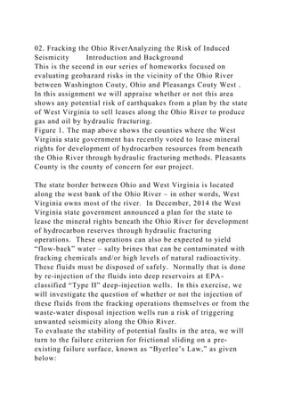Figure 1. The map above shows the counties where the West Virginia state government has recently voted to lease mineral rights for development of hydrocarbon resources from beneath the Ohio River through hydraulic fracturing methods. Pleasants County is the county of concern for our project. The state border between Ohio and West Virginia is located along the west bank of the Ohio River – in other words, West Virginia owns most of the river. In December, 2014 the West Virginia state government announced a plan for the state to lease the mineral rights beneath the Ohio River for development of hydrocarbon reserves through hydraulic fracturing operations. These operations can also be expected to yield “flow-back” water – salty brines that can be contaminated with fracking chemicals and/or high levels of natural radioactivity. These fluids must be disposed of safely. Normally that is done by re-injection of the fluids into deep reservoirs at EPA-classified “Type II” deep-injection wells. In this exercise, we will investigate the question of whether or not the injection of these fluids from the fracking operations themselves or from the waste-water disposal injection wells run a risk of triggering unwanted seismicity along the Ohio River. To evaluate the stability of potential faults in the area, we will turn to the failure criterion for frictional sliding on a pre-existing failure surface, known as “Byerlee’s Law,” as given below: For n < 200 MPa: s = 0.85n For n > 200 MPa: s = 50 MPa + 0.6n In addition, we will need information on the state of stress in the study area. We will use the closest fully determined, high quality stress estimate from the World Stress Map database, as follows: TABLE 1. Hocking County, Ohio: In situ stress measurement at a depth of 808 m determined using hydraulic fracturing techniques. azimuth of : 064° Magnitude : 24 MPa plunge of : 0° 1/2 ratio: azimuth of : 064° Magnitude of : 14 MPa plunge of : 90° azimuth of : 334° Magnitude of : 11.3 MPa plunge of : 0° 3/2 ratio: While the state of stress given above will vary somewhat from that in the Ohio River region 100 km to the east, the relative stability and uniformity of stress in the stable interior of the eastern U.S. suggests that the above stress state will provide a reasonable first approximation.Each person in your group should complete the problem set below and turn it in via Isidore. After completing this assignment, compare notes w ...

1. 02. Fracking the Ohio RiverAnalyzing the Risk of Induced
Seismicity Introduction and Background
This is the second in our series of homeworks focused on
evaluating geohazard risks in the vicinity of the Ohio River
between Washington Couty, Ohio and Pleasangs Couty West .
In this assignment we will appraise whether or not this area
shows any potential risk of earthquakes from a plan by the state
of West Virginia to sell leases along the Ohio River to produce
gas and oil by hydraulic fracturing.
Figure 1. The map above shows the counties where the West
Virginia state government has recently voted to lease mineral
rights for development of hydrocarbon resources from beneath
the Ohio River through hydraulic fracturing methods. Pleasants
County is the county of concern for our project.
The state border between Ohio and West Virginia is located
along the west bank of the Ohio River – in other words, West
Virginia owns most of the river. In December, 2014 the West
Virginia state government announced a plan for the state to
lease the mineral rights beneath the Ohio River for development
of hydrocarbon reserves through hydraulic fracturing
operations. These operations can also be expected to yield
“flow-back” water – salty brines that can be contaminated with
fracking chemicals and/or high levels of natural radioactivity.
These fluids must be disposed of safely. Normally that is done
by re-injection of the fluids into deep reservoirs at EPA-
classified “Type II” deep-injection wells. In this exercise, we
will investigate the question of whether or not the injection of
these fluids from the fracking operations themselves or from the
waste-water disposal injection wells run a risk of triggering
unwanted seismicity along the Ohio River.
To evaluate the stability of potential faults in the area, we will
turn to the failure criterion for frictional sliding on a pre-
existing failure surface, known as “Byerlee’s Law,” as given
below:

2. In addition, we will need information on the state of stress in
the study area. We will use the closest fully determined, high
quality stress estimate from the World Stress Map database, as
follows:
TABLE 1. Hocking County, Ohio: In situ stress measurement at
a depth of 808 m determined using hydraulic fracturing
techniques.
064°
24 MPa
pl
0°
064°
14 MPa
90°
334°
11.3 MPa
0°
While the state of stress given above will vary somewhat from
that in the Ohio River region 100 km to the east, the relative
stability and uniformity of stress in the stable interior of the
eastern U.S. suggests that the above stress state will provide a

3. reasonable first approximation.Each person in your group
should complete the problem set below and turn it in via
Isidore. After completing this assignment, compare notes with
your teammates and work together to complete the Seismic Risk
Analysis section of your site investigation report on Geohazard
Risks aong the Ohio River. See Team Writing Assignment 2 for
guidelines. Questions
1. To calculate stresses at various depths below, you will need
to calculate the vertical stress at the depth of interest.
a. Assuming the same state of stress as given in Hocking County
above, which of the three principle stresses is vertical? What
faulting regime would this state of stress correspond to?
(normal, reverse, or strike-slip?)
stresses at the depth of interest. Calculate these values and
enter them into the highlighted spaces in the Table 1 above.
2. The leading oil and gas “plays” in Ohio are in the Devonian
Marcellus shale and the Ordovician Utica/Pt. Pleasant shale
formations, respectively. The Ohio Geological Survey has
conveniently gathered information relating to oil and gas
production from these horizons at
http://geosurvey.ohiodnr.gov/energy-resources/marcellus-utica-
shales
In particular, you and your group should review the powerpoint
presentation on the Marcellus and Utica plays in Ohio, which is
accessible from the above web site or from the link copied
below:
http://geosurvey.ohiodnr.gov/portals/geosurvey/energy/Marcellu
s_Utica_presentation_OOGAL.pdf
For the seismic risk analysis below it is especially important for
us to know the depth to these rock layers beneath our region of
interest along the Ohio River between Washington County, OH

4. and Pleasants County, WV. We can estimate this information
from oil and gas well log data that is publically available
through the Ohio Oil and Gas Well Locator
(http://oilandgas.ohiodnr.gov/well-information/oil-gas-well-
locator). On the following page I copy the Well Summary Cards
for the Newell Run Saltwater Injection well, which lies
approximately 2.5 km north of the Ohio River. Unfortunately,
the Newell Run well does not penetrate all the way to the
Utica/Pt. Pleasant Formations. To estimate the depth to this
unit, take the depth to the contact between the Clinton and
Medina Formations shown on the Newell Run card, and estimate
the additional depth to reach the Utica-Pt. Pleasant contact from
the Protégé Energy Well. For the Marcellus, take the depth to
the base of the formation. Also, convert the depths to meters.
Table 2.
Rock Formation
Depth (ft)
Depth (m)
Marcellus shale:
Clinton/Medina Fm:
Utica/Pt. Pleasant:
3. Now that we understand the general stratigraphic and
structural setting of the Marcellus, Clinton/Medina and
Utica/Pt. Pleasant formations, we need to understand the basics

5. of hydraulic fracturing (colloquially known as “fracking”), i.e.,
what kind of fluid pressures are necessary to induce failure.
a. Using the depths given above (converted to meters), calculate
based on the stress ratios you calculated in question 1 above.
Assume that the overburden has an average density of 2400
kg/m3 In addition, calculate the hydrostatic pore fluid pressure
(Pf) at depth. Hydrostatic pore fluid pressure assumes that the
water in pore spaces forms an interconnected network to the
water table, so that pore fluid pressure can be calculated using
1000 kg/m3). The depths (h) you use should be taken from the
Table 2 above).
Table 3.
Rock Formation
Depth (m)
Pf (MPa)
Pop(MPa)
Marcellus shale:
Clinton/Medina Fm:

6. Utica/Pt. Pleasant:
construct Mohr circles on the graph paper at the end of this
assignment sheet for the estimated state of stress at the depths
of the Marcellus Shale, the Clinton/Medina formations and the
Utica/Pt. Pleasant formations. Draw your circles in different
colors for each rock type and at each level draw two Mohr
circles – one without taking pore fluid pressure into account,
and the other adjusted for hydrostatic pore fluid pressures. The
effect of pore fluid pressure is to shift the Mohr Circle to the
left by the amount of the pore fluid pressure, according to the
equation:
- Pf
c. Hydraulic fracturing involves increasing pore fluid pressure
enough to reduce effective normal stress to the point that the
effective normal stress is shifted to the left of the ordinate axis
on the Mohr diagram to intersect the tensile failure criterion.
This can happen naturally under so-called “over-pressured”
conditions, but the hydrocarbon industry has mastered how to
do this in a controlled fashion in order to increase permeability
and thus production from the ‘fracked’ rocks. In most cases,
they are seeking to take advantage of pre-existing fracture
systems known as joints. For our purposes, we will estimate the
tensile strength of both shale units at T0 = -5 MPa. Draw a red
line representing this failure criterion on your diagram, and

7. estimate the pore fluid pressure surcharge over and above the
hydrostatic pressure needed in each case to induce
hydrofracture (i.e., estimate the over-pressure Pop). Fill that
number in the far right column in Table 3 above.
4. Now, to evaluate the risk that hydrofracturie-induced
eathquakes, we need to identify potential fault planes in the
area. Historical experience suggests that there is relatively low
chance that hydrofracturing itself will directly induce felt
earthquakes unless one or more of the horizontal bores actually
intersect or closely approaches a fault. However, there is
increasing evidence that large volume injections of the
contaminated, highly saline wastewater produced by fracking
into deep disposal wells can produce earthquakes. Your written
reports should include a summary of what is known about faults
in the vicinity of the Ohio River between Washington and
Pleasants Counties. The orientations of the faults are important
in evaluating their stability as we will see below, but the
vertical and lateral extent of the faults is also important.
Simply, put, the larger the fault, the more capable it is of
producing a larger earthquake (Fig. 2). Wells and Coppersmith
(1994) formulated a scaling relationship between rupture area
and magnitude in the form of the equation: M = 0.98 log A +
4.07 (where rupture area A is in km2)
Figure 2. Graphical depiction based on global earthquake
catalogs of the logarithmic scaling relationship between rupture
area and earthquake magnitude (after Shaw et al., 2009).
a. Commonly, the length of a strike-slip fault rupture is at least
three times its depth. So if a given earthquake were to rupture a
fault that penetrated the entire sedimentary sequence from
Precambrian basement to the surface (~4 km) to the surface, it
could well form a rupture >12 km long. Assuming (as is
commonly the case) an elliptical rupture area, what would be
the area of such a rupture? Applying the equation from Wells
and Coppersmith above, what would be the approximate
magnitude of such an earthquake? (Show your work).

8. b. Could a shallow earthquake of that magnitude be of concern
if it were to occur directly beneath the Ohio River? What
would be the expected intensity of such a quake at its epicenter?
How would it compare with the largest and most severe
earthquake in Ohio history to date, the 1937 Anna earthquake?
(See
http://earthquake.usgs.gov/earthquakes/states/events/1937_03_0
9.php) Another useful comparison would be the 2011 Richmond,
Virginia earthquake (see
http://earthquake.usgs.gov/earthquakes/eqinthenews/2011/se082
311a/#details).
c. A number of resources are useful in building an inventory of
known faults in the area. In particular, you should utilize the
structure contour maps on basement (Baranoski et al., 2013), on
the top of the Trenton limestone (Patchen et al., 2006), and on
the top of the Onondaga Limestone (Wickstrom et al., 2006). In
particular, take note of the slightly different angle of the
Burning Spring Fault as represented on the maps of the
Onondaga and Trenton as contrasted with the angle represented
in the basement contour map. Presumably the orientation
represented in the Onondaga and Trenton is more pertinent here
since these are the actual horizons being fracked. Note that I
have also provided Baranoski’s structure contour map on
Precambrian basement in southeastern Ohio as a scanned
overlay in Google Earth format. In the table below, provide a
list of the faults in the area with their azimuth’s (angle
measured clockwise from North) and, where possible, the length
of each fault. For faults over 100 km long, you can simply
indicate “>100 km.” Trace each fault using the line tool in
Google Earth, and symbolize your faults as heavy red lines.

9. Note that you can save your fault map as an image file from
Google Earth using the File Save Image command. Import your
map below and use it as a figure in your written paper. Note
that some faults are named (e.g., the Rome Trough, the Burning
Spring fault, and the Cambridge structural discontinuity). To
refer to unnamed faults, assign them letters in your Google
Earth map and refer to them by the corresponding letter in the
table below:
Fault Name
Azimuth
Fault Length
Rome Trough:
Burning Spring:
Cambridge Discontinuity
Unnamed Fault A
Unnamed Fault B
d. Once you have the fault azimuths recorded, you can now

10. of maximum principle stress. Fill in the columns in the table
above and mark and label the corresponding point on each of
your Mohr Circles at the end of the hand-out. We will again
turn to Byerlee’s Law to evaluate the stability or instability of
the faults you identified. Plot Byerlee’s Law on your Mohr
diagram and use it to evaluate the stability or instability of the
faults. In the space below list each fault and identify whether,
given our assumptions above, it would be stable, unstable or
near-critical (a) under hydrostatic stress conditions, and (b)
during fracking.
5. Finally, having conducted the above mechanical analysis, we
can also look at whether there is any evidence in the area that
past injection activities have triggered induced seismicity.
Although there has not yet been widespread fracking activity in
Washington County, there are a number of Class II deep
injection wells and also some recent small earthquakes in the
area. The Google Earth data file I have provided already
includes the locations of the two largest of the recent
earthquakes in the county. To locate the other epicenters go to
the OhioSeis network homepage at:
http://geosurvey.ohiodnr.gov/earthquakes-ohioseis/ohioseis-
home and open the “Recent Events” list. Scroll down the list
looking for events located in Washington County. When you
find one, copy the latitude and longitude and paste it into the
search window of Google Earth. For example, Lat. 39.4096o
North, Long -81.3940o West would be pasted in the form
39.4096, -81.3940 (by convention West longitudes are
negative). If you open the Properties for this point and go to
the “Style, Color” tab you can choose from a menu of symbols,
including an earthquake symbol. You can also copy and paste
the description of the earthquake from Ohioseis, and if you wish
you may insert a hyperlink that will open the Ohioseis web page

11. in Google Earth. There are also several injection wells in
Washington County. The locations of these can be found in the
Ohio Oil and Gas well locator web page at:
https://gis.ohiodnr.gov/website/dog/oilgasviewer/. The state
makes this information open to the public utilizing a leading
GIS software package, ARCGIS Online; ARCGIS is the same
system taught in UD’s graduate certificate program in
Geographic Information Systems. After opening the viewer
zoom into Washington County – are you surprised at how many
holes have been drilled in this area? I was! Though fracking in
the Utica and Marcellus is new, traditional oil production from
units such as the Trenton and the Clinton/Medina has a long
history in Ohio. Here we are only interested in the injection
wells as those are the ones that have occasionally been
associated with induced seismicity. Once again, I have already
located the first two wells for you. All petroleum-related wells
(including Class II injection wells) are assigned unique
identifying numbers known as “API numbers” by the American
Petroleum Institute. You can locate the wells of interest by
using the search tool to locate them using their API numbers, as
listed below:
API Number
Well name
DTD
Completion Formation
Injection Formation
Injection Pressure
34167293950000
Ohio Oil Gathering Corp. II, SWIW (Salt Water Injection Well)
#6
34167295770000
Helen F. Hall, SWIW #7

12. 34167296580000
Long Run Disposal Well, SWIW #8
34167296850000
Newell Run, SWIW #10 (already located on map for you)
7332 ft 2235 m
Queenston shale
Clinton
Medina
1950 psi 13.4 MPa
34167296180000
Greenwood Unit, SWIW #15
7451 ft 2271 m
Queenston shale
Clinton
Medina
1690 psi 11.7 MPa
34167297190000
Sawmill Run Disposal Well, SWIW #16
As you search for and locate each well above, you can use the
“Information” tool to click on the well and open an information
pop-up that includes a hyperlink to a Well Summary Report.
From the Well Summary Report you can also link to the well
card (which generally includes a stratigraphic log) and various

13. other documents relating to the well, typically including the
well permit. In the case of an injection well, there should be at
least one permit that specifies the maximum allowable surface
injection pressure (in psi) that the well is licensed to pump at.
In order to consider how this pressure would affect our Mohr
circles, convert it to MPa (this is easily done with online
conversion utilities). For each well, record the DrilledTotal
Depth (DTD), what formation the well was completed in, and
what interval the injection is occurring in, and the maximum
licensed surface injection pressure in the table above.
Once you have located the wells and the earthquake epicenters
study your map to determine whether any of the recent
earthquakes occurred in close proximity to an injection well.
a. Considering both the epicentral location and the depth, which
earthquake was located closest to an injection well, and how
close was it? (Use the measurement tool in Google Earth)
b. Construct a Mohr circle for the depth of the injection well
and adjust it for hydrostatic pressure plus the maximum allowed
injection pressure for the pertinent well from the table above. In
this case we do not know the fault orientation, but does it seem
credible that the well could have induced the earthquake?
c. How far is the well in question from the nearest known fault?
How far is it from the Willow Island dam site or the McElroy’s
Run earthen embankment dam? Could a large earthquake on the
fault put the dam at risk/?
d. All things considered, is there einough risk of significant
induced seisimicity in the area to merit further investigation of
this potential hazard?
ReferencesBaranoski, Mark T., 2013, Structure contour map on

14. the Precambrian unconformity surface in Ohio and related
basement features (vers 2.0), Ohio Dept. Natural Resources,
Division of the Geological Survey, Map PG-23, Scale
1:500,000, 17 p. text.Heidbach, O., Tingay, M., Barth, A.,
Reinecker, J., Kurfeß, D. and Müller, B.,
The World Stress Map database release 2008
doi:10.1594/GFZ.WSM.Rel2008, 2008.
Ohio Department of Natural Resources, March, 2012,
Preliminary Report on Northstar 1 Class II Injection Well and
the Seismic Events in the Youngstown Ohio Area.
Patchen, D.G., Hickman, J.B., Harris, D.C., Drahovzal, J.A.,
Lake, P.D., Smith, L.B., Nyahay, Richard, Schulze, Rose, Riley,
R.A., Baranoski, M.T., Wickstrom, L.H., Laughrey, C.D.,
Kostelnik, Jaime, Harper, J.A., Avary, K.L., Bocan, John, Hohn,
M.E., and McDowell, Ronald, 2006, A geologic play book for
Trenton-Black River Appalachian Basin exploration:
Morgantown, W. Va., U.S. Department of Energy Report, DOE
Award Number DE-FC26-03NT41856, 601p., accessible at
<http://www.wvgs.wvnet.edu/www/tbr/project_reports.asp>.
Shaw, B. E. (2009). Constant stress drop from small to great
earthquakes in magnitude–area scaling, Bull. Seismol. Soc. Am.
99, 871–875, doi: 10.1785/0120080006.
Wells, D. L., and K. J. Coppersmith (1994). New empirical
relationships among magnitude, rupture length, rupture width,
rupture area and surface displacement, Bull. Seismol. Soc. Am.
84, 974–1002.
Wickstrom, L.H., Perry, C.J., Riley, R.A., and others, 2006,
Marcellus & Utica Shale: Geology, History and Oil & Gas
Potential in Ohio. Map modified by Powers, D.M. and Martin,
D.R.
Figure 3. Map of known bedrock fault systems in Ohio (Ohio
Dept. Nat. Res. Div. of Geol. Surv.)
Figure 4. Map of historic earthquake epicenters in Ohio scaled

15. by magnitude.
Figure 5. Locations of deep injection waste disposal wells in
Ohio.
GEO301: Structural Geology
Name:_____________________________________

16. Marcellus Shale

52. Utica/Pt. Pleasants Formations

89. Clinton/Medina Sandstone