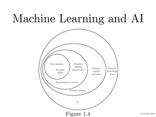
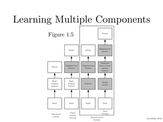
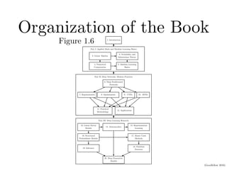
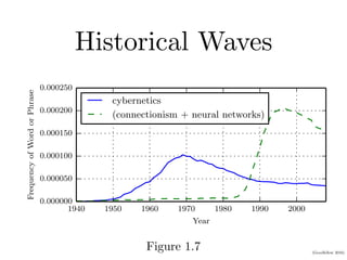
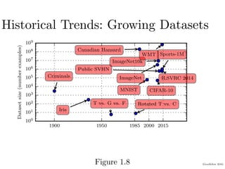
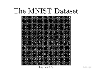
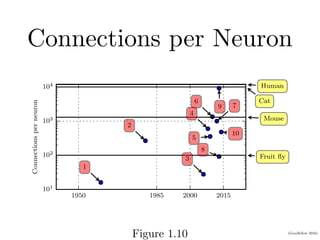
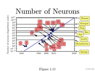
Introduction
Lecture slides for Chapter 1 of Deep Learning
www.deeplearningbook.org
Ian Goodfellow
2016-09-26
(Goodfellow 2016)
Representations Matter
APTER 1. INTRODUCTION
x
y
Cartesian coordinates
r
θ
Polar coordinates
ure 1.1: Example of different representations: suppose we want to separate
Figure 1.1
(Goodfellow 2016)
Depth: Repeated Composition
CHAPTER 1. INTRODUCTION
Visible layer
(input pixels)
1st hidden layer
(edges)
2nd hidden layer
(corners and
contours)
3rd hidden layer
(object parts)
CAR PERSON ANIMAL
Output
(object identity)
Figure 1.2: Illustration of a deep learning model. It is difficult for a computer to understand
the meaning of raw sensory input data, such as this image represented as a collection
Figure 1.2
(Goodfellow 2016)
Computational Graphs
CHAPTER 1. INTRODUCTION
x1
x1
w1
w1
⇥
x2
x2
w2
w2
⇥
+
Element
Set
+
⇥
x
x
w
w
Element
Set
Logistic
Regression
Logistic
Regression
Figure 1.3: Illustration of computational graphs mapping an input to an output where
each node performs an operation. Depth is the length of the longest path from input to
Figure 1.3
(Goodfellow 2016)
Machine Learning and AI
AI
Machine learning
Representation learning
Deep learning
Example:
Knowledge
bases
Example:
Logistic
regression
Example:
Shallow
autoencoders
Example:
MLPs
Figure 1.4: A Venn diagram showing how deep learning is a kind of representation learning,
Figure 1.4
(Goodfellow 2016)
Learning Multiple Components
CHAPTER 1. INTRODUCTION
Input
Hand-
designed
program
Output
Input
Hand-
designed
features
Mapping from
features
Output
Input
Features
Mapping from
features
Output
Input
Simple
features
Mapping from
features
Output
Additional
layers of more
abstract
features
Rule-based
systems
Classic
machine
learning Representation
learning
Deep
learning
Figure 1.5
(Goodfellow 2016)
Organization of the Book
CHAPTER 1. INTRODUCTION
1. Introduction
Part I: Applied Math and Machine Learning Basics
2. Linear Algebra
3. Probability and
Information Theory
4. Numerical
Computation
5. Machine Learning
Basics
Part II: Deep Networks: Modern Practices
6. Deep Feedforward
Networks
7. Regularization 8. Optimization 9. CNNs 10. RNNs
11. Practical
Methodology
12. Applications
Part III: Deep Learning Research
13. Linear Factor
Models
14. Autoencoders
15. Representation
Learning
16. Structured
Probabilistic Models
17. Monte Carlo
Methods
18. Partition
Function
19. Inference
20. Deep Generative
Models
Figure 1.6: The high-level organization of the book. An arrow from one chapter to another
Figure 1.6
(Goodfellow 2016)
Historical Waves
1940 1950 1960 1970 1980 1990 2000
Year
0.000000
0.000050
0.000100
0.000150
0.000200
0.000250
Frequency
of
Word
or
Phrase
cybernetics
(connectionism + neural networks)
ure 1.7: The figure shows two of the three historical waves of artificial neural
Figure 1.7
(Goodfellow 2016)
Historical Trends: Growing Datasets
1900 1950 1985 2000 2015
Year
100
101
102
103
104
105
106
107
108
109
Dataset
size
(number
examples)
Iris
MNIST
Public SVHN
ImageNet
CIFAR-10
ImageNet10k
ILSVRC 2014
Sports-1M
Rotated T vs. C
T vs. G vs. F
Criminals
Canadian Hansard
WMT
ure 1.8: Dataset sizes have increased greatly over time. In the early 1900s, statistician
died datasets using hundreds or thousands of manually compiled measurements (Garson
0; Gosset, 1908; Anderson, 1935; Fisher, 1936). In the 1950s through 1980s, the pioneer
iologically inspired machine learning often worked with small, synthetic datasets, suc
Figure 1.8
(Goodfellow 2016)
The MNIST Dataset
CHAPTER 1. INTRODUCTION
Figure 1.9: Example inputs from the MNIST dataset. The “NIST” stands for National
Figure 1.9
(Goodfellow 2016)
Connections per Neuron
1950 1985 2000 2015
Year
101
102
103
104
Connections
per
neuron
1
2
3
4
5
6
7
8
9
10
Fruit fly
Mouse
Cat
Human
Figure 1.10: Initially, the number of connections between neurons in artificial neura
networks was limited by hardware capabilities. Today, the number of connections between
neurons is mostly a design consideration. Some artificial neural networks have nearly a
Figure 1.10
(Goodfellow 2016)
Number of Neurons
1950 1985 2000 2015 2056
Year
10 2
10 1
100
101
102
103
104
105
106
107
108
109
1010
1011
Number
of
neurons
(logarithmic
scale)
1 2
3
4
5
6
7
8
9
10
11
12
13
14
15
16
17
18
19
20
Sponge
Roundworm
Leech
Ant
Bee
Frog
Octopus
Human
ure 1.11: Since the introduction of hidden units, artificial neural networks have doub
ize roughly every 2.4 years. Biological neural network sizes from Wikipedia (2015
1. Perceptron (Rosenblatt, 1958, 1962) Figure 1.11
(Goodfellow 2016)
Solving Object Recognition
2010 2011 2012 2013 2014 2015
Year
0.00
0.05
0.10
0.15
0.20
0.25
0.30
ILSVRC
classification
error
rate
gure 1.12: Since deep networks reached the scale necessary to compete in the Ima
arge Scale Visual Recognition Challenge, they have consistently won the compe
ery year, and yielded lower and lower error rates each time. Data from Russak
Figure 1.12

01_introduccion a redes neuronales artificiales.pdf

  • 1.
    Introduction Lecture slides forChapter 1 of Deep Learning www.deeplearningbook.org Ian Goodfellow 2016-09-26
  • 2.
    (Goodfellow 2016) Representations Matter APTER1. INTRODUCTION x y Cartesian coordinates r θ Polar coordinates ure 1.1: Example of different representations: suppose we want to separate Figure 1.1
  • 3.
    (Goodfellow 2016) Depth: RepeatedComposition CHAPTER 1. INTRODUCTION Visible layer (input pixels) 1st hidden layer (edges) 2nd hidden layer (corners and contours) 3rd hidden layer (object parts) CAR PERSON ANIMAL Output (object identity) Figure 1.2: Illustration of a deep learning model. It is difficult for a computer to understand the meaning of raw sensory input data, such as this image represented as a collection Figure 1.2
  • 4.
    (Goodfellow 2016) Computational Graphs CHAPTER1. INTRODUCTION x1 x1 w1 w1 ⇥ x2 x2 w2 w2 ⇥ + Element Set + ⇥ x x w w Element Set Logistic Regression Logistic Regression Figure 1.3: Illustration of computational graphs mapping an input to an output where each node performs an operation. Depth is the length of the longest path from input to Figure 1.3
  • 5.
    (Goodfellow 2016) Machine Learningand AI AI Machine learning Representation learning Deep learning Example: Knowledge bases Example: Logistic regression Example: Shallow autoencoders Example: MLPs Figure 1.4: A Venn diagram showing how deep learning is a kind of representation learning, Figure 1.4
  • 6.
    (Goodfellow 2016) Learning MultipleComponents CHAPTER 1. INTRODUCTION Input Hand- designed program Output Input Hand- designed features Mapping from features Output Input Features Mapping from features Output Input Simple features Mapping from features Output Additional layers of more abstract features Rule-based systems Classic machine learning Representation learning Deep learning Figure 1.5
  • 7.
    (Goodfellow 2016) Organization ofthe Book CHAPTER 1. INTRODUCTION 1. Introduction Part I: Applied Math and Machine Learning Basics 2. Linear Algebra 3. Probability and Information Theory 4. Numerical Computation 5. Machine Learning Basics Part II: Deep Networks: Modern Practices 6. Deep Feedforward Networks 7. Regularization 8. Optimization 9. CNNs 10. RNNs 11. Practical Methodology 12. Applications Part III: Deep Learning Research 13. Linear Factor Models 14. Autoencoders 15. Representation Learning 16. Structured Probabilistic Models 17. Monte Carlo Methods 18. Partition Function 19. Inference 20. Deep Generative Models Figure 1.6: The high-level organization of the book. An arrow from one chapter to another Figure 1.6
  • 8.
    (Goodfellow 2016) Historical Waves 19401950 1960 1970 1980 1990 2000 Year 0.000000 0.000050 0.000100 0.000150 0.000200 0.000250 Frequency of Word or Phrase cybernetics (connectionism + neural networks) ure 1.7: The figure shows two of the three historical waves of artificial neural Figure 1.7
  • 9.
    (Goodfellow 2016) Historical Trends:Growing Datasets 1900 1950 1985 2000 2015 Year 100 101 102 103 104 105 106 107 108 109 Dataset size (number examples) Iris MNIST Public SVHN ImageNet CIFAR-10 ImageNet10k ILSVRC 2014 Sports-1M Rotated T vs. C T vs. G vs. F Criminals Canadian Hansard WMT ure 1.8: Dataset sizes have increased greatly over time. In the early 1900s, statistician died datasets using hundreds or thousands of manually compiled measurements (Garson 0; Gosset, 1908; Anderson, 1935; Fisher, 1936). In the 1950s through 1980s, the pioneer iologically inspired machine learning often worked with small, synthetic datasets, suc Figure 1.8
  • 10.
    (Goodfellow 2016) The MNISTDataset CHAPTER 1. INTRODUCTION Figure 1.9: Example inputs from the MNIST dataset. The “NIST” stands for National Figure 1.9
  • 11.
    (Goodfellow 2016) Connections perNeuron 1950 1985 2000 2015 Year 101 102 103 104 Connections per neuron 1 2 3 4 5 6 7 8 9 10 Fruit fly Mouse Cat Human Figure 1.10: Initially, the number of connections between neurons in artificial neura networks was limited by hardware capabilities. Today, the number of connections between neurons is mostly a design consideration. Some artificial neural networks have nearly a Figure 1.10
  • 12.
    (Goodfellow 2016) Number ofNeurons 1950 1985 2000 2015 2056 Year 10 2 10 1 100 101 102 103 104 105 106 107 108 109 1010 1011 Number of neurons (logarithmic scale) 1 2 3 4 5 6 7 8 9 10 11 12 13 14 15 16 17 18 19 20 Sponge Roundworm Leech Ant Bee Frog Octopus Human ure 1.11: Since the introduction of hidden units, artificial neural networks have doub ize roughly every 2.4 years. Biological neural network sizes from Wikipedia (2015 1. Perceptron (Rosenblatt, 1958, 1962) Figure 1.11
  • 13.
    (Goodfellow 2016) Solving ObjectRecognition 2010 2011 2012 2013 2014 2015 Year 0.00 0.05 0.10 0.15 0.20 0.25 0.30 ILSVRC classification error rate gure 1.12: Since deep networks reached the scale necessary to compete in the Ima arge Scale Visual Recognition Challenge, they have consistently won the compe ery year, and yielded lower and lower error rates each time. Data from Russak Figure 1.12