Department of Economics, University at Buffalo Winston Chang.docx

Department of Economics, University at Buffalo Winston Chang
For use by students of my course only. Further distribution is
prohibited.1
Simple Pure Exchange Models
1 Introduction
The price of a good or service observed in a national market,
without foreign trade, is determined
by demand and supply in that nation. On the supply side,
nations generally have different natural
endowments, different factors of production, and different
technologies relevant to the production
of goods and services. These differences result in variations in
production costs. On the demand
side, people have different incomes and tastes, which generate
unique patterns of demand among
nations. Thus, the autarkic prices observed among nations tend
to be different. Once foreign
trade is opened up, goods and services move between nations.
Some questions that come to mind
when considering foreign trade are: Which country exports
which good? What role do autarkic

prices play in determining the direction of trade? What are the
equilibrium terms of trade? Are
there gains from trade? These are some of the basic questions to
be answered in the study of
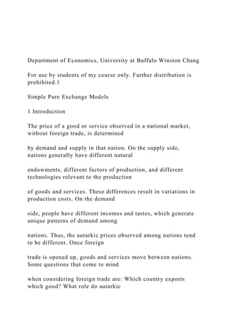
international economics.
In this chapter, we will consider some simple exchange models
in order to illustrate the deter-
minants of trade. It will be shown that it is the difference in
relative autarkic prices, not money
prices, that causes trade to take place. We will also examine the
determination of the equilibrium
terms of trade and gains from trade with the help of a simple
exchange model, while keeping the
supply of goods fixed.
2 The Determinants of Barter Trades
To illustrate the basic determinants of trade, we consider a very
simple pure exchange model in
which there are two countries, called home (H) and foreign (F),
and two goods, good 1 (G1)
1Copyright c
2009 by Winston Chang. All rights reserved.
1

and good 2 (G2). Goods are already produced so there are no
new production activities in either
country. Before trade is opened up, each good has an autarkic
price in each country. Let the home
country’s variables be represented without an asterisk and
foreign variables with an asterisk. Let
pj be the money price of goodj in H (j = 1;2), measured, say, in
U.S. dollars andp
�
j be the money
price of goodj in F (j = 1;2), measured in British pounds. These
are the money (nominal) prices
observed in the autarkic (no foreign trade) equilibrium. Assume
that there are no impediments to
trade; namely, there are no transport costs or other trading
costs. The markets are competitive,
and the buyers and sellers all face the same prices. How is the
trade pattern determined? Is it
determined by these nominal prices?
To answer both questions, we first consider a barter exchange
economy in which one good is
directly exchanged for the other. Since there are no trading
costs, if the barter exchange ratios

between the two goods in the two countries are different,
gainful arbitrage activities will take place
and trade will occur. A barter exchange ratio is nothing but the
nominalprice ratio . Let p =
p1=p2 which is called "the relative price of G1 (in terms of
G2)" in H. It measuresp units of G2
that are exchanged for one unit of G1. For example, ifp1 = 10
andp2 = 5; thenp = 2, which
means one unit of G1 can be exchanged for two units of G2.
Formally,p1=p2 has the dimension of�
$10
1G1
�
=
�
$5
1G2
�
= 2G2/1G1. The $ element is canceled out in the ratiop1=p2:
Similarly, the relative
price of G2 (in terms of G1) in H is1=p = p2=p1: The foreign
autarkic relative price of G1 in terms
of G2 isp� = p�1=p
�
2:
The following proposition shows that the determinants of trade
are not the nominal autarkic

prices but the relative autarkic prices.
Proposition 1 Barter trade between a pair of goods can gainfully
take place if theautarkic rela-
tive pricesbetween the pair of goods in the two countries are
different. A country will export the
good whose relative autarkic price is cheaper than the other’s,
and both countries can gain from
the trade.
2
Consider the following autarkic price matrix:
2
64 p1 p�1
p2 p
�
2
3
75 =
2
64 1 40
2 10
3
75 : (1)

From this matrix, we know that one unit of G1 in H can be
exchanged for 0.5 units of G2 (p =
1=2 = 0:5); but in the foreign country, one unit of G1 can be
exchanged for four units of G2
(p� = 40=10 = 4): So if a merchant ships one unit of G1 from H
to F, he can exchange that unit for
four units of G2 in F, compared with only 0.5 units of G2 in H.
He will therefore have a gain of 3.5
units of G2. If this gain is more than enough to pay for the
transportation and other transactions
costs, he will gain from the trade and export G1.
Now think of F. Under autarky, a unit of G2 can be exchanged
forp�2=p
�
1 � 1=p� = 10=40 =
0:25 units of G1: If a merchant ships one unit of G2 from F to
H, he can exchange that unit for
p2=p1 = 2=1 = 2 units of G1. He will gain 1.75 units of G1.
Thus, F will export G2. Unequal
relative prices create the opportunity for profitable arbitrage,
and since both countries gain from
this transaction, trade emerges voluntarily.
The above example illustratesa fundamental principle: if, under
autarky,p1=p2 < p

�
1=p
�
2; then
H will export G1, and F will export G2. It is easy to verify that
ifp1=p2 > p
�
1=p
�
2; then the opposite
trade pattern occurs. Thus, wheneverp1=p2 6= p�1=p�2; trade
will take place. Furthermore, both
countries gain from trade.
Note that the relative prices are independent of currency units
used in each country. If H is the
U.S., F is the U.K., and$1 = $1; then the U.K.’s autarkic money
prices in terms of dollars are both
higher than those in the U.S. If trade was thought to be
determined by comparing the money prices,
then the U.K. would not have been able to export any good. It is
theautarkic relative prices that
matter in the determination of the pattern of barter trade, not
thenominal money prices. Since
the currency exchange rate has no bearing on relative prices, it
is not a factor in determining the

pattern of trade in the barter exchange model.
3
3 A Simple Model of Trade with Fixed Initial Endowments
The basis for barter trade is the difference in autarkic relative
prices. What causes the autarkic
relative prices to be different between countries? Some of the
factors that come to mind are differ-
ent tastes, different endowments, and different costs of
production. Identical tastes with different
endowments among traders can cause trade. Similarly, identical
endowments with different tastes
can also cause trade. In this section, we study a simple pure
exchange economy that allows for
different tastes and different fixed endowments. There are no
production activities in this model.
Goods are already produced and are in fixed supply. LetSj
andDj be the supply and demand
(consumption) of Gj in H, andS�j andD
�
j be their counterparts in F(j = 1;2). Assume H exports
G1 and imports G2. LetX andM be the exports and imports of H
andX� andM� be the foreign

counterparts:
X � S1 �D1; M � D2 �S2
X� � S�2 �D
�
2; M
� � D�1 �S
�
1 (2)
H’s national expenditure under autarky isp1D1 +p2D2, and its
GDP isp1S1 +p2S2, which is also
its national income. By the national income identity,p1D1 +
p2D2 = p1S1 + p2S2: Under free
trade, domestic prices are equal to foreign prices (assuming that
the same currency units are used
or that the units of currencies are redefined so that the exchange
rate is one). The home country’s
budget constraint is
p1D1 +p2D2 = p1S1 +p2S2; (3)
which shows that a country’s national expenditure is equal to its
national income.2 Rearranging
terms, we havep1 (S1 �D1) = p2 (D2 �S2) ; which yields the
following balance-of-trade equi-
librium condition under free trade (pj = p

�
j):
p�1X = p
�
2M , p
�X = M: (4)
2Note that the prices and the demand and supply configurations
will be different between autarky and free trade
in both countries. For ease of notation, we continue using the
same notations in both situations.
4
This condition shows that the home country’s total value of
exports is equal to the total value of
imports, evaluated at world prices.
Analogously, F’s budget constraint is
p�1D
�
1 +p
�
2D
�
2 = p
�

1S
�
1 +p
�
2S
�
2; (5)
which implies
p�1M
� = p�2X
� , p�M� = X�: (6)
Equilibrium in the world markets requires that total world
demand be equal to total world
supply for each good:
D1 +D
�
1 = S1 +S
�
1; (7)
D2 +D
�
2 = S2 +S
�
2; (8)

which are equivalent to
X = M�; (9)
X� = M: (10)
The two market-clearing conditions in (7) and (8) are not
independent. By summing the two
countries’ budget constraints in (3) and (5) and noting that
under free trade,pj = p
�
j; we obtain
p�1 (D1 +D
�
1 �S1 �S
�
1)+p
�
2 (D2 +D
�
2 �S2 �S
�
2) = 0: (11)
Given thatp�1 > 0 andp
�
2 > 0; if one market is in equilibrium (either (7) or (8) holds),
the other

market must also be in equilibrium. This isWalras’ Law . In
mathematical terms, the two market-
clearing conditions are not independent of each other. Eq. (11)
can be alternatively expressed
5
as
p�1 (M
� �X)+p�2 (M �X
�) = 0: (12)
M� �X is the world excess demand for G1 andM �X� the
world excess demand for G2. Thus,
Walras’ Law says thatthe sum of the values of world excess
demands in both markets is zero.
It follows thatM� = X if and only if M = X�:
Walras’ Law as expressed in (11) can be readily generalized to
then-good case. Let the world
excess demand for Gj beEj �
�
Dj +D
�
j
�

�
�
Sj +S
�
j
�
: Then, Walras’ Law in then-good case is
nX
j=1
p�jEj = 0: (13)
This indicates thatthe sum of the values of world excess
demands over all markets must be zero.If
anyn�1 markets are in equilibrium, the remaining one must also
be in equilibrium.
3.1 The Gains from Trade in a Pure Exchange World Economy
To analyze the existence of gains from trade, consider the
simple two-country, two-good model
with fixed endowments. PointE in Fig. 1 is H’s endowment
point with(S1;S2) measured from
the origin0. It is also F’s endowment point with(S�1;S
�
2) measured from the origin0
�. The size
of the box is determined by the fixed world supplies of both

goods. The horizontal axis measures
the demands for G1 in both countries, and the vertical axis
measures demand for G2. Assume that
each country has an aggregate utility function that only depends
on the bundle of consumption.
The autarkic utility levels are illustrated by the indifference
curvesU0 = U (D1;D2) = U (S1;S2)
andU�0 = U
� (D�1;D
�
2) = U
� (S�1;S
�
2) for H and F, respectively. For H, the consumption set
bounded below by theU0 curve is preferred to autarky, and for
F, the consumption set bounded
below by theU�0 curve in reference to its origin is also
preferred to autarky. Thus, the mutually
compatible preferred region is in the lensEABA�. If the two
countries can exchange goods so
that the final consumption point lies in the lens, then both are
better off with trade. This lens is
called the bargaining set. For H, the highestU achievable
subject to the bargaining set is pointA;

6
and for F, it isA�. The line0A�A0� is the locus of the tangent
points of the two indifference maps.
This locus is calledthe contract curve (and also called the
conflict curve). It has the property that
any move from a point on the contract curve will necessarily
lower at least one party’s utility. The
contract curve is the set of Pareto efficient allocations. A point
off the contract curve such asG
in Fig. 1 is not Pareto efficient since a new allocation away
fromG toward the contract curve can
improve at least one party’s utility without having to reduce the
other’s. It follows that an efficient
outcome with the initial bargaining point atE must settle at a
point in the segmentAA� of the
contract curve. This segment is calledthe "core" of the
economy. If the reallocation is achieved
through the bargaining process in the two party world, the final
outcome is in the core. The exact
outcome depends on relative bargaining skills and other factors
in the bargaining process.
Figure 1:
The box diagram in a simple exchange model

*
2S2S
*A
*0
*
0U
*
1U
1U
0U
B
A
G
0
1S 1
D
E
2D *1S*
1D
C
*
2D

Consider now the case in which each country has many traders
and therefore the economy
is a competitive one—each trader is a price taker and the market
prices are influenced by the
market excess demand or supply of the goods. A representative
trader facing market prices tries
to maximize their utility subject to the budget constraint. If all
traders in a country are identical,
7
then the home country’s traders will chooseD1 andD2 to
maximizeU (D1;D2) subject to (3), or
equivalently
pD1 +D2 = pS1 +S2: (14)
Each solvedDj is a function ofp andpS1 + S2, which is the
national income in terms of G2.
3
With S1 andS2 fixed in the present model, the national income
is also a function ofp, which is the
terms of trade. Thus,Dj = Dj (p) : Similarly, for F,D
�
j = D
�
j (p

�) :
Under free trade,p = p�: The equilibriump� is determined by
the market clearing conditions.4
As already discussed, Walras’ Law implies that only one of the
market equilibrium conditions in
(7) and (8) is needed for this purpose. Take, for example, the
G1 market clearing condition (7):
D1 (p)+D
�
1 (p
�) = S1 +S
�
1: (15)
This equation can be used to solve for the equilibrium terms of
tradep�(= p): Clearly, the equilib-
rium p� is determined byS1 + S
�
1 and the underlying preferences of both countries. Fig. 2 is the
graphical representation of (15).
Alternatively, one can use the export and import functions to
solve for the equilibriump�: From
(15), we can rewrite (9) asX (p) = M� (p�) ; which can be
solved for the same solution set. Fig. 3
shows this alternative way of determining the equilibrium terms

of trade.
3To solve this problem, set up the Lagrangian
functionL(D1;D2;�) = U (D1;D2) +
�(pS1 +S2 �pD1 �D2) ; where � is the Lagrange multiplier.
By embedding the constraint into the La-
grangian function and introducing the new variable�, the
original constrained maximization problem is equivalent
to maximizing the unconstrainedL function with respect to the
three variables,D1; D2 and �: The first-order
conditions are:@[email protected] = U1 � �p = 0;
@[email protected] = U2 � � = 0
[email protected][email protected]� = pS1 + S2 � pD1 � D2 =
0;
whereUj � @[email protected]: These three conditions are used
to solve for the three variables. Note that from the first two
conditions, we haveU1=U2 = p; namely, the marginal utility
ratio is the price ratio at the optimum. Let the utility
attained at the optimum be�U: From the indifference curveU
(D1;D2) = �U; we haveU1dD1 + U2dD2 = 0; which
implies that the marginal rate of substitution
(MRS)�dD2=dD1jU=�U is equal toU1=U2; and hence is equal
top:
4In the pure exchange model with no specification of the money
markets, the nominal money prices(p�1;p
�
2) are
indeterminate. This is seen by noting that if(p�1;p
�
2) is a solution, then(�p
�
1;�p

�
2) is also a solution for any� > 0:
By changing all money prices by the same proportion, the
budget constraints are unaffected, and the money income is
also changed by the same proportion. Thus, the chosen demands
will remain unchanged and the chosen trade volumes
will also be unchanged; here only the relative price matters.
8
Figure 2:
The determination of the equilibrium terms of trade
p=p*
*
1 1S S+
( ) ( )*1 1 *p DD p+
0
* *
1 1 1 1, SD D S+ +
p, p*
3.2 The Offer Curves
Consider Fig. 4, in whichE is the endowment point of the home
country. The budget constraint
in (3) are lines that go through pointE under different prices.

Ifp� = a; the highest utility
attainable under the budget lineEK is Ua with the preferred
consumption point atK: Similarly,
at p� = b; the preferred consumption point isN: The collection
of all the preferred consumption
points for different values ofp� is the curveEKN: This curve,
viewed from the origin0; is a price
consumption curve; if viewed from the new originE; it is the
offer curve. Atp� = a; H will offer
EY of G1 for YK of G2. At p� = b; H will offer EZ of G1 for
ZN of G2. The offer curve thus
portrays the utility-maximizing bundle of desired trade for
various values ofp�: If the price line is
sufficiently flat (the relative price of G1 is sufficiently low),
the desired trading point moves to the
south-east region ofE: In this case, the trade pattern is
reversed—H will want to export G2 and
import G1. Depending upon the indifference map, the offer
curve can have quite different shapes.
9
Figure 3:
p=p*

( )X p
( )* *M p
0
*,X M
p, p*
Fig. 5 plots the offer curve in the(X;M) axes. It is the mirror-
image of Fig. 4 withE as the new
origin. This curve shows thereciprocal demands schedule, which
demonstrates that a nation’s
exports are for the purpose of obtaining imports. There are no
free meals on earth. As the terms
of tradep� moves froma to b; the optimal trading point moves
fromK to N: LinesEa andEb are
generated by the balance-of-trade equilibrium condition given
in (4). An increase inp�, which is
the same as an increase inM=X, gives the home country
improved terms of trade, in which a unit
of exports can be exchanged for more units of imports.
3.3 Determination and Stability of a Trading Equilibrium
The foreign country’s offer curve is the mirror image of the
home’s, with the horizontal axisM�(in
G1) and the vertical axisX� (in G2). By superimposing the

home and foreign offer curves in one
graph, we obtain Fig. 6.
Equilibrium occurs at the intersection pointT of the two offer
curves0O and 0O�: At T;
X = M�, andM = X�, both markets are cleared. Desired exports
of one country are matched by
10
Figure 4:
Derivation of the offer curve
the desired imports of the other. Trade can therefore take place
at theequilibrium terms of trade
p�: Clearly, at the trading pointT; both countries’ balances of
trade are in equilibrium:p�X =
M = X� = p�M�:
The attainment of the equilibriump� in a competitive economy
should be addressed further.
Suppose that temporarily the price line is0a as shown in Fig. 6.
H’s chosen trading point isK and
F’s isJ: In this case, we haveM� > X andM < X�: G1 has
excess demand in the world market
and G2 excess supply. It is reasonable to hypothesize that if a
good is in excess demand, its price

will rise, and if in excess supply, its price will fall. If trade can
only take place given a contract that
matches the desired trading volumes of both traders, then at the
price line0a, the desired trading
volumes wouldn’t match, and therefore, the competitive market
force will push upp�1 and push
downp�2: Thus, the price ratiop
� (� p�1=p�2) will go up. This process will continue as long
as the
11
Figure 5:
The offer curve
ZY
N
X
M
E
a
K
O

b
markets are not cleared. Eventually, the equilibrium price
line0T is reached, and the equilibrium
terms of tradep�are established.
From the offer curve analysis, one can easily verify Walras’
Law. At the price line0a; the price
ratio isp�a1 =p
�a
2 : G1 has a world excess demand in the amount ofM
��X, and G2 has a world excess
supply ofX� �M: The slope of the0a line isp�a1 =p�a2 ,
which is equal to(X� �M)=(M� �X) :
Thus,p�a1 (M
� �X) = p�a2 (X� �M) ; or equivalently,p�a1 (M� �X) +
p�a2 (M �X�) = 0; is
Walras’ Law as already shown in (12).
3.4 The Possibility of Multiple Equilibria
As previously mentioned, since the shape of an offer curve
depends on the indifference map and
the initial endowments, it can exhibit strange shapes. Fig. 7
illustrates a case of multiple equilibria.
12

Figure 6:
Trading equilibrium
J
V
W
a
ZY
T
X, M*
M, X*
0
K
O
p*
O*
It has three equilibrium terms of trade. It can be verified that if
the price line is in the conep�0p�00
or below it, the price ratio will converge towardp�0. But if it is
in the conep�00p�000 or above it,

the price ratio will converge towardp�000. Thus,p�0 andp�000
are stable butp�00 is unstable. A slight
disturbance of the price away fromp�00 will accelerate the
price divergence toward eitherp�0 or p�000:
4 Example: Price Formation in P.O.W. Camps
R. A. Radford was an Allied prisoner of war in Italian and
German prison camps during WWII. In
Radford(1945), he documents how markets developed among
prisoners based on the allocations
of Red Cross parcels, which were quite regularly and evenly
distributed among prisoners. For
example, a nonsmoker would find it beneficial to trade his
cigarettes for canned foods from smok-
ers. This was an economy with no production, but exchanges
still took place. Different national
13
Figure 7:
Multiple equilibria
* 'p
* '''p
O*

O
'''T
'T
''T
X, M*
M, X*
0
* ''p
groups in different camps showed different relative prices—
coffee was relatively more expensive
in French camps and tea in English ones. Cigarettes evolved as
a medium of exchange. A trader
starting with a fixed bundle of goods gained by trading
(arbitraging) through different camps.
Eventually, equilibrium market prices quoted in terms of
cigarettes were observed across camps.
Since the medium of exchange itself was a consumable
commodity, the phenomena of inflation
and deflation due to currency creation and destruction were
observed during a rationing cycle. To
reap better terms of trade, some nonsmokers would wait until a

later stage of the rationing cycle
to sell his cigarettes when cigarettes became relatively scarce.
Coffee shops and laundry services
were established by the prisoners in the camps, turning a pure
exchange economy into one with
production!
14
5 The Optimality of a Competitive Trading World
In a competitive world economy, each country’s traders observe
given world prices while trying
to maximize their utilities subject to their budget constraints.
By assuming the existence of a
social utility function, we have derived the offer curves for both
countries. The optimality of the
competitive economy can be further illuminated by adding the
offer curves in the box diagram,
as shown in Fig. 8. PointT is the trading point as it is the
intersection of the two offer curves
EO andEO�: SinceT is on H’s offer curve, there is a home
country’s indifference curveUT
that is tangent to the price linep (= p�) : Similarly, there is a
foreign country’s indifference curve

U�T that is also tangent to thep
� line. By trading to pointT from the endowment pointE; the
home country’s utility level increases fromU0 to UT; and the
foreign country’s increases from
U�0 to U
�
T : Both countries move to a higher indifference curve. The
gains from trade are clearly
revealed. Moreover, since pointT is the tangent point ofUT
andU
�
T ; it must be on the contract
curve. Thus, free trade is Pareto efficient. In addition, a free
trade equilibrium must be in the core
of the economy. In the case of market power, as discussed
earlier in the bargaining case, the core
is represented by the line segmentAA�: Economic theory on the
core shows that as the number
of agents in the market increases, the core shrinks in size and
approximates the set of competitive
equilibria. Thus, a competitive economy is Pareto efficient.
6 Appendix
6.1 The Marshall-Lerner Condition
The condition for the stability of an equilibrium is related to

how excess demands adjust when
there is a change in the price ratio. The adjustment can be
expressed in terms of the price elasticity
of import demand. Let the home and foreign country’s price
elasticities of import demand be
respectively defined as
" � �
�
1
p
�
dM
Md
�
1
p
�; "� � �p�dM�
M�dp�
: (16)
15
Figure 8:
Free trade is Pareto efficient

*
2S2S
*A
*0
*
0U
*
1U
1U
0U
B A
TU
0
1S
1D
E
2D *1S*
1D
T
*
2D
*

TU
*p p=
*O
O
Note thatM is in G2, and its relative price (in terms of G1)
is1=p (� p2=p1) in the home country.
Likewise, M� is in G1, and its relative price (in terms of G2)
isp� in the foreign country. The
negative sign attached to both definitions makes both
elasticities positive in the normal sense.
Recall that the world excess demand for G1 isE1 = M
� �X: Using the home country’s balance-
of-trade equilibrium condition (4), we have
E1 = M
� �M=p�: (17)
Under free trade,p = p�; and therefore,M is a function of1=p�,
or equivalently, a function of
p�. Thus,E1 is also a function ofp
� and can be expressed asE1 (p
�) : Stability arises if a small
16

increase inp� at the equilibrium point results in a decrease inE1
so thatE1 becomes negative
(or equivalently, a world excess supply is generated). This
ensures that the market force will pull
p� back to its initial equilibrium.5 This is equivalent to
requiring that theE1 (p
�) function be
negatively sloped in the neighborhood of the equilibrium point:
E01 (p
�) < 0: (18)
Thus, from (17), we obtain
dM�
dp�
�
p�dM=dp� �M
(p�)
2
< 0;
which implies
�
p�dM�
M�dp�
+

dM
M�dp�
>
M
p�M�
: (19)
At the equilibrium point,E1 = 0 and, therefore,M
� = M=p�: Thus,
dM
M�dp�
=
p�dM
Mdp�
= �
�
1
p�
�
dM
Md
�
1
p�
� = �
�

1
p
�
dM
Md
�
1
p
� = " and M
p�M�
= 1: (20)
Using (19) and (20), the local stability condition (18) is
equivalent to
"+"� > 1: (21)
This is the Marshall-Lerner condition —the sum of the price
elasticities of both countries’ de-
mands for imports must be greater than one for the trading
system to be locally stable.
The Marshall-Lerner condition appears in a number of trade
models. Applying it to the de-
valuation model, the Marshall-Lerner condition ensures that a
devaluation of a nation’s currency
improves its balance of trade.
5The adjustment process can be hypothesized as_p� = kE1 (p

�) ; wherek is the speed of adjustment. For this
differential equation to have a stable solution, it is required that
its characteristic root have a negative real part.
17
6.2 Graphical Representation of the Price Elasticity of Import
Demand
The price elasticity of import demand is a very important
variable in the theory and policy of trade.
It can be measured nicely by the use of the offer curve.
Consider the home offer curve shown in
Fig. 9. Under free trade,p� = p: At p; the desired trading point
isT; the desiredM is TN and the
desiredX is 0N: Draw a tangent line atT to the offer curve0O
with the intercept on the horizontal
axis at pointI. Recall that" � �(
1
p)dM
Md(1p)
= pdM
Mdp
: Using the home balance-of-trade equilibrium
condition (4), we havedp = dp� = d(M=X) = (XdM �MdX)=X2:
It follows that

" =
dM
Xdp
=
XdM
(XdM �MdX)
=
X
X �M dX
dM
: (22)
At point T; the slope of the offer curve isdM=dX = TN=IN:
Thus,dX=dM = IN=TN: Using
0N � IN = 0I; we obtain
" =
0N
0I
: (23)
At T; the import demand is elastic since" > 1: If point T is at a
point on the offer curve that
has a vertical tangent line, then" = 1: If the offer curve bends
back such that the tangent line is

negatively sloped, then" < 1:
6.3 The Price Elasticity of the Supply of Exports
Imports and exports are related by the offer curve. Their
respective price elasticities are naturally
linked to each other. To obtain their precise relationship, lete
ande� be the home and foreign
countries’ price elasticities of the supply of exports,
respectively:
e �
pdX
Xdp
; e� �
�
1
p�
�
dX�
X�d
�
1
p�
�: (24)
18

Figure 9:
" = 0N=0I
I N
X
M
0
p
T
O
Under free trade,p = p�: Thus, the balance-of-trade equilibrium
condition (4) can be written as
pX = M. It follows thatX +pdX=dp = X +eX = dM=dp = "X by
(22), which implies
e = "�1: (25)
Similarly, we have
e� = "� �1: (26)
A country’s export supply elasticity is its import demand
elasticity minus one.
19

7 Reference
Radford, R. A. (1945), "The Economic Organization of a
P.O.W. Camp,"Economica12, 189-201.
8 Exercises
1. Using the numerical example given in (1), try to sell G2 from
H to F and sell G1 from F to
H. Are these trades profitable?
2. Let H be the U.S. and F be the U.K. and let the U.S. foreign
exchange rate bee dollars per
pound sterling.
(a) Assume that initiallye = 1 ($1 = $1) : If the autarkic price
matrix is
2
64 p1 p�1
p2 p
�
2
3
75 =
2
64 6 8
1 2
3
75 ; what are the autarkic prices in the U.K. expressed in terms

of dollars? Can
the U.K. export any good?
(b) If the pound is devalued and the newe = 0:1 ($1 = $0:1); can
the U.S. export any
good?
(c) What pattern of trade do you obtain in (a) and (b) above?
(d) Is the pattern of trade affected by the value ofe in the barter
exchange model?
3. If inflation is across the board in a country affecting every
good’s price by the same propor-
tion, will it affect the pattern of trade in the barter exchange
model?
4. Fig. 3 uses the G1 market clearing condition (9) to find the
equilibriump�: Plot a similar
figure using the G2 market clearing condition in (10). Pay
special attention to the labeling
of the price axis.
5. In Fig. 6, if a disequilibrium price ratio, say0b; is above the
pointT; which good has a world
excess demand and which has a world excess supply? Deduce
the direction of movements
20

of the disequilibrium price ratiop�b1 =p
�b
2 .
6. Prove that in Fig. 7,p�0 andp�000 are stable butp�00 is
unstable.
7. In a pure exchange economy, there are two goods, 1 and 2,
and two countries, Home and
Foreign, having the endowment vectors(S1;S2) = (10;0) and(S
�
1;S
�
2) = (0;10) and the
utility functionsU = D
1
4
1 D
3
4
2 andU
� = D�1D
�
2; respectively.
(a) Derive both goods’ world excess demand functions.
(b) Show that both world excess demand functions are functions
of only the relative prices

p = p1=p2 or 1=p = p2=p1:
(c) Solve the equilibrium terms of tradep:
(d) Prove the Walras law in this model.
8. " is defined as�(
1
p)dM
Md(1p)
: Prove that" is also equal topdM
Mdp
:
9. Assume free trade and the two countries’ import functions
areM = 2
�
1
p
��0:4
andM� =
3(p�)
�0:8
: Is this trading system stable? Why? (Hint: check to see if the
Marshall-Lerner
condition is satisfied.)
10. Assume that the home country’s offer curve isM = f (X) =
5X2: If the equilibrium terms

of trade arep� = 10; what are the equilibriumX andM? (Hint:
use the balance of trade
equilibrium conditionp�X = M.)
21
IntroductionThe Determinants of Barter TradesA Simple Model
of Trade with Fixed Initial EndowmentsThe Gains from Trade
in a Pure Exchange World EconomyThe Offer
CurvesDetermination and Stability of a Trading EquilibriumThe
Possibility of Multiple EquilibriaExample: Price Formation in
P.O.W. CampsThe Optimality of a Competitive Trading
WorldAppendixThe Marshall-Lerner ConditionGraphical
Representation of the Price Elasticity of Import DemandThe
Price Elasticity of the Supply of ExportsReferenceExercises

Department of Economics, University at Buffalo Winston Chang.docx

Recommended

Recommended

More Related Content

Similar to Department of Economics, University at Buffalo Winston Chang.docx

Similar to Department of Economics, University at Buffalo Winston Chang.docx (20)

More from simonithomas47935

More from simonithomas47935 (20)

Recently uploaded

Recently uploaded (20)

Department of Economics, University at Buffalo Winston Chang.docx