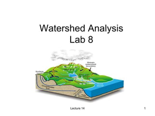
2. Basin
• Creates a raster delineating all drainage
basins.
• All cells in the raster will belong to a basin,
even if that basin is only one cell.
• The drainage basins are delineated within
the analysis window by identifying ridge
lines between basins.
• The input flow direction raster is analyzed
to find all sets of connected cells that
belong to the same drainage basin.
Lecture 14 2
3. • The drainage basins
are created by locating
the pour points at the
edges of the analysis
window (where water
would pour out of the
raster), as well as
sinks, then identifying
the contributing area
above each pour point.
This results in a raster
of drainage basins.
Lecture 14 3
4. Lab 8 Data
• Report Sheet is on the Website with the
instructions,
• Three files will be downloaded:
– 2 from NY Gis Clearinghouse
– 1 from Cornell University
• The DEM will be obtained from ArcGIS
online.
4
Lecture 14
6. Measuring in Arc-Seconds
Lecture 14 6
• Some USGS DEM data is stored in a
format that utilizes three, five, or 30 arc-
seconds of longitude and latitude to
register cell values.
• The geographic reference system treats
the globe as if it were a sphere divided into
360 equal parts called degrees.
7. • Each degree is subdivided into 60
minutes. Each minute is composed of 60
seconds.
• Arc-seconds of latitude remain nearly
constant, while arc-seconds of longitude
decrease in a trigonometric cosine-based
fashion as one moves toward the earth's
poles.
Lecture 14 7
8. Processing of DEM
• Raster clip – To the buffered park
boundry.
• Raster projection – from Geographic to
UTM Zone 18N, NAD83
• Resample – Bilinear Interpolation
• Change the cell size – from 30 second arc
to 30 meters,
8
Lecture 14
9. Raster Geometry and Resampling
• Data must often be resampled when
converting between coordinate systems
or changing the cell size of a raster data
set.
• Common methods:
– Nearest neighbor
– Bilinear interpolation
– Cubic convolution
9
Lecture 14
15. Sinks
• A sink is a cell or set of spatially connected cells
whose flow direction cannot be assigned one of
the eight valid values in a flow direction raster.
• This can occur when all neighboring cells are
higher than the processing cell or when two cells
flow into each other, creating a two-cell loop.
• To create an accurate representation of flow
direction and, therefore, accumulated flow, it is
best to use a dataset that is free of sinks.
• A digital elevation model (DEM) that has been
processed to remove all sinks is called a
depressionless DEM.
From ArcGIS 10 Desktop Help Lecture 14 15
16. High pass filters
Return:
•Small values when smoothly changing
values.
•Large positive values when centered on a
spike
•Large negative values when centered on a
pit
Lecture 14 16
20. Fill
• Fills sinks in a surface raster to remove
small imperfections in the data.
• Sinks (and peaks) are often errors due to
the resolution of the data or rounding of
elevations to the nearest integer value.
Lecture 14 20
26. Conditional
• The results of Flow Accumulation can be used to
create a stream network by applying a threshold
value to select cells with a high accumulated flow.
• For example, the procedure to create a raster
where the value 1 represents the stream network
on a background of NoData could use one of the
following:
• Perform a conditional operation with the Con tool
with the following settings:
– Input conditional raster : Flowacc
– Expression : Value > 50000
– Input true raster or constant : 1
From ArcGIS 10 Desktop Help
Lecture 14 26
28. Stream Link
• Assigns unique values to
sections of a raster linear
network between intersections.
• Links are the sections of a
stream channel connecting two
successive junctions, a junction
and the outlet, or a junction and
the drainage divide.
• Links are the sections of a
stream channel connecting two
successive junctions, a junction
and the outlet, or a junction and
the drainage divide.
From ArcGIS 10 Desktop Help Lecture 14 28
32. 32
Introduction
• Spatial data and analysis standards are
important because of the range of organizations
producing and using spatial data, and the
amount of data transferred between these
organizations.
• There are several types of standards:
– Data standards
– Interoperability standards
– Analysis standards
– Professional and certification standards
Lecture 14
33. 33
Introduction (continued)
• National and international standards
organizations are important in defining and
maintaining geospatial standards:
– Federal Geographic Data Committee (FGDC) which
focuses on the national spatial data infrastructure
(www.fgdc.gov)
– International Spatial Data Standards Commission
which is a clearing house and gateway for
international standards
– Open Geospatial Consortium (OGC) which is
developing interoperability standards. Web Mapping
Service (WMS) standards are an example.
Lecture 14
36. 36
36
GIS Professional Certification
URISA is the founding member of the GIS
Certification Institute, the organization that
administers professional certification for the field
and is dedicated to advancing the industry.
Education: 30 Points
Experience: 60 Points
Contributions: 8 Points
The additional 52 points can be counted from any of the three categories.
The minimum number of points needed to become a certified GIS
Professional as detailed in the three point schedules given below is 150
points. Thus, all applicants are expected to document achievements valued at a
minimum of 150 points. To ensure that applicants have a broad foundation, specific
minimums in each of the three achievement categories must be met or
exceeded. These minimums are as follows:
Lecture 14
38. 38
University Certificates
• UMM – undergraduate
• USM undergrad/grad
• UM – graduate
• Penn State – graduate
• University of Denver
• University of Southern California
• George Mason University
Lecture 14
39. 39
39
Spatial Data Standards
• Data – measurements and observations
• Data quality – a measure of the fitness for
use of data for a particular task (Chrisman,
1994).
• It is the responsibility of the user to insure
that the data is fit for the task.
• Metadata – data about the data
Lecture 14
40. 40
40
Spatial Data Standards
• Spatial Data Standards – methods for structuring,
describing and delivering spatially-referenced data.
• Media Standards – the physical form of the data
(CD/download etc).
• Format Standards – specify data file components
and structures. These standards aid in data
transfer.
• Spatial Data Accuracy Standards –document the
quality of the positional and attribute accuracy.
• Document Standards – define how we describe
spatial data.
Lecture 14
41. 41
41
GIS Is Not Perfect
A GIS cannot perfectly represent the world for many
reasons, including:
• The world is too complex and detailed.
• The data structures or models (raster, vector, or
TIN) used by a GIS to represent the world are not
discriminating or flexible enough.
• We make decisions (how to categorize data, how
to define zones) that are not always fully informed
or justified.
• It is impossible to make a perfect representation
of the world, so uncertainty is inevitable
• Uncertainty degrades the quality of a spatial
representation
Lecture 14
42. 42
42
Concepts Related to Data
Quality
• Related to individual data sets:
– Errors – flaws in data
– Accuracy – the extent to which an estimated
value approaches the true value.
– Precision – the recorded level of detail of your
data.
– Bias – the systematic variation of the data
from reality.
Lecture 14
44. 44
44
Concepts Related to Data
Quality
• Related to source data:
– Resolution – the smallest feature in the data
set that can be displayed.
– Generalization- simplification of objects in the
real world to produce scale models and maps.
Lecture 14
47. 47
47
Data Sets Used for Analysis
Must be:
– Complete – spatially and temporally
– Compatible – same scale, units of measure,
measurement level
– Consistent – both within and between data
sets.
– And Applicable for the analysis being
performed.
Lecture 14
48. 48
48
A Conceptual View of Uncertainty
Real World
Conception
Data conversion and Analysis
Source Data, Measurements &
Representation
Result
Lecture 14
49. 49
49
Uncertainty in The Conception of
Geographic Phenomena
Many spatial objects are not well defined or their
definition is to some extent arbitrary, so that people
can reasonably disagree about whether a particular
object is x or not. There are at least four types of
conceptual uncertainty
– Spatial uncertainty
– Vagueness
– Ambiguity
– Regionalization problems
Lecture 14
50. 50
50
Spatial uncertainty occurs when objects do not
have a discrete, well defined extent.
• They may have indistinct boundaries.
• They may have impacts that extend beyond
their boundaries.
• They may simply be statistical entities.
• The attributes ascribed to spatial objects may
also be subjective.
Spatial uncertainty
Lecture 14
51. 51
51
• Vagueness occurs when the criteria that
define an object as x are not explicit or
rigorous.
• For example:
– In a land cover analysis, how many oaks (or
what proportion of oaks) must be found in a
tract of land to qualify it as oak woodland?
– What incidence of crime (or resident
criminals) defines a high crime neighborhood?
Vagueness (obscureness)
Lecture 14
52. 52
52
Ambiguity
Ambiguity occurs when y is used as a substitute,
or indicator, for x because x is not available.
• The link between direct indicators and the
phenomena for which they substitute is
straightforward and fairly unambiguous (soil
nutrients for crop yield).
• Indirect indicators tend to be more ambiguous and
opaque (wetlands as an indicator of species
diversity).
• Of course, indicators are not simply direct or
indirect; they occupy a continuum. The more
indirect they are, the greater the ambiguity.
Lecture 14
53. 53
53
• Regional geography is largely founded on the
creation of a mosaic of zones that make it easy
to portray spatial data distributions.
• A uniform zone is defined by the extent of a
common characteristic, such as climate,
landform, or soil type.
• Functional zones are areas that delimit the
extent of influence of a facility or feature—for
example, how far people travel to a shopping
center or the geographic extent of support for a
football team.
• Regionalization problems occur because zones
are artificial.
Regionalization problems
Lecture 14
54. 54
54
Uncertainty in the measurement of
geographic phenomena
Error occurs in physical measurement of
objects. This error creates further
uncertainty about the true nature of spatial
objects.
– Physical measurement error
– Digitizing error
– Error caused by combining data sets with
different lineages
Lecture 14
55. 55
55
Physical measurement error
• Instruments and procedures used to make
physical measurements are not perfectly
accurate.
• In addition, the earth is not a perfectly stable
platform from which to make measurements.
Seismic motion, continental drift, and the
wobbling of the earth's axis cause physical
measurements to be inexact. (GPSing error,
remote sensing error)
Lecture 14
56. 56
56
Digitizing Error
A great deal of spatial
data has been
digitized from paper
maps.
Any digitized map requires:
Considerable post-processing
Check for missing features
Connect lines
Remove spurious polygons
Some of these steps can be automated
Lecture 14
57. 57
57
Error caused by combining data
sets with different lineages
• Data sets produced by different agencies or vendors
may not match because different processes were
used to capture or automate the data.
– For example, buildings in one data set may appear on the
opposite side of the street in another data set.
– Error may also be caused by combining sample and
population data or by using sample estimates that are not
robust at fine scales.
– "Lifestyle" data are derived from shopping surveys and
provide business and service planners with up-to-date
socioeconomic data not found in traditional data sources
like the census. Yet the methods by which lifestyle data
are gathered and aggregated to zones or are compared to
census data may not be scientifically rigorous
58. 58
58
Uncertainty in the representation of
geographic phenomena
• Representation is closely related to measurement.
• Representation is not just an input to analysis, but
sometimes also the outcome of it. For this reason, we
consider representation separately from measurement.
– The world is infinitely complex, but computer system are finite.
– Representation is all about the choices that are made in capturing
knowledge about the world
– Uncertainty in earth model: ellipsoid models, datum, projection
types
– Uncertainty in the raster data model (structure)
– Uncertainty in the vector data model (structure)
Lecture 14
59. 59
59
• The raster structure partitions space into square cells of
equal size.
• Spatial objects x, y, and z emerge from cell classification, in
which Cell A1 is classified as x, Cell A2 as y, Cell A3 as z,
and so on, until all cells are evaluated.
• A spatial object x can be defined as a set of contiguous cells
classified as x.
• But not all the area covered by the cell is x
• These impure cells are termed mixed pixels or "mixels."
• Because a cell can hold only one value, a mixel must be
classified as if it were all one thing or another. Therefore, the
raster structure may distort the shape of spatial objects.
Uncertainty in the raster data
structure
Lecture 14
60. 60
Raster – The Mixed Pixel Problem
Landcover map –
Two classes, land or
water
Cell A is
straightforward
What category to
assign
For B, C, or D?
Lecture 14
61. 61
61
Error in raster
• raster
- because of the distortions due to flattening, cells in a raster can never be
perfectly equal in size on the Earth’s surface.
- when information is represented in raster form all detail about variation within
cells is lost, and instead the cell is given a single value. largest share, central
point (f.g. USGS DEM), and mean value (f.g. remote sensing imagery)
Largest share
Central point
8
6 7.5
Mean value
6.33
6
6.29
8
8
8 6
6
6
6
6
8x(1/6)+6x(5/6)=6.33
8x(3/4)+6x(1/4)=7.5
8x(1/7)+6x(6/7)=6.29
Lecture 14
62. 62
62
Figure 10.8 Problems with remotely sensed imagery: (left) example of a satellite image
with cloud cover (A), shadows from topography (B), and shadows from cloud cover
(C); (right) an urban area showing a building leaning away from the camera
Source: Ian Bishop (left) and Google UK (right)
Lecture 14
63. 63
63
• Socioeconomic data—facts about people, houses,
and households—are often best represented as
points.
• For various reasons (to protect privacy, to limit data
volume), data are usually aggregated and reported
at a zonal level, such as census tracts or ZIP
Codes.
• This distorts the data in two ways:
– First, it gives them a spatially inappropriate representation
(polygons instead of points);
– Second, it forces the data into zones whose boundaries
may not respect natural distribution patterns.
Uncertainty in the vector data
structure
Lecture 14
64. 64
64
Map scale Ground distance, accuracy, or resolution
(corresponding to 0.5 mm map distance)
1:1,250 0.625 m
1:2,500 1.25 m
1:5,000 2.5 m
1:10,000 5 m
1:24,000 12 m
1:50,000 25 m
1:100,000 50 m
1:250,000 125 m
1:1,000,000 500 m
1:10,000,000 5 km
Lecture 14
Map Representation Error
65. 65
65
Uncertainty in the data conversion and
analysis of geographic phenomena
Uncertainties in data lead to uncertainties in the results of
analysis; Data conversion and spatial analysis methods
can create further uncertainty
• Data conversion error
• Georeferencing and resampling
• Projection and datum conversions
• The ecological fallacy
• The modifiable areal unit problem (MAUP)
• Classification errors
Lecture 14
71. 71
71
Confusion Matrix
1686
Grass Alfalfa Cotton Chili Fallow
(corn)
total User
accuracy (%)
Grass 110 22 0 0 0 132 83.3
Alfalfa 5 105 0 0 0 110 79.5
Cotton 0 0 945 5 0 950 99.5
Chili 0 0 50 42 0 92 45.7
Fallow 0 0 0 0 484 484 100
total 115 127 995 47 484 1768
Producer
accuracy (%)
95.6 82.7 95.0 89.4 100
G
r
o
u
n
d
t
r
u
t
h
%
4
.
95
1768
1686
_
Accuracy
Overlay
%
3
.
89
1768
/
)
484
484
47
92
995
950
127
110
115
132
(
1768
1768
/
)
484
484
47
92
995
950
127
110
115
132
(
1686
_
x
x
x
x
x
x
x
x
x
x
Index
Kappa Lecture 14
72. 72
72
• Producer accuracy is a measure indicating the probability
that the classifier has labeled an image pixel into Class A
given that the ground truth is Class A.
• User accuracy is a measure indicating the probability that a
pixel is Class A given that the classifier has labeled the
pixel into Class A
• Overall accuracy is total classification accuracy.
• Kappa index (another parameter for overall accuracy) is a
more useful index for evaluating accuracy.
– Errors of commission represent pixels that belong to another class
but are labeled as belonging to the class.
– Errors of omission represent pixels that belong to the ground truth
class but that the classification technique has failed to classify them
into the proper class.
Bases of Confusion Matrix
Lecture 14
73. 73
73
Finding and Modeling Errors
• Checking for errors
– Visual inspection during data editing and
cleaning.
– Attributes can be checked by using
annotation, line colors and patterns.
– Double digitizing
– Statistical analysis may identify extreme
values of attributes.
Lecture 14
74. 74
74
Finding and Modeling Errors
• Error modeling
– 1. Epsilon modeling
• Based on a method of line generalization, and
adapted by Blakemore.
• It places an error band around a digitized line,
describing the probable distribution of error.
• Error distribution is subject to debate:
– Normal curve
– Piecewise quartile distribution
– Bimodal
• The epsilon band can be used in analyses to
improve the confidence of the user in the result.
Lecture 14
76. 76
76
Finding and Modeling Errors
• Error modeling
– 2. Monte Carlo simulation – used in
overlays.
• Simulates input data error by adding random noise
to the line coordinates of the map data.
• Each input is assumed to be characterized by an
estimate of positional error.
• This changes the shape of the line.
• The process is repeated multiple times and the
randomized data put through the GIS analyses.
• Output:
– A number
– A map
Lecture 14
78. 78
78
Managing GIS Error
• To manage errors we must track and
document them.
• The concepts introduced earlier:
– Accuracy, Precision, Resolution,
Generalization, Bias, Compatibility,
Completeness and Consistency
provide a checklist of quality indicators:
• These should be documented for each
data layer.
Lecture 14
79. 79
79
Managing GIS Error
• Data quality information can be used to
create a data lineage.
• A record of the data history that presents
essential information about the
development of the data.
• This becomes the metadata.
Lecture 14
80. 80
80
Living with uncertainty
• uncertainty is inevitable and easier to find,
• use metadata to document the uncertainty
• sensitivity analysis to find the impacts of input
uncertainty on output,
• rely on multiple sources of data,
• be honest and informative in reporting the results of GIS
analysis.
• US Federal Geographic Data Committee lists five
components of data quality: attribute accuracy,
positional accuracy, logical consistency, completeness,
and lineage (details see www.fgdc.gov)
Lecture 14
81. 81
81
Basics of FGDC
• Federal Geographic Data Committee
(FGDC) metadata answers the who, what,
where, when, how and why questions of
geospatial data.
• The data structure and elements defined
for FGDC metadata are described fully in
the “Content Standard for Digital
Geospatial Metadata” (CSDGM).
Lecture 14
82. 82
82
SEVEN SECTIONS OF FGDC
The Federal Geographic Data Committee
(FGDC), Content Standard for Digital Geospatial
Metadata (CSDGM) organizes a metadata
record into seven main sections:
– Identification Information
– Data Quality Information
– Spatial Data Organization Information
– Spatial Reference Information
– Entity and Attribute Information
– Distribution Information
– Metadata Reference Information
Lecture 14
83. 83
83
Lecture 14
Identification Information
• What is the name of the dataset?
• What is the subject or theme of the information included?
• What is the scale of the dataset?
• What are the attributes of the dataset?
• Where is the geographic location of the dataset?
• Who developed the dataset?
• Who provided the source material for the dataset?
• Who will publish the dataset?
• When were the features of the dataset identified?
• How are the features of the dataset depicted?
• Why was the data set created?
• Are there restrictions on accessing or using the data?
• Are external files available that are related to the dataset?
84. 84
84
Lecture 14
Data Quality Information
• How reliable are the data?
• What are its limitations or inconsistencies?
• What is the positional and attribute accuracy?
• Is the dataset complete?
• Were the consistency and content of the data
verified?
• Where can the sources of the data be located?
• What processes were applied to these sources
and by whom?
85. 85
85
Lecture 14
Spatial Data Organization
• What spatial data model was used to
encode the spatial data?
• How many and what kind of spatial objects
are included in the dataset?
• Are methods other than coordinates, such
as street addresses used to encode
locations?
86. 86
86
Lecture 14
Spatial Reference
• Are coordinate locations encoded using
longitude and latitude?
• What map projections is used?
• What horizontal datum and/or vertical
datum are used?
• What parameters should be used to
convert the data to another coordinate
system?
87. 87
87
Lecture 14
Entity and Attribute Information
• What geographic information (roads,
houses, elevation, temperature, etc.) is
described?
• How is this information coded?
• What do the codes mean?
• What source was used for defining the
attributes or codes, i.e. Cowardin
classification?
88. 88
88
Lecture 14
Distribution
• From whom can the data be obtained?
• What formats are available?
• What media are available?
• Are the data available online?
• What is the price of the data?
89. 89
89
Lecture 14
Metadata Reference
• When were the metadata compiled, and
by whom?
• When was the metadata record created?
• Who is the responsible party?
• When were the metadata last updated?