
Recommended
More Related Content
Similar to Models of Causal RelationshipsDrawing upon the concepts presente.docx
Similar to Models of Causal RelationshipsDrawing upon the concepts presente.docx (20)
More from roushhsiu
More from roushhsiu (20)
Recently uploaded
Recently uploaded (20)
Models of Causal RelationshipsDrawing upon the concepts presente.docx
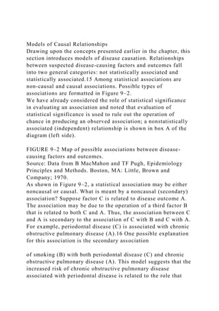
- 1. Models of Causal Relationships Drawing upon the concepts presented earlier in the chapter, this section introduces models of disease causation. Relationships between suspected disease-causing factors and outcomes fall into two general categories: not statistically associated and statistically associated.15 Among statistical associations are non-causal and causal associations. Possible types of associations are formatted in Figure 9–2. We have already considered the role of statistical significance in evaluating an association and noted that evaluation of statistical significance is used to rule out the operation of chance in producing an observed association; a nonstatistically associated (independent) relationship is shown in box A of the diagram (left side). FIGURE 9–2 Map of possible associations between disease- causing factors and outcomes. Source: Data from B MacMahon and TF Pugh, Epidemiology Principles and Methods. Boston, MA: Little, Brown and Company; 1970. As shown in Figure 9–2, a statistical association may be either noncausal or causal. What is meant by a noncausal (secondary) association? Suppose factor C is related to disease outcome A. The association may be due to the operation of a third factor B that is related to both C and A. Thus, the association between C and A is secondary to the association of C with B and C with A. For example, periodontal disease (C) is associated with chronic obstructive pulmonary disease (A).16 One possible explanation for this association is the secondary association of smoking (B) with both periodontal disease (C) and chronic obstructive pulmonary disease (A). This model suggests that the increased risk of chronic obstructive pulmonary disease associated with periodontal disease is related to the role that
- 2. smoking may play as a cofactor in both conditions. Here is a map of a secondary association: C ← B → A.1 With respect to causal associations, the relationship between factor and outcome may be indirect or direct. An indirect causal association involves the operation of an intervening variable, which is a variable that falls in the chain of association between C and A. An illustration of an indirect association is the postulated relationship between low education levels (C) and obesity (A) among men.17 Men who have lower education levels tend to be more obese than those who have higher education levels. It is plausible that the relationship between C and A operates through the intervening variable of lack of leisure time physical activity (B). An indirect association involves an intervening variable in the association between C and A. This relationship may be formatted as follows: C → B → A.1 Note that the arrow between C and B has been reversed in contrast with an indirect noncausal association. Multiple Causality The foregoing section provided models of causality that employ more than one factor. As stated earlier in this chapter, the measure risk difference implies multivariate causality by isolating the effects of a single exposure from the effects of other exposures. The example on NSAIDs examined the difference between risk of peptic ulcer among users and nonusers of NSAIDs, where the risk difference was 12.5 per 1,000 person-years. The risk of peptic ulcer caused by other exposures was 4.2 per 1,000 person-years. The issue of disease causality is exceedingly complicated. To describe exposure–disease relationships, epidemiologists have developed complex models of disease causality. These models acknowledge the multifactor causality of diseases, even those that seem to have “simple” infectious agents. Often, these models involve an ecologic approach by relating disease to one or more environmental factors. “The requirement that more than
- 3. one factor be present for disease to develop is referred to as multiple causation or multifactorial etiology.”18(p 27) Examples of several influential models are the: · •• epidemiologic triangle · •• web of causation · •• wheel model · •• pie model Web of causation The web of causation is “… a popular METAPHOR for the theory of sequential and linked multiple causes of diseases and other health states.”1 The web of causation implicates broad classes of events and represents an incomplete portrayal of reality.15 Although the web of causation for most diseases is complex, one may not need to understand fully the causality of any specific disease in order to prevent it. An example of the web of causation of avian influenza is provided in Figure 9–3. Follow the infection of the human host from the virus reservoir in wild birds. As of 2007, the virus had not mutated into a form that could be spread readily from person to person. Wheel model The wheel model is similar to the epidemiologic triangle and web of causation with respect to involving multiple causality (Figure 9–4). Observe that the model explains the etiology of disease by calling into play host and environment interactions. Environmental components are biologic, social, and physical. The circle designated as “host” refers to human beings or other hosts affected by a disease. The circle called “genetic core” acknowledges the role that genetic factors play in many diseases. The wheel model de-emphasizes specific agent factors and, instead, differentiates between host and environmental factors in disease causation. The biologic environment is relevant to infectious agents, by taking into account the environmental dimensions that permit survival of microbial agents of disease.
- 4. FIGURE 9–3 The web of causation for avian influenza. A wheel model may be used to account for the occurrence of childhood lead poisoning.18 In this example, preschool children are typical hosts. The physical environment provides many opportunities for lead exposure from lead-based paint in older homes, playground equipment, candy wrappers, and other sources. Some children ingest paint chips from peeling surfaces as a result of pica, the predilection to eat nonfood substances. Because lead-based paints often are located in poorer neighborhoods that have substandard housing, the social environment is associated with childhood poisoning. Limited access to medical care in such communities may restrict screening of preschool children for lead exposure. Elimination of childhood lead poisoning requires visionary public health leadership to advocate for detection of lead-based paints and other sources of environmental lead exposure as well as the implementation of screening programs. Such efforts will help to protect vulnerable children against the sequelae of lead poisoning. Pie model Another model of multiple causality (multicausality) is the causal pie model.19 As Figure 9–5 shows, the model indicates that a disease may be caused by more than one causal mechanism (also called a sufficient cause), which is defined as “a set of minimal conditions and events that inevitably produce disease.”19(p S144) Each causal mechanism is denoted in Figure 9–5 by the numerals I through III. An example of different causal mechanisms for a disease is provided by the etiology of lung cancer: lung cancer caused by smoking; lung cancer caused by exposure to ionizing radiation; and lung cancer caused by inhalation of carcinogenic solvents in the workplace. FIGURE 9–5 Three sufficient causes of disease.
- 5. Source: From KJ Rothman and S Greenland, Causation and causal inference in epidemiology, Am J Public Health, 2005; vol 95, p S145. Reprinted with permission from the American Public Health Association. Rothman and Greenland note that, “A given disease can be caused by more than one causal mechanism, and every causal mechanism involves the joint action of a multitude of component causes.”19(p S145) The component causes, or factors, are denoted by the letters shown within each pie slice. A single letter indicates a single component cause. A single component could be common to each causal mechanism (shown by the letter A that appears in each pie); in other cases, the component causes for each causal mechanism could be different for each mechanism (shown by the letters that differ across the pies). Returning to the lung cancer example, a common factor that could apply to all causal mechanisms for lung cancer is a genetic predisposition for cancer. Several other component causes might be different for each causal mechanism involved in the etiology of lung cancer. In models of multicausality, most of the identified component causes are neither necessary nor sufficient causes (defined in the section on absolute effects). Accordingly, it is possible to prevent disease when a specific component cause that is neither necessary nor sufficient is removed; nevertheless, when the effects of this component cause are removed, cases of the disease will continue to occur. Conclusion This chapter covered two new measures of effect—absolute and relative effects—that may be used as aids in the interpretation of epidemiologic studies. In addition, the chapter presented guidelines that should be taken into account when one is interpreting an epidemiologic finding. Absolute effects, the first variety of which is called risk differences, are determined by finding the difference in measures of disease frequency between exposed and nonexposed individuals. A second type of absolute
- 6. effect, called population risk difference, is found by computing the difference in measures of disease frequency between the exposed segment of the population and the total population. Relative effects are characterized by the inclusion of an absolute effect in the numerator and a reference group in the denominator. One type of relative effect, the etiologic fraction, attempts to quantify the amount of a disease that is attributable to a given exposure. The second type of relative effect, the population etiologic fraction, provides an estimate of the possible impact on the population rates of disease that can be anticipated by removal of the offending exposure. With respect to interpretation of epidemiologic findings, one should be cognizant of the influence of sample size upon the statistical significance of the results. Large sample sizes may lead to clinically unimportant, yet statistically significant, results; small sample sizes may yield statistically nonsignificant results that are clinically important. Therefore, we presented a series of five questions that should be asked when one attempts to interpret an epidemiologic observation. The chapter closed with a discourse on causal models, which may be particularly instructive when trying to interpret epidemiologic data. DATAProductAgeGenderEducationMarital StatusUsageFitnessIncomeMilesTM19518Male14Single3429562 112TM19519Male15Single233183675TM19519Female14Partner ed433069966TM19519Male12Single333297385TM19520Male13 Partnered423524747TM19520Female14Partnered333297366TM 19521Female14Partnered333524775TM19521Male13Single3332 97385TM19521Male15Single5435247141TM19521Female15Par tnered233752185TM19522Male14Single333638485TM19522Fe male14Partnered323524766TM19522Female16Single433638475 TM19522Female14Single333524775TM19523Male16Partnered3 13865847TM19523Male16Partnered334093275TM19523Female 14Single2334110103TM19523Male16Partnered433979594TM19 523Female16Single4338658113TM19523Female15Partnered223
- 9. Single4548556200TM79823Male16Single4558516140TM79823 Female18Single5453536100TM79823Male16Single4548556100 TM79824Male16Single4561006100TM79824Male18Partnered45 5727180TM79824Female16Single5552291200TM79824Male16S ingle5549801160TM79825Male16Partnered4549801120TM7982 5Male16Partnered4462251160TM79825Female18Partnered5561 006200TM79825Male18Partnered4364741100TM79825Male18P artnered6470966180TM79825Male18Partnered6575946240TM7 9825Male20Partnered4574701170TM79826Female21Single4369 721100TM79826Male16Partnered5464741180TM79827Male16P artnered4583416160TM79827Male18Single4388396100TM7982 7Male21Partnered4490886100TM79828Female18Partnered6592 131180TM79828Male18Partnered7577191180TM79828Male18S ingle6588396150TM79829Male18Single5552290180TM79829M ale14Partnered7585906300TM79830Female16Partnered6590886 280TM79830Male18Partnered54103336160TM79830Male18Part nered5599601150TM79831Male16Partnered6589641260TM798 33Female18Partnered4595866200TM79834Male16Single559213 1150TM79835Male16Partnered4592131360TM79838Male18Part nered55104581150TM79840Male21Single6583416200TM79842 Male18Single5489641200TM79845Male16Single5590886160T M79847Male18Partnered45104581120TM79848Male18Partnere d4595508180 ADMN 210 – Dr. Barbara Sirotnik Case #2 of 3, Summer 2019 In the last case you reviewed chapters 1 – 3 material and also applied your knowledge of chapter 8 material (estimation). I’d like for you to use the same dataset, but this time apply chapter 9 material (hypothesis testing). As a reminder: On page 28 – 29 of your text you will find the description of a data set for a company that sells three different levels of treadmills (as well as other exercise equipment).
- 10. 1) Download a clean copy of the file CardioGoodFitness.xlsx to your computer.Remember, don’t try to work on it by just clicking on the file name from Blackboard. You need to save it first. 2) Years ago the company did an analysis of their entire customer base and found that the average income for their customers was $50,000. They believe that incomes of their current customers are significantly higher than that. Test at the 10% significance level, showing all steps of the hypothesis testing procedure (see the text, page 307). Be sure to include a practical statement indicating how the company could use the results you’ve found. HINT: here are the steps to follow… · Write your Ho and H1 · Make note of your alpha (level of significance) · Determine your test statistic (that is, find the proper formula to use) · Find the critical value of the test statistic from the table, and define your rejection region · Find your sample mean and standard deviation using the proper Excel formulas. Compute the value of the test statistic (that is, do the number crunching in the formula you identified in the third step) · Make the statistical decision and interpret in practical form 3) Years ago about 30% of purchases were for the TM 798 (the “high end” expensive treadmill), however since those data were collected we’ve gone through a recession, and a lot of people’s finances haven’t really recovered. Has the proportion of people purchasing the TM 798 dropped significantly? Test at the 5% level of significance. Be sure to include a practical statement indicating how the company could use the results you’ve found. That’s it! The final case (for chapter 13) will use the same data set but will focus on relationships between variables.