The Apriori algorithm is used to find frequent itemsets and association rules in transactional datasets. It employs an iterative, level-wise approach where frequent itemsets of length k are used to generate candidate itemsets of length k+1. The algorithm exploits the Apriori property which states that all nonempty subsets of a frequent itemset must also be frequent. This helps reduce the search space and improves efficiency. The algorithm outputs frequent itemsets and association rules with support and confidence above predefined thresholds.

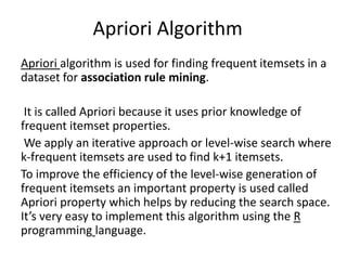
1. Apriori Algorithm
Apriori algorithm is used for finding frequent itemsets in a
dataset for association rule mining.
It is called Apriori because it uses prior knowledge of
frequent itemset properties.
We apply an iterative approach or level-wise search where
k-frequent itemsets are used to find k+1 itemsets.
To improve the efficiency of the level-wise generation of
frequent itemsets an important property is used called
Apriori property which helps by reducing the search space.
It’s very easy to implement this algorithm using the R
programming language.

2. • Apriori Property: All non-empty subsets of a
frequent itemset must be frequent. Apriori
assumes that all subsets of a frequent itemset
must be frequent (Apriori property). If an itemset
is infrequent, all its supersets will be infrequent.

3. • Essentially, the Apriori algorithm takes each part of a
larger data set and contrasts it with other sets in some
ordered way. The resulting scores are used to generate
sets that are classed as frequent appearances in a larger
database for aggregated data collection.
• In a practical sense, one can get a better idea of the
algorithm by looking at applications such as a Market
Basket Tool that helps with figuring out which items are
purchased together in a market basket, or a financial
analysis tool that helps to show how various stocks trend
together.
• The Apriori algorithm may be used in conjunction with
other algorithms to effectively sort and contrast data to
show a much better picture of how complex systems
reflect patterns and trends.

4. • Important Terminologies
• Support: Support is an indication of how frequently the itemset
appears in the dataset. It is the count of records containing an item
‘x’ divided by the total number of records in the database.
• Confidence: Confidence is a measure of times such that if an item
‘x’ is bought, then item ‘y’ is also bought together. It is the support
count of (x U y) divided by the support count of ‘x’.
• Lift: Lift is the ratio of the observed support to that which is
expected if ‘x’ and ‘y’ were independent. It is the support count of
(x U y) divided by the product of individual support counts of ‘x’ and
‘y’.
• Algorithm
• Read each item in the transaction.
• Calculate the support of every item.
• If support is less than minimum support, discard the item. Else,
insert it into frequent itemset.
• Calculate confidence for each non- empty subset.
• If confidence is less than minimum confidence, discard the subset.
Else, it into strong rule

5. • install.packages("arules")
• library(arules)
• Super<-read.csv("E:/MCA II Year Data/Super.csv", header = T,colClasses = "factor")
• Super
• summary(Super)
• View(Super)
• dim(Super)
• length(Super)
• #find association
• rules<-apriori(Super)
• #produce association support and confidence
• rules<-apriori(Super,parameter = list(supp=0.22,conf=.7))
• inspect(rules)
• #set max and minimun length of rules
• rules<-apriori(Super, parameter = list(minlen=2,maxlen=5,supp=.22,conf=.7))
• inspect(rules)
• #Remove all null
• rules<-apriori(Super, parameter = list(minlen=2,maxlen=5,supp=.22,conf=.7),
appearance = list(none=c("I1=No","I2=No","I3=No","I4=No","I5=No")))
• inspect(rules)

6. • #Select items in antendent and consequent
• rules<-apriori(Super, parameter =
list(minlen=2,maxlen=5,supp=.22,conf=.7), appearance =
list(none=c("I1=No","I2=No","I3=No","I4=No","I5=No"),lhs=c("I1=Yes","I5=
Yes"),rhs=c("I2=Yes")))
• inspect(rules)
• #round off to 3 afterdecimal point
• quality(rules)<-round(quality(rules),digits = 3)
• quality(rules)
• inspect(rules)
• #writing rules into CSV file
• write(rules,file ="E:/MCA II Year Data/rk.csv",sep="," )
• #ploting the graph
• install.packages("arulesViz")
• library(arulesViz)
• plot(rules)#scatter plot
• plot(rules,method = "grouped")
• plot(rules,method = "graph",control = list(type="items"))

7. • Example:
• Step 1: Load required library
• ‘arules’ package provides the infrastructure for
representing, manipulating, and analyzing transaction data
and patterns.
• library(arules)’arulesviz’ package is used for visualizing
Association Rules and Frequent Itemsets. It extends the
package ‘arules’ with various visualization techniques for
association rules and itemsets. The package also includes
several interactive visualizations for rule exploration.
• library(arulesViz)‘RColorBrewer‘ is a ColorBrewer Palette
which provides color schemes for maps and other graphics.
• library(RColorBrewer)

8. • Step 2: Import the dataset
• ‘Groceries‘ dataset is predefined in the R package. It is a set
of 9835 records/ transactions, each having ‘n’ number of
items, which were bought together from the grocery store.
• data("Groceries")
• Step 3: Applying apriori() function
• ‘apriori()‘ function is in-built in R to mine frequent itemsets
and association rules using the Apriori algorithm. Here,
‘Groceries’ is the transaction data. ‘parameter’ is a named
list that specifies the minimum support and confidence for
finding the association rules. The default behavior is to mine
the rules with minimum support of 0.1 and 0.8 as the
minimum confidence. Here, we have specified the minimum
support to be 0.01 and the minimum confidence to be 0.2.

9. • Step 4: Applying inspect() function
• inspect() function prints the internal
representation of an R object or the result of
an expression. Here, it displays the first 10
strong association rules.
• inspect(rules[1:10])

10. • Step 5: Applying itemFrequencyPlot() function
• itemFrequencyPlot() creates a bar plot for item
frequencies/ support. It creates an item
frequency bar plot for inspecting the distribution
of objects based on the transactions. The items
are plotted ordered by descending support. Here,
‘topN=20’ means that 20 items with the highest
item frequency/ lift will be plotted.
• arules::itemFrequencyPlot(Groceries, topN = 20,
col = brewer.pal(8, 'Pastel2'), main = 'Relative
Item Frequency Plot', type = "relative", ylab =
"Item Frequency (Relative)")

11. • # Loading Libraries
• library(arules)
• library(arulesViz)
• library(RColorBrewer)
•
• # import dataset
• data("Groceries")
•
• # using apriori() function
• rules <- apriori(Groceries,
• parameter = list(supp = 0.01, conf = 0.2))
•
• # using inspect() function
• inspect(rules[1:10])
•
• # using itemFrequencyPlot() function
• arules::itemFrequencyPlot(Groceries, topN = 20,
• col = brewer.pal(8, 'Pastel2'),
• main = 'Relative Item Frequency Plot',
• type = "relative",
• ylab = "Item Frequency (Relative)")

12. • If hard cheese is bought, then whole milk is
also bought.
• If buttermilk is bought, then whole milk is also
bought with it.
• If buttermilk is bought, then other vegetables
are also bought together.
• Also, whole milk has high support as well as a
confidence value.