The document discusses pathfinding in games, focusing on algorithms used for navigating non-player characters and units in various gaming genres. It outlines space representation techniques, including data structures like grids and graphs, and explores several algorithms, comparing their efficiencies, such as breadth-first search, depth-first search, Dijkstra's, and A*. Additionally, it addresses challenges related to dynamic changes in the game environment and coordinating multiple units for movement.

2. Hi,
This is Adrian
I am here because I love to build games and also
to give presentations. Today’s is about...

3. Pathfinding
in games

4. Our goal
Reach a target as well as possible.

5. Artificial intelligence
Non-player character (FPS)
Armies of units (RTS)
Enemies (Tower Defense)
Use cases
Player exploration
Objective display
GPS (Racing)

6. RTS Starcraft 2

7. Racing Test Drive Unlimited 2

8. RPG Mass Effect 2

9. Get objec
positio
Basic repetitive procedure
Close object
to target
Estimate
distance
to target
Get object
positione object
o target

10. 1.
Space representation
Data structures

11. Grid
Each cell is denoted by its row and column.
1, 1 1, 2 1, 3 1, 4 1, 5 1, 6 1, 7
2, 1 2, 2 2, 3 2, 4 2, 5 2, 6 2, 7
3, 1 3, 2 3, 3 3, 4 3, 5 3, 6 3, 7

12. Graph
Node are connected through edges.
1
3
2
6
5
8
4
7

13. Convex polygons
Convex = all segments with extremities inside lie inside.

14. 2.
Space manipulation
Algorithms

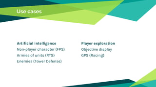
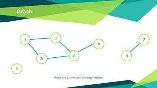
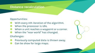
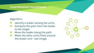
15. Random backstepping
Take one step in the direction of
the target. Avoid obstacles by
taking a step back.
Simple algorithms
Obstacle tracing
Similar to random
backstepping, calculates the
collision before it happens.

16. Advanced algorithms
◆ Breadth-first search (BFS)
◆ Depth-first search (DFS)
◆ Best-first search
◆ Dijkstra’s algorithm
◆ A* algorithm

17. BFS vs DFS
BFS is wide; DFS is deep.

18. Worst-case
space complexity
Worst-case
time complexity
Implementation
BFS vs DFS
Small: linear in the length
of the current path.
Large: linear in the area of
the explored surface, as it
explores useless paths.
By using a first-in,
first-out (FIFO) data
structure, e.g., a stack.
DFS
Large: linear in the
perimeter of the explored
surface.
Small: quadratic in the
length of the minimum
path.
By using a last-in, first out
(LIFO) data structure, e.g.,
a queue.
BFS

19. Dijkstra’s algorithm
◆ Solves the single-source shortest path problem.
◆ Invented by Edsger Dijkstra, Turing award winner.
◆ Used in many games for efficient pathfinding.
◆ More efficient than BFS and DFS in terms of time.
◆ More complex in implementation too.

20. Dijkstra pseudocode
◆ Start with two sets of graph nodes S and T.
◆ S contains the source node and T all others.
While the target node is not in S, do:
◆ Find the node in T that is closest to a node in S.
◆ Move that node from T to S.
◆ Relax the edges from the node to T.

21. Dijkstra efficiency
◆ To find the closest node, one can use an efficient data
structure, such as a simple heap, to answer queries for
the minimum in a totally-ordered set.
◆ Its operations take worst-case O(n) time, where n is the
number of nodes. With a simple heap, the worst-case
time complexity is O(m ⨉ log n), where m is the number of
edges.
◆ By using Fibonacci heaps, one can reduce the time
complexity down to O(m + n ⨉ log n), as m >> n.

22. A* algorithm
◆ A “combination” of BFS and Dijkstra.
◆ Does not use exact distances between nodes.
◆ Estimates the distance by using a heuristic.
◆ The heuristic should not overestimate the distance.
Possible heuristics:
◆ Manhattan distance - go straight, no diagonals.
◆ Diagonal distance - go only 45 deg. diagonals.
◆ Euclidean distance - distance in the plane.

23. A* traversal
The A* will visit the heuristically closest nodes to the target.

24. 3.
Dynamic changes
What about updates on the world?

25. Distance recalculation
Opportunities:
◆ With every nth iteration of the algorithm.
◆ When the processor is idle.
◆ When a unit reaches a waypoint or a corner.
◆ When the “near world” has changed.
Challenges:
◆ Previously computed data is thrown away.
◆ Can be show for large maps.

26. Path splice
Main idea:
◆ Splice the large path into smaller
paths.
◆ Only recalculate one or more of
the smaller paths.
◆ Handle the coordination of
multiple units - see image.
Challenges:
◆ Responds poorly to large changes.

27. Region partition
Main idea:
◆ Partition the map into regions.
◆ Each unit depends of a
specific region.
◆ Propagate a change only
within the region.
Challenges:
◆ Responds badly to large
changes - see image.

28. Obstacle prediction
Main idea:
◆ Incorporate heuristics that
predict how obstacles will move in
the future - see image.
Challenge:
◆ Depending on the game, the move
may be easy, hard, or impossible
to predict.

29. 4.
Multiple units
How can we coordinate them?

30. Individual movement
Algorithm:
◆ Find the center of a set of units.
◆ Compute the path from the center
to the target.
◆ Move each individual unit in
parallel, along the path - see
image.

31. Coordinated movement
Algorithm:
◆ Identify a leader among the units.
◆ Compute the path from the leader
to the target.
◆ Move the leader along the path.
◆ Make the other units flock around
the leader unit - see image.

32. Thank you.
Any questions?
You can find me at @dumitrix