This document provides an overview of structural deflections and methods for calculating beam deflection. It discusses how deflections are an important part of structural analysis and excessive deflections can lead to failures. The deflection curve of a beam is described as the initially straight axis bending into a curve. Methods for determining the deflection curve including drawing shear and moment diagrams and identifying the concave upward and downward portions. Examples are provided to demonstrate calculating deflection curves for various beams. The double integration method for relating beam deflections to bending moments is described. Assumptions and limitations of the method are also stated. Further examples demonstrate applying the double integration and moment-area methods to calculate maximum deflections in beams.

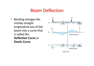
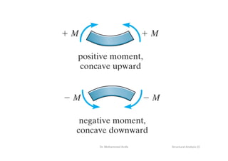
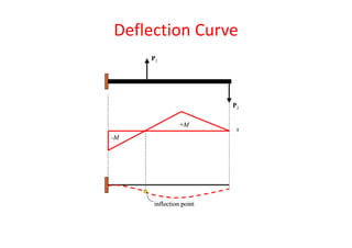
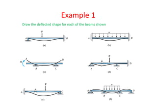
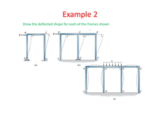
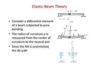
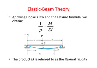
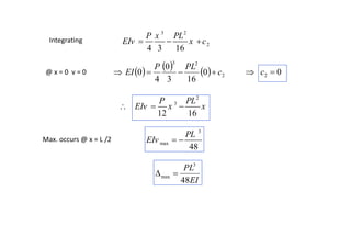
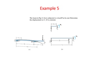
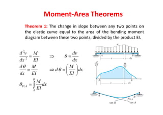
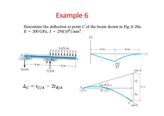
1. Structure Analysis I
Chapter 8
Structure Analysis I
Chapter 8

2. Deflections
Structural Analysis (I)Dr. Mohammed Arafa

3. Introduction
• Calculation of deflections is an important part of
structural analysis
• Excessive beam deflection can be seen as a mode of
failure.
– Extensive glass breakage in tall buildings can be attributed
to excessive deflections
– Large deflections in buildings are unsightly (and unnerving)
and can cause cracks in ceilings and walls.
– Deflections are limited to prevent undesirable vibrations

4. Beam Deflection
• Bending changes the
initially straight
longitudinal axis of the
beam into a curve that
is called the
Deflection Curve or
Elastic Curve

5. Beam Deflection
• To determine the deflection curve:
– Draw shear and moment diagram for the beam
– Directly under the moment diagram draw a line for the
beam and label all supports
– At the supports displacement is zero
– Where the moment is negative, the deflection curve is
concave downward.
– Where the moment is positive the deflection curve is
concave upward
– Where the two curve meet is the Inflection Point

6. Structural Analysis (I)Dr. Mohammed Arafa

7. Deflection Curve

8. Deflection Curve

9. Deflection Curve

10. Example 1
Draw the deflected shape for each of the beams shown

11. Example 2
Draw the deflected shape for each of the frames shown

12. Double Integration Method
Structural Analysis (I)Dr. Mohammed Arafa

13. Elastic‐Beam Theory
• Consider a differential element
of a beam subjected to pure
bending.
• The radius of curvature  is
measured from the center of
curvature to the neutral axis
• Since the NA is unstretched,
the dx=d

14. Elastic‐Beam Theory
• Applying Hooke’s law and the Flexure formula, we
obtain:
EI
M


1
• The product EI is referred to as the flexural rigidity

15. Elastic‐Beam Theory
Since:
1
then:
( )
dx d
d dx
M
d dx Slope
EI
 






  
  
EI
M
dx
vd
solutionexact
dxdv
dxvd
EI
M
dxdv
dxvd





2
2
2
3
2
22
2
3
2
22
)(
/1
/
/1
/1

 From calculus books:

16. The Double Integration Method
Relate Moments to Deflections
EI
M
dx
vd
2
2
 
 dx
xEI
xM
dx
dv
x
)(
)(
 
 2
)(
)( dx
xEI
xM
xv
Use Boundary Conditions to
Evaluate Integration
Constants
Structural Analysis (I)Dr. Mohammed Arafa

17. Assumptions and Limitations
• Deflections caused by shearing action negligibly
small compared to bending
• Deflections are small compared to the cross‐
sectional dimensions of the beam
• All portions of the beam are acting in the elastic
range
• Beam is straight prior to the application of loads

18. Example 1
PL
L
x
x
y
P
P
2
2
d v
EI M
dx
M PL Px

  
   
 
   
 
2
2
2
1
2
1 1
2 3
2
3
2
2 2
2 3
max
2
max
Integrating once:
2
0
@ 0, 0 0 0 0
2
Integrating twice:
2 6
0
@ 0, 0 0 0 0
2 6
@
2 6
2
d v
EI PL Px
dx
dv x
EI PLx P c
dx
dv
x EI PL P c c
dx
PLx x
EIv P c
PL
x v EI P c c
PLx x
EIv P x L v v
PL L
EIv
  
   
        
   
        
     
  
3 3 3
max
6 3 3
L PL PL
P v
EI
    

19. y
 2
2
xL
W
M 
2
2
d v
EI M
dx

@ x
 
2
2
2
2
d v W
EI L x
dx
  
Integrating once
 
3
1
2 3
L xdv W
EI c
dx

 
@ x = 0  
 
3 3
1 1
0
0 0
2 3 6
Ldv W WL
EI c c
dx

      
L
x
x
WL
W
2
2
WL
 
3
3
6 6
dv W WL
EI L x
dx
   
Example 2

20.  
3 4
4
24 6 24
W WL WL
EIv L x x    
Max. occurs @ x = L
4 4 4 4
max max
6 24 8 8
W L WL WL WL
EIv v
EI
       
EI
WL
8
4
max 
Integrating twice
 
4 3
2
6 4 6
L xW WL
EIv x c

   
@ x = 0      
24
0
64
0
6
00
4
22
34
WL
cc
WLLW
EIv 



21. L
x
y x
2
WL
2
WL
22
x
Wxx
WL
M 
2 2
2
2 2
d v WL x
EI x W
dx
 
Integrating
2 3
1
2 2 2 3
dv WL x W x
EI c
dx
  
Since the beam is symmetric 0
2
@ 
dx
dvL
x
  













 1
32
3
2
22
2
2
0
2
@ c
L
W
L
WL
EI
L
x
24
3
1
WL
c 
3
2 3
4 6 24
dv WL W WL
EI x x
dx
   
Example 3

22. Integrating
3 4 3
2
4 3 6 4 24
WL x W x WL
EIv x c   
@ x = 0 v = 0         2
343
0
244
0
63
0
4
0 c
WLWWL
EI  02  c
3
3 4
12 24 24
WL W WL
EIv x x x   
2 Max. occurs @ x = L /
4
max
5
384
WL
EIv  
4
max
5
384
WL
EI
D =
Structural Analysis (I)Dr. Mohammed Arafa

23. y
2
2
for 0
2 2
d v P L
EI x x
dx
  
Integrating
2
1
2 2
dv P x
EI c
dx
 
Since the beam is symmetric 0
2
@ 
dx
dvL
x
  






 1
2
2
2
2
0
2
@ c
L
P
EI
L
x
16
2
1
PL
c 
2
2
4 16
dv P PL
EI x
dx
  
x
P
M
L
x
22
0for 
L/2
x
x
2
P
2
P
P
L/2
Example 4

24. Integrating
3 2
2
4 3 16
P x PL
EIv x c  
@ x = 0 v = 0       2
23
0
163
0
4
0 c
PLP
EI  02  c
2
3
12 16
P PL
EIv x x  
2 Max. occurs @ x = L /
3
max
48
PL
EIv  
EI
PL
48
3
max 

25. Example

26. Example 5

29. Moment‐Area Theorems

30. Theorem 1: The change in slope between any two points on
the elastic curve equal to the area of the bending moment
diagram between these two points, divided by the product EI.
Moment‐Area Theorems
2
2
B
B A
A
d v M dv
dx EI dx
d M M
d dx
dx EI EI
M
dx
EI




  
 
    
 
 

31. /A
B B
A A
B
dt xd
M
d dx
EI
M M
x dx x dx
EI EI
t



 
  
 
  

32. Theorem 2: The vertical distance of point A on a elastic
curve from the tangent drawn to the curve at B is equal to
the moment of the area under the M/EI diagram between
two points (A and B) about point A .
Moment‐Area Theorems
B
A B
A
B
A B
A
M
t x dx
EI
M
t x dx
EI





33. Example 1

35. Example 2

37. Example 3

39. Example 4

41. Example 5

43. Example 6

45. Geometric Properties of Area
Text Book Cover Page

46. Example 7
‐30/EI
‐20/EI
M/EI
‐

47.  /
3
20 1 10 2
2 1 2 2
2 3
53.33
0.00741
C Bt
EI EI
kN m rad
EI
     
              
     
   
‐30/EI
‐20/EI
M/EI
‐
Structural Analysis (I)Dr. Mohammed Arafa

49. Conjugate-Beam Method

50. 2
2
2
2
dV d M
w w
dx dx
d M d v M
dx EI dx EI





 
V wdx M wdx dx
M M
dx v dx dx
EI EI

  
 
    
     
    
  
  
Integrating
Conjugate-Beam Method

51. Theorem 1: The slope at a point in the real beam is
numerically equal the shear at the corresponding point in
the conjugate beam.
Theorem 2: The displacement of a point in the real beam is
numerically equal the moment at the corresponding point
in the conjugate beam.
Conjugate-Beam Method
Structural Analysis (I)Dr. Mohammed Arafa

52. Conjugate-BeamSupports

54. Example 1
Find the Max. deflection Take E=200Gpa, I=60(106)

55. EIEI
M
EI
V
BB
BB
5.14062
)25(
5.562
5.562
'
'



Notes
+ve shear means slope is counterclockwise
+ve moment means displacement upward

56. Example 2
Find the deflection at Point C
C

57. EIEIEI
MCC
162
)3(
63
)1(
27
'



58. Example 3
Find the deflection at Point D

59. EI
360
EI
720 EI
MDD
3600
' 

60. Example 4
Find the Rotation at A
10 ft

61. EI
A
3.33


62. Example 5

63. Copyright © 2009 Pearson Prentice Hall Inc.

64. Example 6

65. ٢k
6k
48k.ft
SFD
6
2
151212
2
_
+
48
30
BMD
24
151248
_ _
+
‐48/EI
‐30/EI
M/EI
24/EI
151248
Solution 1

66. ٢k
6k
48k.ft
‐48/EI
‐30/EI
Conjugate Beam
24/EI
151248
228.6/EI
3.6/EI
225/EI
144/EI48/EI
192/EI
0
225 2 3.6
15 15
3
2304
B B
B
B
B B
M
M
M
EI EI
M
EI




 

 
     
 
   

   
 
   
   
225 3.6
0
228.6
225 3.6 228.6
0
B BR R
B R
B BR R
B BL L
V
V
EI EI
V
EI
V
EI EI EI








  
 
    

67. ٢k
6k
48k.ft
Solution 2: BMD using Method of Superposition

69. Moment Diagrams and Equations for
Maximum Deflection