Interesante documento sobre el rol que pueden jugar los impuestos y transferencias como herramienta de redistribución. La eficiencia de una versus las otras.

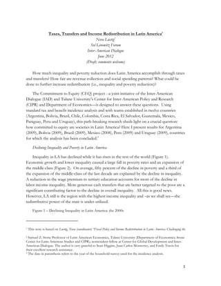
1.
Taxes, Transfers and Income Redistribution in Latin America1
Nora Lustig2
Sol Linowitz Forum
Inter-American Dialogue
June 2012
(Draft; comments welcome)
How much inequality and poverty reduction does Latin America accomplish through taxes
and transfers? How fair are revenue collection and social spending patterns? What could be
done to further increase redistribution (i.e., inequality and poverty reduction)?
The Commitment to Equity (CEQ) project --a joint initiative of the Inter-American
Dialogue (IAD) and Tulane University’s Center for Inter-American Policy and Research
(CIPR) and Department of Economics—is designed to answer these questions. Using
standard tax and benefit incidence analysis and with teams established in twelve countries
(Argentina, Bolivia, Brazil, Chile, Colombia, Costa Rica, El Salvador, Guatemala, Mexico,
Paraguay, Peru and Uruguay), this path-breaking research sheds light on a crucial question:
how committed to equity are societies in Latin America? Here I present results for Argentina
(2009), Bolivia (2009), Brazil (2009), Mexico (2008), Peru (2009) and Uruguay (2009), countries
for which the analysis has been concluded.3
Declining Inequality and Poverty in Latin America
Inequality in LA has declined while it has risen in the rest of the world (Figure 1).
Economic growth and lower inequality caused a large fall in poverty rates and an expansion of
the middle-class (Figure 2). On average, fifty percent of the decline in poverty and a third of
the expansion of the middle-class of the last decade are explained by the decline in inequality.
A reduction in the wage premium to tertiary education accounts for most of the decline in
labor income inequality. More generous cash transfers that are better targeted to the poor are a
significant contributing factor to the decline in overall inequality. All this is good news.
However, LA still is the region with the highest income inequality and –as we shall see—the
redistributive power of the state is under-utilized.
Figure 1 – Declining Inequality in Latin America: the 2000s
1 This note is based on Lustig, Nora (coordinator) “Fiscal Policy and Income Redistribution in Latin America: Challenging the
2 Samuel Z. Stone Professor of Latin American Economics, Tulane University (Department of Economics; Stone
Center for Latin American Studies and CIPR); nonresident fellow at Center for Global Development and Inter-
American Dialogue. The author is very grateful to Sean Higgins, Juan Carlos Monterrey, and Emily Travis for
their excellent research assistance.
3 The date in parenthesis refers to the year of the household survey used for the incidence analysis.
1

2.
2.50
2.02
2.00
1.43
1.50
1.02
Annual Percent Change
1.00
0.51 0.52
0.50 0.21 0.30 0.25
0.00
-0.05
-0.50
-0.60
-1.00 -0.72 -0.66 -0.64
-0.91 -0.90 -0.96
-1.07
-1.50 -1.23 -1.23 -1.22 -1.21 -1.16
-1.47
-2.00
Ecuador
Peru
Venezuela
Mexico
Brazil
Dominican Rep.
Panama
Chile
Uruguay
Honduras
Nicaragua
Total 13
Total 17
India
OECD-30
Bolivia
China
Costa Rica
South Africa
Argentina
El Salvador
Guatemala
Paraguay
Source: López-Calva, Luis F. and Nora Lustig (2010) Declining Inequality in Latin America: a Decade of Progress?,
Brookings Institution and UNDP. The vertical axis shows the yearly decline in the Gini4 coefficient, a standard
indicator used to measure inequality.
Figure 2 – Latin America: Economic Growth, Inequality and Poverty. 1992-2010
2.0
1.5
The 1990s
1.0
0.5
The 2000s
0.0
-0.5
-1.0
Stagnation
-1.5
-2.0
-2.5
-3.0
1992 1993 1994 1995 1996 1997 1998 1999 2000 2001 2002 2003 2004 2005 2006 2007 2008 2009 2010
GDP Poverty Inequality
Source: Gasparini, Leonardo; ppt presentation in Wellbeing and inequality in the long run: measurement, history and ideas,
Madrid, May 31, 2012. Poverty is the headcount ratio using the US$4 a day in purchasing power parity poverty
line. Unweighted averages.
How Much Redistribution through Income Taxes and Cash Transfers?
The reduction in income inequality and poverty from income taxes and direct cash
transfers varies greatly across countries (Figure 3). In our sample, Argentina and Brazil are
4A standard measure of income inequality, the Gini coefficient ranges between 0 (perfect equality) and 1 (fully
unequal) (or 100 if expressed in percent).
2

3.
the most redistributive while Peru is the least. Uruguay reduces poverty the most and, again,
Peru the least. Although governments have become more redistributive in LA, the extent of
inequality and poverty reduction attained through taxes and transfers is still far lower than in
rich OECD countries. On average, taxes and transfers reduce inequality seven times more in
the latter (measured by the reduction in Gini points, a standard measure of inequality). When
making these comparisons, however, one should be careful not to jump to sweeping
conclusions. Some of the differences might be due to higher living standards, demographics,
geography and institutional factors prevailing in rich OECD countries, and not just to
differences in commitment to equity.
Figure 3 – Decline in Inequality and Poverty due to Direct Taxes and Transfers
Decline in Inequality (Gini coefficient; in %)
0.0%
Argen2na% Brazil% Uruguay% Bolivia% Mexico% Peru%
!1.0%
!2.0%
!3.0%
!4.0%
!5.0%
!6.0%
!7.0%
!8.0%
Decline in Poverty (Headcount Ratio with US$2.50 a day poverty line; in %)
0.0&
Uruguay& Argen3na& Brazil& Mexico& Bolivia& Peru&
!5.0&
!10.0&
!15.0&
!20.0&
!25.0&
!30.0&
!35.0&
!40.0&
!45.0&
Source: Lustig, coordinator (2012). See first footnote for full citation.
Interestingly, the governments’ capacity to spend or “fiscal space” (measured by the ratio
of primary spending5 to total output or GDP) and the extent of redistribution are not
correlated. Countries with more fiscal space, higher social spending (as a share of total output),
or that spend more on direct cash transfers, are not necessarily more redistributive (Figure 4).
5 Primary spending excludes debt servicing. For details see Lustig et al. (2012).
3

4.
For example, Argentina and Bolivia have an equally large capacity to spend but these two
countries are on opposite sides in terms of the extent of inequality reduction. Uruguay’s
capacity to spend is considerably lower than that of Bolivia, yet both inequality and poverty
reduction are higher in the former. Brazil spends the most on direct cash transfers as a
proportion of GDP, yet it achieves much less poverty reduction than Uruguay, which allocates
much less to cash transfers. Bolivia spends on direct transfers substantially more than Mexico
but the latter reduces poverty by an almost the same proportion.
Figure 4 - Government Spending and Decline in Inequality and Extreme Poverty
Large governments do not necessarily lower inequality by more…
10.0% 50.00%
8.0% 40.00%
6.0% 30.00%
4.0% 20.00%
%%change%wrt%net%market%
2.0% 10.00% income%
0.0% 0.00% Primary%spending%as%a%%%of%
GDP%
%
il%
a%
%
%
y%
na
ico
ru
!2.0% !10.00%
az
ivi
ua
Pe
n1
ex
Br
l
ug
Bo
ge
M
Ur
!4.0% !20.00%
Ar
!6.0% !30.00%
!8.0% !40.00%
Large governments do not necessarily lower extreme poverty by more…
45.0&
35.0&
25.0&
15.0&
5.0& Primary&spending&as&a&%&of&
!5.0& GDP&
&
il&
&
a&
&
y&
na
ico
ru
az
ivi
ua
Pe
n3
ex
Br
l
ug
!15.0&
Bo
ge
M
Ur
Ar
!25.0&
!35.0&
!45.0&
Source: Lustig, coordinator (2012). Percentage change in Gini coefficient and headcount
ratio for the US$2.50 a day poverty line. Primary spending excludes debt servicing.
Direct Cash Transfers and Poverty Reduction
Our results suggest that merely increasing the overall spending capacity of the state or the
capacity to spend on direct cash transfers will not necessarily reduce extreme poverty by as
4

5.
much as one might expect.6 In order for direct transfers to make a noticeable dent on extreme
poverty, two things must happen. First, cash transfer programs (also called safety nets) must
cover a very high proportion of the extreme poor. That is, the existing range of safety net
programs must be designed and implemented in such a way as to cover as close to the universe
of the extreme poor as possible (both in normal times and in the face of adverse shocks).
Second, spending on direct cash transfers and the proportion of benefits to the extreme poor
must be large enough so that transfers per beneficiary are not too distant from the average
poverty gap (i.e., the difference between the poverty line and the per poor person income).
6 Extreme poverty is defined using the international poverty line of US$2.50 per day in purchasing power parity.
5

6.
Figure 5 – Distribution of Benefits/Beneficiaries of Cash Transfers and Coverage among the
Poor
Percent'of'Benefits'Going'to…
'Percent'of'Beneficiaries'who'are…
Percent'of'Poor'who'are'Beneficiaries
Source: Lustig, coordinator (2012). For full citation see first footnote.
Of the six countries considered, Argentina and Uruguay achieve the largest reductions in
extreme poverty per amount spent on cash transfers. Mexico and Peru have well-targeted
programs but the amount these countries spend on direct cash transfers is too small and the
range of safety net programs--by design--exclude around thirty and forty percent of the
extreme poor, respectively (Figure 5); the flagship anti-poverty programs (Oportunidades in
Mexico and Juntos in Peru) in these two countries exclude--or are unable to reach--the urban
extreme poor. Interestingly, although Brazil spends the most on direct cash transfers of all six
countries (4.2 percent of GDP), the extent of poverty reduction is smaller than in, for
6

7.
example, Argentina because the share of transfers going to the poor is smaller in Brazil: 10
percent versus 36 percent in Argentina. In Brazil, the largest cash transfer—the Special
Circumstances Pension—is not a program targeted to the poor.
Although Argentina and Mexico are similar in terms of per capita GDP (measured in
purchasing power parity the latter was around 14,000 dollars per year), Argentina spends more
on cash transfers (3.0 percent versus .75 percent of GDP) and a larger percentage of the
extreme poor are transfer beneficiaries in Argentina than in Mexico (92.5 versus 66.8 %)
(Figure 5). Unsurprisingly, transfers in Argentina reduce extreme poverty by a considerably
larger amount. This is true, however, in the short-run. Since the pension moratorium program
may incentivise informality, the formal social security system could face sustainability issues in
the future. Also, public revenues in Argentina have been particularly high due to the
commodity boom. The government may be unable to support generous cash transfers under
more adverse conditions.
Bolivia spends almost three times as much as Mexico on transfers as a share of GDP, but
because Bolivia’s GDP is lower, the transfers per beneficiary are smaller than in Mexico.
However, what makes Bolivia’s redistributive machine less effective is that more than 60
percent of the benefits of its largest transfer programme —Renta Dignidad, a non-contributory
universal pension (1.4 percent of GDP)—go to the non-poor. Meanwhile, only 43 percent of
the extreme poor are beneficiaries of any of Bolivia’s flagship transfer programmes. Bolivia’s
emphasis on universal direct cash transfers (as opposed to targeted ones) substantially
diminishes its capacity to reduce extreme poverty (through cash transfers).
In sum, Argentina has to address issues related to fiscal sustainability and distortions
introduced by its safety net programs. Bolivia must make its safety net programs considerably
better targeted to the poor or increase spending on these programs substantiatially. Mexico,
Peru and to a lesser extent Uruguay must increase the amount spent on direct cash transfers.
Brazil, Mexico and Peru and above all Bolivia should adapt or expand the range of safety net
programs to cover a larger share of the extreme poor. (Brazil has already started addressing the
limitations of its anti-poverty programs (including those of Bolsa Familia) with the recent
launch of Brasil Carinhoso).
Who Bears the Burden of Taxes?
Income taxes are progressive: that is, the proportion paid in income tax rises with income
in Argentina, Brazil, Mexico, Peru and Uruguay. However, one cannot really assess the
progressivity of income taxes without having access to the information reported in tax returns.
It is about time that LA governments make the information from tax returns public the same
way that all OECD-member countries--except for Chile, Mexico and Turkey--do (and have
been doing it for decades). In addition, from public accounts one knows that personal
7

8.
income taxes represent a small proportion of total tax revenues. Bolivia doesn’t even have
income taxes. Any tax reform in the future should seriously examine the redistributive
potential coming from higher income (and wealth) taxes on the rich. Again, this will require
revealing the current effective tax rates at the very top.
In Figure 6, I show the share of market (before taxes and transfers) income and the share
of indirect taxes by decile. Indirect taxes (mostly VATs) are clearly regressive: that is, the poor
pay a higher proportion of their income in indirect taxes and the proportion declines with
income. Perhaps more importantly, once we take into account the impact of indirect taxes on
incomes, people in the second, third and fourth deciles (depending on the country) become
net payers to the government (Figure 7). Furthermore, indirect taxes can make the poor worse
off in a nontrivial way. For example, in Brazil--even after all the benefits from cash transfers
are taken into account—due to indirect taxes around 20 percent of the moderate poor become
extreme poor and, on average, their income declines by 10 percent.
Figure 6 - Distribution of market income (red) and indirect taxes (blue) by decile
Argentina Bolivia
40.0%$ 40.0%$
35.0%$ 35.0%$
Concentra)on*Share*
Concentra)on*Share*
30.0%$ 30.0%$
25.0%$ 25.0%$
20.0%$ 20.0%$
15.0%$ 15.0%$
10.0%$ 10.0%$
5.0%$ 5.0%$
0.0%$ 0.0%$
1$ 2$ 3$ 4$ 5$ 6$ 7$ 8$ 9$ 10$ 1$ 2$ 3$ 4$ 5$ 6$ 7$ 8$ 9$ 10$
Decile* Decile*
Brazil Mexico
50.0%$ 45.0%$
45.0%$ 40.0%$
40.0%$ 35.0%$
Concentra)on*Share*
Concentra)on*Share*
35.0%$ 30.0%$
30.0%$
25.0%$
25.0%$
20.0%$
20.0%$
15.0%$ 15.0%$
10.0%$ 10.0%$
5.0%$ 5.0%$
0.0%$ 0.0%$
1$ 2$ 3$ 4$ 5$ 6$ 7$ 8$ 9$ 10$ 1$ 2$ 3$ 4$ 5$ 6$ 7$ 8$ 9$ 10$
Decile* Decile*
Source: Lustig, coordinator (2012). See first footnote for full citation.
8

9.
Figure 7 – Change in Income by Decile After Cash Transfers and Direct and Indirect Taxes
Source: Lustig, coordinator (2012). See first footnote for full citation.
The regressive and poverty-increasing effect of indirect taxes poses a serious challenge.
Indirect taxes—VAT in particular—are known to be one of the most efficient and effective
revenue-raising mechanisms. Governments will need to decide whether to offset the negative
impact of indirect taxes on inequality and poverty through exemptions (on food consumed in
large quantities by the poor, for example) or higher and more comprehensive direct cash
transfers.
How much gets redistributed through public spending in education and health?
Governments redistribute and improve living standards not just with cash transfers but
also through the provision of free (or almost free) government services especially in the areas
of education and health. When we impute the “value” of those transfers to the households
that use public education and health services, the extent of redistribution rises by a significant
amount. In Figure 8 we trace the “evolution” of the Gini coefficient through its fiscal path.
The disposable income Gini equals the market Gini minus income taxes plus cash transfers.
The post-fiscal Gini equals the disposable income Gini minus indirect taxes. The final income
Gini equals the post-fiscal Gini plus the “income” transferred in the form of public education
and health. As one can observe, the largest decline in inequality is due to the in-kind transfers
in education and health.
9

10.
Figure 8 – Taxes, Transfers and Inequality (Gini Coefficient)
Source: Lustig, coordinator (2012). See first footnote for full citation. For definitions of income
concepts see text.
In all six countries analyzed here, spending on education and health is progressive: that is,
the post-transfers inequality levels are lower than market income inequality. In fact, in several
countries, education and health spending is progressive in absolute terms: that is, the per capita
benefits decline with income. This can be observed in Figure 9. Any time the share of
spending on the bottom two deciles exceeds ten percent, spending is progressive in absolute
terms.
Redistribution through social spending on education and health is quite significant in LA.
The main problem is not access but the low quality of these services, in particular for the poor.
Thus, even though access to education and health services is quite equitable in the region,
opportunities are not equalized. Low quality education and health condemn poor children to
limited earning-power in the future. And today’s inequality in the quality of education might
bring the auspicious declining inequality momentum of the last decade to an end.
10

11.
Figure 9 – Distribution of Market Income and Distribution of Public Spending on
Education and Health (by decile)
Public'Education Public'Health
Argentina
40.0%' 40.0%$
35.0%'
Concentra)on*Share*
35.0%$
30.0%'
Concentra)on*Share*
30.0%$
25.0%' 25.0%$
20.0%' 20.0%$
15.0%' 15.0%$
10.0%'
10.0%$
5.0%'
5.0%$
0.0%'
1' 2' 3' 4' 5' 6' 7' 8' 9' 10' 0.0%$
1$ 2$ 3$ 4$ 5$ 6$ 7$ 8$ 9$ 10$
Decile* Decile*
Bolivia
40.0%' 40.0%'
Concentra)on*Share*
Concentra)on*Share*
35.0%'
30.0%' 30.0%'
25.0%'
20.0%' 20.0%'
15.0%'
10.0%' 10.0%'
5.0%'
0.0%' 0.0%'
1' 2' 3' 4' 5' 6' 7' 8' 9' 10' 1' 2' 3' 4' 5' 6' 7' 8' 9' 10'
Decile* Decile*
Brazil
50.0%' 50.0%'
Concentra)on*Share*
Concentra)on*Share*
40.0%' 40.0%'
30.0%' 30.0%'
20.0%' 20.0%'
10.0%' 10.0%'
0.0%' 0.0%'
1' 2' 3' 4' 5' 6' 7' 8' 9' 10' 1' 2' 3' 4' 5' 6' 7' 8' 9' 10'
Decile* Decile*
11

12.
Figure 9 (continued)
Public'Education Public'Health
Mexico
50.0%' 50.0%'
Concentra)on*Share*
Concentra)on*Share*
40.0%' 40.0%'
30.0%' 30.0%'
20.0%' 20.0%'
10.0%' 10.0%'
0.0%' 0.0%'
1' 2' 3' 4' 5' 6' 7' 8' 9' 10' 1' 2' 3' 4' 5' 6' 7' 8' 9' 10'
Decile* Decile*
Peru
45.0%' 45.0%'
40.0%' 40.0%'
Concentra)on*Share*
Concentra)on*Share*
35.0%' 35.0%'
30.0%' 30.0%'
25.0%' 25.0%'
20.0%' 20.0%'
15.0%' 15.0%'
10.0%' 10.0%'
5.0%' 5.0%'
0.0%' 0.0%'
1' 2' 3' 4' 5' 6' 7' 8' 9' 10' 1' 2' 3' 4' 5' 6' 7' 8' 9' 10'
Decile* Decile*
Uruguay
Source: Lustig, coordinator (2012). See first footnote for full citation.
12