Creating Pivot Table in Excel.

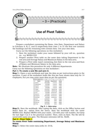
1. Use of Pivot Tables (Practical) 317
Prepare a worksheet containing the Name, Join Date, Department and Salary
in Columns A, B, C, and D respectively from rows 1 to 31 the first row contains
the headings and the remaining rows contain data. Use your own data.
Carry out the following operations on this worksheet.
1. Save the worksheet under your name followed by your roll no., question
no. e.g. MONA1232
2. Prepare another Pivot table on the same data taking Department in the
row area and Average Salary and Maximum Salary in the data area.
3. Prepare a Pivot table report containing Join Date in the row area and Sum
of Salary and Minimum Salary in the data area.
Note : We illustrate this procedure for only 4 different departments.
Carry out the following operations on this worksheet :
Part 1: To create a new file and save it.
Step 1 : Open a new workbook and type the data as per instructions given in the
question. A part of the worksheet looks like this (we have shown data only for 14
employees, but you may enter more data as per the question).
Fig. P. 1 : Data entry
Step 2 : Save the workbook: After typing the data, click on the Office button and
Select Save As.. option from the menu. Save the workbook with the name
MONA1233. Replace MONA with your name, 123 with your roll number, but keep
the last digit 3 as it is the practical number. Then, click on Save. The file will be
saved with name you gave. The filename extension will be. XLSX.
Part 2 : Pivot Table 1
To create Pivot Table containing Department, Average Salary and Maximum
Salary.
Step 1 : Select the entire data (cells A1: D15).
Use of Pivot Tables
III – 3 – (Practicals)

2. 318 Computer Systems & Applications (T. Y. B. Com. – Sem. – VI) – Mukesh N Tekwani
Step 2 : From the Insert menu. Click on the Pivot Table button and then select
sub-option Pivot table. The Pivot Table button is shown below :
Step 3 : The Pivot Tables dialog box appears as shown below. Accept the selected
range A1:D19. Click on “New Worksheet”.
Fig. P. 2 : Pivot Table Dialog Box – Range and Location
The data that we highlighted is in the Table/Range text box. This is selected
automatically. We select the New Worksheet as the location for the pivot table.
Click OK.
Excel shows the following window on the right of the screen :
Fig. P. 3 : Pivot Table – Field List
Step 4 : In Pivot Table field list, click on Department and drag it to the Row area.
Location
Selected
automatically

3. Use of Pivot Tables (Practical) 319
Step 5 : In Pivot Table filed list, click on the Salary field and drag it to the Value
area. It is displayed as ‘Sum of salary’. Click on it and select value field settings
(Fig. P. 4).
Fig. P. 4 : Value Field Settings Fig. P. 5 : Value Field Settings – Selecting Min
Step 6 : Select the type of calculation as ‘Min’ and click on ‘ok’ to obtain Min of
Salary(Fig P. 5).
Step 7 : Again Drag the ‘Salary’ to value area. It is displayed as ‘Sum of salary’.
Fig. P. 6 : Pivot Table – Field List after Step 6

4. 320 Computer Systems & Applications (T. Y. B. Com. – Sem. – VI) – Mukesh N Tekwani
The completed Pivot table is displayed on the left in the worksheet. This Pivot
table is shown below :
Fig. P. 7 : The completed Pivot Table
Conclusion : From this pivot table, we can draw the following conclusions:
a) The minimum salary of each department is indicated against the
department name.
b) The total salary for each department is indicated against the department
name.
Part 3 : Pivot Table 2
To create Pivot Table containing Joining Date, Sum of Salary and Minimum
salary
Step 1 : Select the entire data (cells A1: D15).
Step 2 : From the Insert menu. Click on the Pivot Table button and then select
sub-option Pivot table.
Step 3 : The Pivot Tables dialog box appears as shown below. Accept the selected
range A1:D15. Click on “Existing Worksheet” and type location as A50.
Excel shows the following window on the left and right of the screen :
Fig. P. 8 : Pivot Table place holder Fig. P. 9 : Pivot Table: Field List

5. Use of Pivot Tables (Practical) 321
Step 4 : In Pivot Table field list, click on join Date and drag it to the Row area.
Step 5 : In Pivot Table field list, click on the Salary field and drag it to the Value
area. It is displayed as ‘Sum of salary’. Click on it and select value field settings.
Step 6 : Select the type of calculation as ‘Min’ and click on ‘ok’ to obtain Min of
Salary.
Step 7 : Again Drag the ‘Salary’ to value area. It is displayed as ‘Sum of salary’.
The field list is shown in Fig. P. 10 below :
Fig. P. 10 : Field List
The completed Pivot table is displayed on the left in the worksheet. This Pivot
table is shown below :
Fig. P. 11 : Completed Pivot Table
Optional Note
In the above table we see that row 58 contains the Grand Total. This contains
the minimum salary of all those shown above (25000). Similarly, the sum of all
salaries is shown as 456800. If this row is not required, we can remove it by
selecting the Pivot Table and modifying its properties.

6. 322 Computer Systems & Applications (T. Y. B. Com. – Sem. – VI) – Mukesh N Tekwani
Selecting Pivot Table and Modifying its properties
Step 1 : Click on cell A50 since that is the location of the Pivot Table.
Step 2 : Right click and select PivotTable options. It brings up the following
dialog box (Fig. P. 12).
Fig. P. 12 : Pivot Table Options Dialog Box
Step 3 : Select the Totals & Filters tab (shown below in Fig. P. 13).
Fig. P. 13 : Pivot Table Options Dialog Box – Totals & Filters
Deselect this check
box
Select this tab

7. Use of Pivot Tables (Practical) 323
Deselect the option “Show grand totals for columns” and click OK. The Pivot
table now changes to the following :
Fig. P. 14 : Final Pivot Table, without column totals