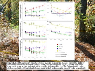
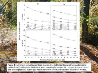
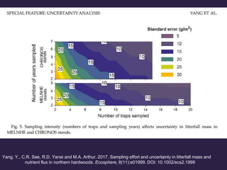
Sampling intensity affects the ability to detect changes over time in soil nutrient concentrations. Higher sampling intensity through more samples or sampling sites allows for detection of smaller minimum detectable differences. A study analyzed how sampling intensity over time and space impacted the minimum detectable annual percentage change for concentrations of total carbon, nitrogen, and exchangeable magnesium, calcium, and potassium at different soil depths. The results provide guidance on sampling designs to balance detecting desired changes against costs of sample collection and analysis for soil monitoring.


![Polymer [ बहुलक ] Chemistry Notes PDF - Irfanullah Mehar - JJ Sir Chemistry.pdf](https://cdn.slidesharecdn.com/ss_thumbnails/polymerchemistrynotespdf-irfanullahmehar-jjsirchemistry-260210172118-3f9b37f7-thumbnail.jpg?width=640&height=640&fit=bounds)


