Copying Files Across Workbooks Lab 5, Step 1 A. Save all of the wk5_Chap7_cap iLab files to one folder. You should have the following files: B. Open the Summary workbook in Excel. C. Open one of the files you wish to consolidate into this workbook. From the Home tab, the Cells group, the Format option, select Move or Copy Sheet. From the Move or Copy dialog box, select the Summary worksheet as location, Move to End, and Create a Copy: Click OK. Copy the Eastside and Westside data in the same way. Your worksheet will now look like this: Save this consolidated file as Lab5_yourlastname.xlsx. Note: Use the Switch Windows command from the View tab to see what is open, and use the Close button to close all worksheets except the Lab 5 Summary worksheet. Your Lab 5 Summary worksheet should now look like this: Creating a Scenario Summary Lab 6, Step 4 A. Name the cells that will be used in the Scenario Summary. To use the labels you have already created in the Income Statement, select the two columns from the Income Statement in the Assumptions area: In the Formula tab in the Defined Names Group, select “Create from Selection”. Select the Left column as your name: Click OK. When you click on the right hand cell, notice that the cell is now named: Repeat the process and name all of the cells in your Income Statement as you did in the steps above: • Tuition per Day • Food Expenses • Supplies per Year • Teacher Cost • Insurance • Maintenance • Administrative & Advertising • Est. Taxes • Total Revenue • Total Expenses • Net Income (Make sure to also label the net income) B. Define Scenarios From the Data tab, click What-If Analysis, and then select Scenario Manager: The Scenario Manager Dialog Box opens. Click Add to begin defining your scenarios. Provide a name in the first textbox: Now select the cells that will change. You can select multiple cells by holding down the Control (Ctrl) key as you make your selections. Or you may type a comma after you select each variable. Select Number of Children (B6), Teacher Cost (B8), Supplies (B10), and Tuition (B13): Click OK. Add the values for your first scenario: Click OK. Add your second scenario with the same Changing Cells: Click OK and then add the Changing Values: Click OK and then add your final scenario. Name it High and add the values: To test your scenario, click Show. Your Income Statement will now contain the values you specified: Click Close to exit the Scenario Manager. Change your values back to the original assumptions: C. Create a Scenario Summary to display the scenarios you have created. Go back to the Data tab, click What-If Analysis, and then select Scenario Manager: Click Summary in the Scenario dialog box.

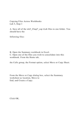
1. Copying Files Across Workbooks
Lab 5, Step 1
A. Save all of the wk5_Chap7_cap iLab files to one folder. You
should have the
following files:
B. Open the Summary workbook in Excel.
C. Open one of the files you wish to consolidate into this
workbook. From the Home tab,
the Cells group, the Format option, select Move or Copy Sheet.
From the Move or Copy dialog box, select the Summary
worksheet as location, Move to
End, and Create a Copy:
Click OK.

2. Copy the Eastside and Westside data in the same way. Your
worksheet will now look like
this:
Save this consolidated file as Lab5_yourlastname.xlsx.
Note: Use the Switch Windows command from the View tab to
see what is open, and use
the Close button to close all worksheets except the Lab 5
Summary worksheet.
Your Lab 5 Summary worksheet should now look like this:
Creating a Scenario Summary
Lab 6, Step 4
A. Name the cells that will be used in the Scenario Summary.

3. To use the labels you have already created in the Income
Statement, select the two
columns from the Income Statement in the Assumptions area:
In the Formula tab in the Defined Names Group, select “Create
from Selection”. Select
the Left column as your name:
Click OK. When you click on the right hand cell, notice that
the cell is now named:
Repeat the process and name all of the cells in your Income
Statement as you did in the
steps above:
• Tuition per Day
• Food Expenses
• Supplies per Year
• Teacher Cost
• Insurance
• Maintenance
• Administrative & Advertising
• Est. Taxes

4. • Total Revenue
• Total Expenses
• Net Income (Make sure to also label the net income)
B. Define Scenarios
From the Data tab, click What-If Analysis, and then select
Scenario Manager:
The Scenario Manager Dialog Box opens.
Click Add to begin defining your scenarios.
Provide a name in the first textbox:
Now select the cells that will change. You can select multiple
cells by holding down the
Control (Ctrl) key as you make your selections. Or you may
type a comma after you
select each variable.

5. Select Number of Children (B6), Teacher Cost (B8), Supplies
(B10), and Tuition (B13):
Click OK.
Add the values for your first scenario:
Click OK.
Add your second scenario with the same Changing Cells:
Click OK and then add the Changing Values:
Click OK and then add your final scenario. Name it High and
add the values:

6. To test your scenario, click Show. Your Income Statement will
now contain the values
you specified:
Click Close to exit the Scenario Manager.
Change your values back to the original assumptions:
C. Create a Scenario Summary to display the scenarios you
have created. Go back to
the Data tab, click What-If Analysis, and then select Scenario
Manager:
Click Summary in the Scenario dialog box:

7. Select Scenario Summary and then choose the Result Cells:
Total Revenue (B31), Total
Expenses (B32), Net Income (B33):
Click OK.
Your Scenario Summary will be created on a new sheet:
D. Move this sheet to the end of the workbook.
Creating a Two-Variable Data Table
Lab 6, Step 3
A. Set up your Two-Variable Data Table
Create headings that describe the data table. Your columns
(row input cells) will be
labeled 6 through 15 (number of children):
You can copy and paste the row headings from your one-
variable data table.

8. Create row labels (column input cells) that range from 35 – 75
in $5 increments:
B. Create your Results cell in the upper left corner of the data
table. This cell will
reference your Net Income (B33).
Change the Format of this cell to read Fees. Right-click on the
Result Cell, select
Format Cells. In the Format Cells dialog box, click the Number
tab, select Custom,
and then type in “Fees” with quotes into the Type textbox.
Click OK.
C. Add a heading that explains the data table and shading to
match the shading of the
original Income Statement:
D. Select all of the cells that hold the data table area (without

9. the descriptive heading).
Create your data table using the Data tab, What-If Analysis,
Data Table option.
Reference the cell that contains the number of children as the
Row Input (B6) and Fee
as the Column Input (B13):
Click OK. The data table will be populated with values:
Format the results as currency with no decimals. Apply
conditional formatting to show
all options that are above Jane’s target goal.
Your data table should now look something like this:
Select the
area that
includes
all of the
variable
labels

10. Creating a One-Variable Data Table
Lab 6, Step 2
A. Set up your One-Variable Data Table
Create headings that describe the data table. Your columns will
be labeled Initial Values
and then 6 through 15 (number of children) and your rows will
be labeled Expenses and
Net Income:
Add a heading that explains the data table and shading to match
the shading of the
original Income Statement:
B. Reference the cells that hold the Result Values you wish to
use. These references
will be added to the Initial Values area. Reference the cell that
contains Total
Expenses (=B32) and the cell that contains Net Income (=B33) :
C. Select the data table area except the descriptive labels.
From the Data tab, under
What-If Analysis Tools, select Data Table:

11. The Data Table dialog box will appear. Select the cell that
holds the variable you wish to
change. Since the variable is in the first row, enter this in the
Row Input Cell area:
Click OK. The data table will be populated with values:
Format the results as currency with no decimals:
D. Apply conditional formatting to show all options that are
above Jane’s target goal:
Creating 3D Cell References and Using Worksheet Grouping
Lab 5, Step 2

12. Make sure that the Lab 5 Summary file is open in Excel.
A. Fill in the first formula required using 3D cell reference to
refer to data on multiple
worksheets.
Select Cell B3 on the Summary worksheet and type =SUM(
Click the Westside tab to begin the 3D cell referencing. Hold
down the Shift key and
select the last worksheet, for example, Downtown. Click in
Cell B3. Press the Enter key
to add an ending parenthesis and complete the formula. You
will see the results of the
formula in Cell B3.
Click on Cell B3 to review the formula Excel has created:
Note that this cell reference tells Excel to total the contents in
Cell B3 for all worksheets
from Westside through Downtown.
B. You can copy this formula across and then down to see the
sales by quarter for each

13. of the dining categories:
C. Use Grouping to add Totals to all worksheets:
Select all worksheets by clicking on the first and last worksheet
tabs while holding down
the Shift key. The tabs will become white:
The filename will also show that the worksheets are Grouped:
Select Cell B6 and create the formula to total results of Cells
B3 through B5:
Hit the Enter key. Notice that this formula has been applied to
all sheets in the
workbook:

14. Make sure the Worksheets are grouped. Drag the formula
across the row:
Create the formula for the Grand Total while the sheets are
grouped and then drag this
formula to copy it in the Grand Total row:
Ungroup the worksheets. Verify that the formula has been
copied to all worksheets.