1. MTRN9224 Robot Design
Lecture 1: Introduction
Tomonari Furukawa
School of Mechanical and Manufacturing Engineering
University of New South Wales
1 HISTORY
19th
century – Industrial Revolution (Birth of Mechanical Engineering)
Mines needed large pumps never before seen to keep their shafts dry
Iron and steel mills required pressures and temperatures beyond levels used
commercially until then
Transportation systems needed more than real horse power to move goods
Structures began to stretch across ever wider abysses and to climb to dizzying heights
Manufacturing moved from the shop bench to large factories
↓
Engineering disciplines
People began to specialize and build bodies of knowledge.
Early 20th
century – Growth of individual engineering disciplines
Each discipline (body of
knowledge) has grown
individually
Mechanical engineering
Electrical engineering
Civil engineering
Chemical engineering
2
Mid 20th
century – Divergence of individual engineering disciplines
Mechanical engineering
Aeronautical engineering
Space engineering
Naval engineering
Precision engineering
Manufacturing, etc
Mechanical engineering
Electrical engineering
Civil engineering
Chemical engineering
Electrical engineering
Electronical engineering, etc
Civil engineering
Structural engineering, etc
Chemical engineering
Biochemical engineering, etc
Late 20th
century – Information revolution (Semiconductor and information technologies)
Mechanical engineering
Aeronautical engineering
Space engineering
Naval engineering
Precision engineering
Manufacturing, etc
Electrical engineering
Electronical engineering, etc
Civil engineering
Structural engineering, etc
Chemical engineering
Biochemical engineering, etc
Semiconductor technology
Information technology
CuuDuongThanCong.com https://fb.com/tailieudientucntt
c
u
u
d
u
o
n
g
t
h
a
n
c
o
n
g
.
c
o
m
2. 3
2 MECHATRONICS
2.1 Difinition
Interdisciplinary field or engineering dealing with the design of products whose function relies on
the integration of mechanical and electronic components coordinated by a control architecture.
Originally introduced in Japan in early 1960’s, spread in Europe in late 1960’s and then in USA
in early 1970’s.
Primary disciplines – Mechanics, electronics, controls and computer engineering
Examples of Mechatronics systems
Aercraft flight control and navigation system
Automobile electronic fuel injection and antilock brake systems
Numerically controlled (NC) machine tools
Robots
Smart kitchen
Toys, etc
Figure 1.1 illustrates all the components in a typical mechatronic system.
Actuators – produce motion or cause some action
Sensors – detect the state of the system parameters, inputs and outputs
Digital devices – control the system
Conditioning and interfacing circuits – provide connections between the control
circuits and the input/output devices
Graphical displays – provide visual feedback to users
4
3 ROBOTS
3.1 Difinition
A reprogrammable, multifunctional manipulator designed to move material, parts, tools, or
specialized devices through various programmed motions for the performance of a variety of tasks.
A more inspiring definition can be found in Webster. According to Webster a robot is:
An automatic device that performs functions normally ascribed to humans or a machine in the
form of a human.
3.2 History
First use of the word 'robot'
The acclaimed Czech playwright Karel Capek (1890-1938) made the first use of the word ‘robot’,
from the Czech word for forced labor or serf. Capek was reportedly several times a candidate for the
Nobel prize for his works and very influential and prolific as a writer and playwright.
The use of the word Robot was introduced into his play R.U.R. (Rossum's Universal Robots) which
opened in Prague in January 1921.
In R.U.R., Capek poses a paradise, where the machines initially bring so many benefits but in the
end bring an equal amount of blight in the form of unemployment and social unrest.
The play was an enormous success and productions soon opened throughout Europe and the U.S.
R.U.R's theme, in part, was the dehumanization of man in a technological civilization.
You may find it surprising that the robots were not mechanical in nature but were created through chemical means. In
fact, in an essay written in 1935, Capek strongly fought that this idea was at all possible and, writing in the third person,
said:
"It is with horror, frankly, that he rejects all responsibility for the idea that metal contraptions could ever replace human
beings, and that by means of wires they could awaken something like life, love, or rebellion. He would deem this dark
prospect to be either an overestimation of machines, or a grave offence against life."
[The Author of Robots Defends Himself - Karl Capek, Lidove noviny, June 9, 1935, translation: Bean Comrada]
There is some evidence that the word robot was actually coined by Karl's brother Josef, a writer in his own right. In a
short letter, Capek writes that he asked Josef what he should call the artificial workers in his new play.
Karel suggests Labori, which he thinks too 'bookish' and his brother mutters "then call them Robots" and turns back to
his work, and so from a curt response we have the word robot.
CuuDuongThanCong.com https://fb.com/tailieudientucntt
c
u
u
d
u
o
n
g
t
h
a
n
c
o
n
g
.
c
o
m
3. 5
First use of the word 'robotics'
The word 'robotics' was first used in Runaround, a short story published in 1942, by Isaac
Asimov (born Jan. 2, 1920, died Apr. 6, 1992). I, Robot, a collection of several of these stories,
was published in 1950.
One of the first robots Asimov wrote about was a robotherapist. A modern counterpart to
Asimov's fictional character is Eliza. Eliza was born in 1966 by a Massachusetts Institute of
Technology Professor Joseph Weizenbaum who wrote Eliza -- a computer program for the
study of natural language communication between man and machine.
She was initially programmed with 240 lines of code to simulate a psychotherapist by
answering questions with questions.
Three Laws of Robotics
Asimov also proposed his three "Laws of Robotics", and he later added a 'zeroth law'.
Law Zero: A robot may not injure humanity, or, through inaction, allow humanity to come to harm.
Law One: A robot may not injure a human being, or, through inaction, allow a human being to come to harm, unless this
would violate a higher order law.
Law Two: A robot must obey orders given it by human beings, except where such orders would conflict with a higher
order law.
Law Three: A robot must protect its own existence as long as such protection does not conflict with a higher order law.
The First Robot: 'Unimate'
After the technology explosion during World War II, in 1956, a historic meeting
occurs between George C. Devol, a successful inventor and entrepreneur, and
engineer Joseph F. Engelberger, over cocktails the two discuss the writings of
Isaac Asimov.
Together they made a serious and commercially successful effort to develop a
real, working robot. They persuaded Norman Schafler of Condec Corporation in
Danbury that they had the basis of a commercial success.
Engelberger started a manufacturing company 'Unimation' which stood for
universal automation and so the first commercial company to make robots was
formed. Devol wrote the necessary patents. Their first robot nicknamed the
'Unimate'. As a result, Engelberger has been called the 'father of robotics.'
The first Unimate was installed at a General Motors plant to work with heated
die-casting machines. In fact most Unimates were sold to extract die castings
from die casting machines and to perform spot welding on auto bodies, both
tasks being particularly hateful jobs for people.
Both applications were commercially successful, i.e., the robots worked reliably and saved money by replacing people.
An industry was spawned and a variety of other tasks were also performed by robots, such as loading and unloading
machine tools.
Ultimately Westinghouse acquired Unimation and the entrepreneurs' dream of wealth was achieved. Unimation is still in
production today, with robots for sale.
The robot idea was hyped to the skies and became high fashion in the Boardroom. Presidents of large corporations
bought them, for about $100,000 each, just to put into laboratories to "see what they could do;" in fact these sales
constituted a large part of the robot market. Some companies even reduced their ROI (Return On Investment criteria for
investment) for robots to encourage their use.
6
Modern Industrial Robots
The image of the "electronic brain" as the principal part of the robot
was pervasive. Computer scientists were put in charge of robot
departments of robot customers and of factories of robot makers.
Many of these people knew little about machinery or manufacturing
but assumed that they did.
(There is a common delusion of electrical engineers that mechanical
phenomena are simple because they are visible. Variable friction, the
effects of burrs, minimum and redundant constraints, nonlinearities,
variations in workpieces, accommodation to hostile environments and
hostile people, etc. are like the "Purloined Letter" in Poe's story, right
in front of the eye, yet unseen.) They also had little training in the
industrial engineer's realm of material handling, manufacturing
processes, manufacturing economics and human behavior in
factories.
As a result, many of the experimental tasks in those laboratories were made to fit their robot's capabilities but had little to
do with the real tasks of the factory.
Modern industrial arms have increased in capability and performance through controller and language development,
improved mechanisms, sensing, and drive systems. In the early to mid 80's the robot industry grew very fast primarily
due to large investments by the automotive industry.
The quick leap into the factory of the future turned into a plunge when the integration and economic viability of these
efforts proved disastrous. The robot industry has only recently recovered to mid-80's revenue levels.
In the meantime there has been an enormous shakeout in the robot industry. In the US, for example, only one US
company, Adept, remains in the production industrial robot arm business. Most of the rest went under, consolidated, or
were sold to European and Japanese companies.
In the research community the first automata were probably Grey Walter's machina (1940's) and the John's Hopkins
beast. Teleoperated or remote controlled devices had been built even earlier with at least the first radio controlled
vehicles built by Nikola Tesla in the 1890's.
Tesla is better known as the inventor of the induction motor, AC power transmission, and numerous other electrical
devices. Tesla had also envisioned smart mechanisms that were as capable as humans.
An excellent biography of Tesla is Margaret Cheney's Tesla, Man Out of Time, Published by Prentice-Hall, c1981.
SRI's Shakey navigated highly structured indoor environments in the late 60's and Moravec's Stanford Cart was the first
to attempt natural outdoor scenes in the late 70's.
From that time there has been a proliferation of work in autonomous driving machines that cruise at highway speeds and
navigate outdoor terrains in commercial applications.
Fully functioning androids (robots that look like human beings) are many years away due to the many problems that must
be solved. However, real, working, sophisticated robots are in use today and they are revolutionizing the workplace.
These robots do not resemble the romantic android concept of robots. They are industrial manipulators and are really
computer controlled "arms and hands". Industrial robots are so different to the popular image that it would be easy for the
average person not to recognize one.
Benefits
Robots offer specific benefits to workers, industries and countries. If introduced correctly, industrial robots can improve
the quality of life by freeing workers from dirty, boring, dangerous and heavy labor. it is true that robots can cause
unemployment by replacing human workers but robots also create jobs: robot technicians, salesmen, engineers,
programmers and supervisors.
The benefits of robots to industry include improved management control and productivity and consistently high quality
products. Industrial robots can work tirelessly night and day on an assembly line without an loss in performance.
Consequently, they can greatly reduce the costs of manufactured goods. As a result of these industrial benefits,
countries that effectively use robots in their industries will have an economic advantage on world market.
CuuDuongThanCong.com https://fb.com/tailieudientucntt
c
u
u
d
u
o
n
g
t
h
a
n
c
o
n
g
.
c
o
m
4. 7
3.3 Classification of robots
Robots has been classified according to their generation, at their level of intelligence, its level of
control, and its level of programming language These classifications reflect the power of software
in the controller, in individual, the sophisticated interaction of the sensors. The generation of a robot
is determined by the historical order of developments in the robotics. Five generations normally are
assigned robots industrialists.
According to its Generation
1. - Robots Play-back, which regenerate a sequence of recorded instructions, like a robot used in
covering by spray or arc welding. These robots commonly have a control of open loop.
2. - Robots controlled by sensors, these have a control in loopback of manipulated movements,
and make decisions based on data collected by sensors.
3. - Robots controlled by vision, where robots information can manipulate an object when tilizar
from a vision system.
4. - Robots controlled adaptably, where robots can automatically reprogramar their actions on the
base of the data collected by the sensors.
5. - Robots with artificial intelligence, where robots uses the techniques of artificial intelligence
to make their own decisions and to solve problems.
According to its Level of Intelligence
1. - Devices of manual handling, controlled by a person.
2. - Robots of neat sequence.
3. - Robots of variable sequence, where an operator can modify the sequence easily.
4. - Robots regenerative, where the human operator leads the robot through the task.
5. - Robots of numerical control, where the operator feeds the programming on the movement,
until the task is taught manually.
6. - Robots intelligent, which can understand and interact with changes in the medio.ambiente.
According to its Level of Control
1. - Level of artificial intelligence, where the program will accept a commando like " raising the
product " and disturbing it within a sequence of commandos of low level based on a strategic model
of the tasks.
2. - Level of way of control where the movements of the system are modeled, for which includes
the dynamic interaction between the different mechanisms, planned trajectories, and the selected
points of allocation.
3. - Levels of servosystems, where the actuators control the parameters of the mechanisms with
the use of an internal feedback of the data collected by the sensors, and the route is modified on the
base of the data that are obtained from external sensors. All the detections of faults and mechanisms
of correction are implemented in this level.
8
According to its Level of Programming language
The key for an effective application of robots for an ample variety of tasks, is the development of
high-level languages. Many systems of programming of robots exist, although most of advanced
software more it is in the research laboratories. The systems of programming of robots fall within
three classes:
1. - Guided systems, in which the user leads the robot through the movements to be made.
2. - Systems of programming of level-robot, in which the user writes a program of computer
when specifying the movement and the sensado one.
3. - Systems of programming of level-task, in which the user specifies the operation by his actions
on the objects that the robot manipulates.
3.4 Applications
Robots are used in a diversity of applications, from robots turtles in the halls classes, robots
soldering irons in the automotive industry, to arms teleoperados in the space shuttle.
Each robot takes with problematic himself its own and its compatible solutions; even though
much people consider that the automatization of processes through robots is in its beginnings, is an
undeniable fact that the introduction of the robotic technology in the industry, already has caused a
great impact. In this sense the Automotive industry plays a role preponderant.
It is necessary to even mention the problems of social type, economic and politician, who can
generate a bad direction of robotization of the industry. One becomes indispensable that the
planning of the human, technological and financial resources is made of an intelligent way.
The first electronic arms were used in the Industry and were called robots industrialists. An
industrial robot is a programmable machine of general use that has some anthropomorphic
characteristics or “humanoids”. Present the more typical humanoids characteristics of robots are the
one of their movable arms, those that will move by means of sequences of movements that are
programmed for the execution of utility tasks.
CuuDuongThanCong.com https://fb.com/tailieudientucntt
c
u
u
d
u
o
n
g
t
h
a
n
c
o
n
g
.
c
o
m
5. MTRN9224 Robot Design
Lecture 2: Design of a Base
Tomonari Furukawa
School of Mechanical and Manufacturing Engineering
University of New South Wales
1 NUMER OF WHEELS AND ROBOT TYPES
Question 1
How many wheels do we need at least to have a wheeled robot driven on a plane?
Actions to be taken by the wheeled robot:
Go straight at a different speed
Turn to a different direction
Major components of the wheeled robot:
Base
Batteries
Motor(s)
Wheels
Driving wheels – connected to motors
Support wheels
Steering mechanism
Question 2
How many wheels should be equipped with a motor?
2
There are a variety of types of wheeled robot. There are summarized in Figure 2.1. One-wheeled
vehicles, two-wheeled vehicles (bicycles) and omni-directional vehicles are not included.
Figure 2.1 Types of wheeled robots
(a): FR. Front steering wheels for steering, Rear driving wheels.
(b): FF. Front wheels for both driving and steering. Rear support wheels.
(c): 4WD/4WS
(d): Articulated steering. Steering mechanism of a wheel loader used in construction and mining
industry.
(e) – (f): Typical three-wheeled vehicles (tricycles)
(g) – (i): Two driving wheels are independently controlled to turn.
Classification in terms of turning a vehicle:
The use of a servo motor to steer the robot (Ackerman Steering): (a) – (f)
The use of two independent driving wheels (Differential Steering, also called tank steering):
(g) – (i)
CuuDuongThanCong.com https://fb.com/tailieudientucntt
c
u
u
d
u
o
n
g
t
h
a
n
c
o
n
g
.
c
o
m
6. 3
2 ACKERMAN STEERING
2.1 Introduction
Question 3
What are the advantages and disadvantages of Ackerman steering?
Figure 2.2 shows slips occurring in each wheel. The following facts can be derived:
The wheel rotates in a direction orthogonal to the wheel axis. Slips occur in this direction
only if the wheel is motored (This is explained in Section 2.2).
The wheel slips in a direction parallel to the wheel axis.
Wheel axis
Slip
Rotate
Figure 2.2 Directions of slip and rotation
In order to turn without slips, all the wheels must have the same centre of rotation as shown in
Figure 2.3.
Center of rotation
Figure 2.3 Centre of rotation
4
2.2 Differential Gear
When a vehicle is turning, each wheel of the vehicle travels a different driving distance, i.e.,
Outer wheels travels longer than inner wheels. The angular velocity of each driving wheel that is
connected to a common motor must be controlled such that the no slip occurs. Differential gear
controls the angular velocity of each driving wheel such that no slip occurs. The differential gear is
illustrated in Figures 2.4-2.7.
P
ω
L
ω R
ω
r
ω
Figure 2.4 Differential gear
Figure 2.5 Differential gear (LEGO)
Figure 2.5 Differential gear without the square set of four gears. Both wheels turn at the same
angular velocity.
CuuDuongThanCong.com https://fb.com/tailieudientucntt
c
u
u
d
u
o
n
g
t
h
a
n
c
o
n
g
.
c
o
m
7. 5
Figure 2.6 Differential "square" alone. It should be apparent that turning one wheel results in the
opposite wheel turning in the opposite direction at the same rate.
This is how the automobile differential works. It only comes into play when one wheel needs to
rotate differentially with respect to its counterpart. When the car is moving in a straight line, the
differential gears do not rotate with respect to their axes. When the car negotiates a turn, however,
the differential allows the two wheels to rotate differentially with respect to each other.
The role of the differential gears is mathematically represented as
( )
1
2
P
r L R
ω
ω ω ω
γ
= = + (2.1)
where γ is the reduction ratio between the driving pinion and the ring gear.
2.3 Ackerman Link for Four-wheeled vehicles
In order to yield no slip in a four-wheeled vehicle in a direction parallel to the wheel axis, there
must be a mechanism that brings the same centre of rotation to all the wheels when the vehicle is
turning. Ackerman link can achieve this requirement as shown in Figures 2.7-2.9.
L
θ
R
θ
L R
θ θ
>
Figure 2.7 Ackerman link
6
Figure 2.8 Ackerman link
Figure 2.9 Wheeled robot with Ackerman steering
3 DIFFERENTIAL STEERING
The turning of the differential steering robot can be controlled by providing a different angular
velocity to each wheel (changing the speed of each motor). The term differential steering comes
from the fact that the turning radius of the robot is a function of the ratios (or differences) of the
wheel or tank-tread speeds on both sides of the robot. The important note is that one support wheel
must be at least attached to this robot to enable three-point contact. Possible differential steering
robots are illustrated in Figure 2.10.
CuuDuongThanCong.com https://fb.com/tailieudientucntt
c
u
u
d
u
o
n
g
t
h
a
n
c
o
n
g
.
c
o
m
8. 7
Figure 2.10 Possible differential steering robots.
4 HOLONOMIC MOTION CONTROL
A robot based on this steering method uses omni-directional roller wheels as shown in Figure
2.11.
Figure 2.11 Omni-directional wheel
A robot using holonomic motion control can move in any direction even without changing the
orientation of the robot, and you can precisely control the rotational speed of the robot.
5 CENTER OF GRAVITY
Figure 2.8 shows where the center-of-gravity can be located when the robot is stationary.
8
Figure 2.8 Safety region of center-of-gravity location when robot is stationary.
6 WEIGHT AND BASE MATERIALS
6.1 Weight
Weight is often a premium in a robot. For most robots, the heaviest components are the batteries,
the motor(s), and the base:
Six-cell nickel-cadmium (NiCd) battery pack: 310 g.
Each small gear motor: 150 g – 300 g.
Base: ??
It is normally important to use the strongest and lightest materials.
6.2 Base Materials
6.2.1 Wood
Easy to cut, drill, glue, bolt and screw. It is also the cheapest material. It is an ideal material for
prototyping.
6.2.2 Plastic
Hundreds of different types of plastics. Commonly sold as flat sheets with some thickness
(1.5mm, 3mm, 4.5mm, 6mm). Typical ones for robots are:
Acrylic – Hard, strong, rigid and clear in colour. Higher tensile strength than polycarbonate.
Can be tapped, so that you can attach threaded fasteners directly to it.
CuuDuongThanCong.com https://fb.com/tailieudientucntt
c
u
u
d
u
o
n
g
t
h
a
n
c
o
n
g
.
c
o
m
9. 9
Polycarbonate – Hard, strong, rigid and clear in colour. Has a very high-impact resistance.
Easier to machine than acrylics.
Expanded foam polyvinyl chloride (PVC) – The surface of this material is hard, but the inner
core is like dense foam. It is not soft like a sponge, but rather hard. Expanded foam PVC is
lighter and easier to machine than Acrylic and Polycarbonate. It would be the best plastic
material for robots.
6.2.3 Aluminium
Aluminium would be the best material for robots. It is very strong and has the lowest density of
all of the common metals available. It is one of the easiest metals to machine. It is easy to obtain
and cheap compared to magnesium and titanium.
6.2.4 Aluminium alloys
Aluminium alloys include silicon, iron, copper, magnesium, chromium, and zinc as elements
added to aluminium. They have different material properties such as strength, ductility, hardness
and corrosion resistance.
6.2.5 Brass
Brass is a strong metal that is easy to machine, but it is very heavy. Its density is three times
greater than aluminium and almost ten times greater than the plastics described. The advantage is
the types of shapes that can be obtained at hobby and hardware stores.
6.2.6 Comparison
Material Density (lb/in^3) Yield stress (lb/in^2)
Extended PVC (Sintra) 0.025 2,000
Alminium, 1100 0.098 4,000
Polycarbonate 0.045 9,000
Acrylic 0.043 11,000
Steel, 1018 0.283 32,000
Alminium, 6061-T6 0.098 40,000
Alminium, 2024-T4 0.098 43,000
Brass, 260 0.310 52,000
Alminium, 7075-T6 0.098 48,000
Titanium 6Al-4V 0.17 145,000
1 lb/in^3 = 27679.904 kg/m^3
1 lb/in^2 = 6894.757 Pa
10
7 FASTENERS FOR ROBOT ASSEMBLY
There are four different ways to assemble robots: screws/bolts, adhesives, rivets and welding.
7.1 Adhesives
There are permanent and temporary adhesives. Permanent adhesives, superglue and epoxies,
should be used for parts that you do not intend to take apart in the future. Acrylic, polycarbonate,
and expanded foam PVC can be bonded together with two-part epoxies and superglues. These
adhesives cannot be used alone when the robot is subject to a lot of impacts.
7.2 Screws and Bolts
The best way to assemble parts. You can assemble and disassemble your robot many times.
Plastic materials do not have the same strength for holding screws as do aluminium or other
metals.
Question 3
How can you fasten plastic materials?
7.3 Welding and Riveting
Welding and riveting are for permanent assembly. They may not be adequate for robot assembly.
CuuDuongThanCong.com https://fb.com/tailieudientucntt
c
u
u
d
u
o
n
g
t
h
a
n
c
o
n
g
.
c
o
m
10. 11
8 TUTORIAL QUESTIONS
1. Determine a robot competition you are going to participate in. Examples of competition are:
Soccer
Rugby
Combat game
Sumo
Search-and-rescue
Stair and slope climbing
Racing
Maze exploration
Narrow passage passing, etc.
2. Describe the basic rules of the robot competition.
3. Design the robot base, specifying the items below. Describe reasons for each item.
Geometry, material and dimension of the base
Drive train configuration (Ex. 4-wheel, 2-motor, differential steering, etc.)
Geometry and material of the wheel
CuuDuongThanCong.com https://fb.com/tailieudientucntt
c
u
u
d
u
o
n
g
t
h
a
n
c
o
n
g
.
c
o
m
11. MTRN9224 Robot Design
Lecture 3: Kinematic Fundamentals
Tomonari Furukawa
School of Mechanical and Manufacturing Engineering
University of New South Wales
SUMMARY
Gear ratio
1
s
w
R
R
η = >>
Ackerman steering type: Kinematic equations
cos
sin
tan
w
w
w
w
w w
R
x
R
y
R
L
ω θ
η
ω θ
η
ω
θ γ
η
=
=
=
Differential steering type: Kinematic equations
( )
( )
( )
cos
2
sin
2
w
l r
w
l r
w
l r
R
x
R
y
R
l
η
ω ω θ
η
ω ω θ
η
θ ω ω
= +
= +
= −
1 STATE SPACE REPRESENTATION
1.1 Equations
In MTRN3212 Principles of Control, we learned that a linear dynamical system could be
represented in the state space form.
=
x Ax + Bu
(3.1)
where x and u are state variables and control inputs, respectively. Most of the robot systems are
non-linear. We expand Equation (3.1) to a more general form:
2
( , )
=
x f x u
(3.2)
The robot on a three-dimensional plane often has state variables of position [ ]
,
x y and orientation
θ , but the control variables depend upon the robot.
1.2 Feedforward Control
The algorithms to simulate the motion of the robot are shown below.
/*
Definition:
k: Iteration
x(k): State variable vector
u(k): Control input vector
func(x(k), u(k)): Robot model
xdot(k): Rate of change of state vector
Initially given:
u(k) for all k=0,…,K
x0: Initial state variable vector
dt: Time step interval
*/
k = 0; // Set initial time step to 0
x(k) = x0; // Substitute initial state x0 into current state
do{
xdot(k) = func(x(k), u(k));
x(k+1) = x(k) + dt * xdot(k);
k = k+1;
}while(until terminal condition is satisfied);
2 GEAR RATIO
DC motors, used for driving wheels of a wheeled robot, are designed to rotate fast. The angular
velocity of the motor, m
ω , should not direcly become the velocity of the robot. Speed reduction is
accomplished by coupling two wheels together through physical contact on their outside diameters.
Gears are common speed reducers.
How does the speed of the driving gear relate to the speed of the output gear connected to the
shaft? Driving gear’s pitch radius m
R is smaller than the output gear’s radius w
R . The output gear
thus spins faster ( w
ω ) than the driving gear m
ω , and the relationship is given by
m
w m
w
R
R
ω ω
= (3.1)
The actual motors have a more complicated internal structure, but the following gear ratio,
1
w
m
R
R
η = (3.2)
CuuDuongThanCong.com https://fb.com/tailieudientucntt
c
u
u
d
u
o
n
g
t
h
a
n
c
o
n
g
.
c
o
m
12. 3
is given as the most important property of the motor gear.
3 ACKERMAN STEERING TYPE
We will derive the equations of motion of a tricycle for simplicity.
3.1 Control Inputs
Figure 3.1 illustrates a tricycle. The control inputs of the tricycle are:
Steering angle: γ [rad]
Angular velocity of motor: m
ω [rad/s]
Note that the angular velocity of the motor directly leads to the velocity of the vehicle in terms of
the following equation:
w
w w m
R
v R ω ω
η
= = (3.3)
where w
R is the radius of a rear wheel (We assume that the two rear wheels have the same radius)
and η is the gear ratio.
x
y
0
y
x,
θ
γ
v
Figure 3.1 Tricycle model
3.2 Instantaneous Curvature
3.2.1 Representation
We will first learn the idea of instantaneous curvature, as it makes us easier to derive and
understand the orientation of the tricycle. Figure 3.2 shows the instantaneous curvature whose
radius is c
R , as well as variables and parameters of the model when the tricycle is turning left.
4
x
y
0
c
R
γ
v
c
θ
L
Figure 3.2 Instantaneous curvature
The angle c
θ in the figure firstly becomes the steering angle of the tricycle:
c
θ γ
= (3.4)
The radius c
R is then given in terms of the length of the vehicle L and steering angle γ by
tan
c
L
R
γ
= (3.5)
3.2.2 Alternative representation for radius
We have considered that γ is positive when the vehicle turns left. Therefore, the vehicle is
meant to turn right when c
R is negative. However,
0 0
0
0
tan
0
0 0
c
L
R Singular
γ
γ
→ + → +∞
→ =
= =
→ − → −∞
(3.6)
It is not easy to represent the instantaneous curvature in terms of c
R . Curvature rate κ , which is
defined as
1 tan
c
R L
γ
κ ≡ = , (3.7)
is often used as an alternative variable to represent the instantaneous curvature. Continuity is
guaranteed in this representation:
CuuDuongThanCong.com https://fb.com/tailieudientucntt
c
u
u
d
u
o
n
g
t
h
a
n
c
o
n
g
.
c
o
m
13. 5
0 0
0 0
tan
0 0
0 0
0 0
L
γ
γ κ
→ + → +
→ =
= =
→ − → −
(3.8)
3.3 Orientation
The tricycle moves along the tangent of the instantaneous curvature. The velocity of the tricycle
v is given in terms of the rate of change of the curvature by
c
v R θ
= (3.9)
The substitution of Equation (3.5) into Equation (3.9) yields the equation for the orientation of the
tricycle
tan tan
w m
c
R
v v
R L L
ω
θ γ γ
η
= = =
(3.10)
3.4 Position
The velocity of the vehicle can be given as a vector in Cartesian coordinates
( [ ]
, ,
T
x y
v v x y
≡ =
v , 2 2
v x y
≡ = +
v ). The tricycle moves tangentially to the circumference of
the instantaneous curvature, so that the position of the tricycle is expressed in state form as
cos cos
sin sin
w
m
w
m
R
x v
R
y v
θ ω θ
η
θ ω θ
η
= =
= =
(3.11)
4 DIFFERENTIAL STEERING TYPE
We will consider in this section the differetial steering type of wheeled robot where two wheels
are each driven by a motor.
Question 2
Does the attachment of a support wheel influence the motion of the differential steering type of
wheeled robot?
4.1 Control Inputs
Figure 3.3 illustrates the robot. Each wheel has the same radius of w
R , and the wheels have a
distance of l . The control inputs of the robot are:
6
Angular velocity of motor on left wheel: l
ω [rad/s]
Angular velocity of motor on right wheel: r
ω [rad/s]
x
y
0
y
x,
θ
l
ω
v
r
ω
c
R
ω
l
Figure 3.3 Differential steering robot
4.2 Instantaneous Curvature
Let us find an instantaneous curvature when l
ω r
ω . Figure 3.3 shows the instantaneous
curvature of such a robot. The linear and angular velocities of the center of the robot are
( )
2
w
l r
R
v ω ω
η
= + (3.12)
( )
w
l r
R
l
ω ω ω
η
= − (3.13)
The radius of the instantaneous curvature is given by
c
v
R
ω
= (3.14)
4.3 Orientation
State space equation describing the orientation of the robot is given from Equation (3.13) by
( )
w
l r
R
l
θ ω ω
η
= −
(3.15)
4.4 Position
From Equation (3.12), state space equations describing the position of the robot is given by
CuuDuongThanCong.com https://fb.com/tailieudientucntt
c
u
u
d
u
o
n
g
t
h
a
n
c
o
n
g
.
c
o
m
14. 7
( )
( )
cos
2
sin
2
w
l r
w
l r
R
x
R
y
ω ω θ
η
ω ω θ
η
= +
= +
(3.11)
5 SIMULATION PROGRAM
5.1 Program Files
The simulation program uses the following files:
rad2deg.m
deg2rad.m
rpm2rads.m
rads2rpm.m
robot_model.m
model_config.m
plot_rectangular.m
simulate.m
5.2 Running the Program
To run the program, take the following three steps:
1. Start MATLAB by double-clicking MATLAB icon.
2. Change the working directory to where your programs are. For instance, if your working
directory is
C:Documents and SettingsstudentMy Documents Program
then type
cd C:’Documents and Settings’student’My Documents’ Program
3. Run the program by typing
simulate
5.3 Source Codes
5.3.1 rad2deg.m
% -----------------------------------------------------
% rad2deg.m
% This M-function converts radian to degree
% Programmed by Tomonari Furukawa for MTRN9224
% March 11, 2004
%
% -----------------------------------------------------
8
function deg = rad2deg(rad)
deg = rad / pi * 180;
5.3.2 deg2rad.m
% -----------------------------------------------------
% deg2rad.m
% This M-function converts degree to radian
% Programmed by Tomonari Furukawa for MTRN9224
% March 11, 2004
%
% -----------------------------------------------------
function rad = deg2rad(deg)
rad = deg / 180 * pi;
5.3.3 rpm2rads.m
% -----------------------------------------------------
% rpm2rads.m
% This M-function converts rpm to rad/s
% Programmed by Tomonari Furukawa for MTRN9224
% March 11, 2004
%
% -----------------------------------------------------
function rads = rpm2rads(rpm)
rads = rpm * 2*pi / 60;
5.3.4 rads2rpm.m
% -----------------------------------------------------
% rads2rpm.m
% This M-function converts rad/s to rpm
% Programmed by Tomonari Furukawa for MTRN9224
% March 11, 2004
%
% -----------------------------------------------------
function rpm = rads2rpm(rads)
rpm = rads * 2*pi / 60;
5.3.5 robot_model.m
% -----------------------------------------------------
% robot_model.m
% This M-function defines the robot model
% Programmed by Tomonari Furukawa for MTRN9224
% March 11, 2004
%
% -----------------------------------------------------
function zdot = robot_model(z, u)
global L;
% State variables
x = z(1);
CuuDuongThanCong.com https://fb.com/tailieudientucntt
c
u
u
d
u
o
n
g
t
h
a
n
c
o
n
g
.
c
o
m
15. 9
y = z(2);
th = z(3);
% Control variables
v = u(1);
st = u(2);
% Robot model
xdot = v * cos(th);
ydot = v * sin(th);
thdot = v / L * tan(st);
% Outputs
zdot(1) = xdot;
zdot(2) = ydot;
zdot(3) = thdot;
5.3.6 model_config.m
% -----------------------------------------------------
% model_config.m
% This M-function acquires the configuration of the robot
% Programmed by Tomonari Furukawa for MTRN9224
% March 11, 2004
%
% -----------------------------------------------------
function [xb, yb, xfw, yfw, xrlw, yrlw, xrrw, yrrw] = model_config(z, u)
global L;
global d;
global R_w;
x = z(1); % Length of the vehicle
y = z(2);
th = z(3);
v = u(1);
st = u(2);
xfc = x + L*cos(th);
yfc = y + L*sin(th);
xfl = xfc - 0.5*d*sin(th);
yfl = yfc + 0.5*d*cos(th);
xfr = xfc + 0.5*d*sin(th);
yfr = yfc - 0.5*d*cos(th);
xrl = x - 0.5*d*sin(th);
yrl = y + 0.5*d*cos(th);
xrr = x + 0.5*d*sin(th);
yrr = y - 0.5*d*cos(th);
xfwf = xfc + R_w*cos(th+st);
yfwf = yfc + R_w*sin(th+st);
xfwr = xfc - R_w*cos(th+st);
yfwr = yfc - R_w*sin(th+st);
xrlwf = xrl + R_w*cos(th);
yrlwf = yrl + R_w*sin(th);
xrlwr = xrl - R_w*cos(th);
yrlwr = yrl - R_w*sin(th);
10
xrrwf = xrr + R_w*cos(th);
yrrwf = yrr + R_w*sin(th);
xrrwr = xrr - R_w*cos(th);
yrrwr = yrr - R_w*sin(th);
zfc = [xfc, yfc];
xb = [xfl, xfr, xrr, xrl, xfl];
yb = [yfl, yfr, yrr, yrl, yfl];
xfw = [xfwf, xfwr];
yfw = [yfwf, yfwr];
xrlw = [xrlwf, xrlwr];
yrlw = [yrlwf, yrlwr];
xrrw = [xrrwf, xrrwr];
yrrw = [yrrwf, yrrwr];
5.3.7 plot_rectangular.m
% -----------------------------------------------------
% plot_rectangular.m
% This M-function plots an rectangular object
% Programmed by Tomonari Furukawa for MTRN9224
% March 11, 2004
%
% -----------------------------------------------------
function r = plot_rectangular(x, y, c)
xtl = x(1);
xtr = x(2);
ytb = y(1);
ytt = y(2);
xt = [xtl, xtr, xtr, xtl, xtl];
yt = [ytb, ytb, ytt, ytt, ytb];
plot(xt, yt, c);
5.3.8 simulate.m
% -----------------------------------------------------
% simulate.m
% Main M-script file that simulates the robot movement
% Programmed by Tomonari Furukawa for MTRN9224
% March 11, 2004
%
% -----------------------------------------------------
clear all; % Clear all variables
close all; % Close all figures
global L;
global d;
global R_w;
% Physical parameters of the robot
L = 0.25; % Length between the front wheel axis and rear wheel axis [m]
d = 0.18; % Distance between the rear wheels [m]
m_max_rpm = 10000; % Motor max speed [rpm]
CuuDuongThanCong.com https://fb.com/tailieudientucntt
c
u
u
d
u
o
n
g
t
h
a
n
c
o
n
g
.
c
o
m
16. 11
gratio = 20; % Gear ratio
R_w = 0.05; % Radius of wheel [m]
st_max_deg = 26; % Maximum steering angle of the robot [deg]
% Initial location of the robot
x0 = 0; % Initial x coodinate of robot [m]
y0 = 0; % Initial y coodinate of robot [m]
th_deg0 = -26; % Initial orientation of the robot (theta [deg])
% Target and obstacle locations
xt = [3.5,4]; % Target
yt = [-0.25,0.25];
xo1 = [2.5,2.8]; % Obstacle 1
yo1 = [0,1];
xo2 = [1,1.3]; % Obstacle 2
yo2 = [-1,0];
% Parameters related to simulations
t_max = 2; % Simulation time [s]
n = 50; % Number of iterations
dt = t_max/n; % Time step interval
% Derivation of parameters related to performance of the robot
m_max_rads = rpm2rads(m_max_rpm); % Motor max speed [m/s]
w_max_rads = m_max_rads / gratio; % Wheel max speed [m/s]
v_max = w_max_rads * R_w; % Max robot speed [m/s]
st_max_rad = deg2rad(st_max_deg); % Maximum steering angle [rad]
t = [0:dt:t_max]; % Time vector (n+1 components)
v = v_max * ones(1, n+1); % Velocity vector (n+1 components)
st_rad = st_max_rad * sin(5*t); % Steering angle vector (n+1 components) [rad]
th_rad0 = deg2rad(th_deg0); % Initial orientation [rad]
v0 = v(1); % Initial velocity [m/s]
st_rad0 = st_rad(1); % Initial steering angle [rad]
z0 = [x0, y0, th_rad0]; % Initial state vector
u0 = [v0, st_rad0]; % Initial control vector
fig1 = figure(1); % Figure set-up (fig1)
plot_rectangular(xt, yt, 'r');
axis([-0.2 4.6 -2 2]);
hold on;
plot_rectangular(xo1, yo1, 'b');
plot_rectangular(xo2, yo2, 'b');
% Acquire the configuration of robot for plot
% [xb, yb]: Vertices of rectangular robot base
% [xfw, yfw]: Front wheel position vector
% [xrlw, yrlw]: Rear left wheel position vector
% [xrrw, yrrw]: Rear right wheel position vector
[xb, yb, xfw, yfw, xrlw, yrlw, xrrw, yrrw] = model_config(z0, u0);
% Plot robot and define plot id
plotzb = plot(xb, yb); % Plot robot base
plotzfw = plot(xfw, yfw, 'r'); % Plot front wheel
plotzrlw = plot(xrlw, yrlw, 'r'); % Plot rear left wheel
plotzrrw = plot(xrrw, yrrw, 'r'); % Plot rear right wheel
% Draw fast and erase fast
set(gca, 'drawmode','fast');
12
set(plotzb, 'erasemode', 'xor');
set(plotzfw, 'erasemode', 'xor');
set(plotzrlw, 'erasemode', 'xor');
set(plotzrrw, 'erasemode', 'xor');
z1 = z0; % Set initial state to z1 for simulation
% Biginning of simulation
for i = 1:n+1
if v(i) (v_max * cos(2*st_rad(i)))
v(i) = v_max * cos(2*st_rad(i));
end
u = [v(i), st_rad(i)]; % Set control input
zdot = robot_model(z1, u); % Derive zdot using robot model
z2 = z1 + zdot * dt; % Update the state of robot
z1 = z2; % Substitute z2 to z1
% Acquire the configuration of robot for plot
[xb, yb, xfw, yfw, xrlw, yrlw, xrrw, yrrw] = model_config(z1, u);
% Plot robot
set(plotzb,'xdata',xb);
set(plotzb,'ydata',yb);
set(plotzfw,'xdata',xfw);
set(plotzfw,'ydata',yfw);
set(plotzrlw,'xdata',xrlw);
set(plotzrlw,'ydata',yrlw);
set(plotzrrw,'xdata',xrrw);
set(plotzrrw,'ydata',yrrw);
pause(0.2); % Pause by 0.2s for slower simulation
end
% Plot the resultant velocity and steering angle configurations
fig2 = figure(2); % Figure set-up (fig2)
subplot(2,1,1); % Upper half of fig1
plot(t, v); % Plot velocity-time curve
xlabel('Time [s]');
ylabel('Velocity [m/s]');
subplot(2,1,2); % Lower half of fig1
std = rad2deg(st_rad); % Steering angle vector (n+1 components) [deg]
plot(t,std); % Plot steering angle-time curve
xlabel('Time [s]');
ylabel('Steering angle [deg]');
CuuDuongThanCong.com https://fb.com/tailieudientucntt
c
u
u
d
u
o
n
g
t
h
a
n
c
o
n
g
.
c
o
m
17. 13
TUTORIAL QUESTIONS
1. Design a wheeled robot. The items to be designed include:
Type of robot (should not be a tricycle)
Dimensions of base
Dimensions and location of wheels
Physical limitations of the robot (Maximum steering angle, maximum motor speed, etc.)
2. Derive the kinematic model of the robot.
CuuDuongThanCong.com https://fb.com/tailieudientucntt
c
u
u
d
u
o
n
g
t
h
a
n
c
o
n
g
.
c
o
m
18. MTRN9224 Robot Design
Lecture 4: Robot Dynamics and Selection
of Motors
Tomonari Furukawa
School of Mechanical and Manufacturing Engineering
University of New South Wales
SUMMARY
1 MOUNTING WHEELS TO DRIVE SHAFTS
For most wheels, you can use a flange-style adapter to attach a wheel to a shaft. The flange
portion of the adapter consists of a set of holes or lugs for bolting the wheel onto the adapter, and
the hub portion of the adapter is used to secure the adapter to the shaft.
1.1 Set Screw Mounting
Many different types of shaft adapters use set screws to secure the adapter to the shaft (Figure
4.1). On one side of the adapter’s hub, there is a threaded hole for the set screw. The proper
method for using set screws with shafts is to machine a flat on the side of the shaft.
Figure 4.1 Set screw mounting
1.2 Pinned Shaft Method
Pinning the adapter to the shaft is another popular method for securing a wheel on a shaft (Figure
4.2). The pin is used to prevent the wheel from twisting on the shaft. The diameter of the pin
should not be greater than one-third the diameter of the shaft, and the length of the pin should be
approximately equal to the diameter to the hub that is mounted on the shaft.
2
Figure 4.2 Pinned shaft method
1.3 Quick-Release Pinning
With the quick-release pinning approach, the pin is pressed only into the shaft. The hub has a slot
cut into the end that will slip around the pin when the wheel adapter is attached to the shaft (Figure
4.3).
Figure 4.3 Quick-release pinning
2 DYNAMICS
2.1 Pushing force
Pushing force created by the motor(s) controls the robot movement. In the selection of a motor,
we must make sure that the motor selected is able to
(1) Provide a pushing force large enough to make the robot start moving (overcoming the sum of
static friction force s
F and other external forces),
CuuDuongThanCong.com https://fb.com/tailieudientucntt
c
u
u
d
u
o
n
g
t
h
a
n
c
o
n
g
.
c
o
m
19. 3
(2) Provide a pushing force to yield desired maximum velocity and acceleration (overcoming the
sum of dynamic friction force d
F and other external forces).
Question 1
Which of the above friction forces is larger in general?
Figure 4.4 illustrates the free body diagrams of a wheeled robot.
x
0
M
m
m
a
F
F
Figure 4.4 Free body diagram of a wheeled robot.
Question 2
If the motor torque is τ and attached to a gear, will the output torque increase?
The torque m
τ is generated by the motor to rotate each wheel. This creates the force a
F to drive
the robot:
m w a
R F
ητ = (4.1)
where η is the gear ratio. Hence,
m
a
w
F
R
ητ
= (4.2)
This means that the we can increase the driving force a
F by choosing wheels of a small radius or
the gear of a high gear ratio.
2.2 Equation of motion
Let masses of the robot base and each wheel M and m respectively. The equation of motion for
three-wheeled Ackerman steering robot (3 wheels, 1 motor) is given by
( )
3 m
a
w
M m x F F F
R
ητ
+ = − = −
(4.3)
where F is the sum of friction forces and the acceleration of the robot is, by definition,
4
w
w
R
x ω
η
=
(4.4)
. We will consider a case where the wheel weight is small compared to the base mass ( M m
)
for simplicity; i.e., the equation can be simplified to
m
a
w
Mx F F F
R
ητ
= − = −
(4.5)
For three-wheeled differential steering robot (2 driving wheels, 1 support wheel, 2 motors), if the
two motors rotate in the same direction, the equation of motion is given by
2 m
w
Mx F
R
ητ
= −
(4.6)
Question 3
What is the control input for dynamical equations (4.5) and (4.6)?
2.3 Friction forces
Typical friction forces include
Friction with the ground
Friction with the rotor shaft
Friction of the differential gear
Air friction
The largest would be the ground friction. The friction force can can be static (static friction force
s
F ) and dynamic (dynamic friction force d
F ). s
F depends on the mass of the robot and takes a
maximum value just before the robot starts moving. This force is called maximum static friction
force. If the robot is located on the horizontal surface parallel to the ground, the maximum static
friction is given by
( )max
s
F Mg
µ
= (4.7)
where µ is a friction coefficient. In classical physics, the friction coefficient has a value that is
never greater than 1 and is not a function of the contact surface area. This is generally true when
considering rigid materials sliding on rigid surfaces, such as steel on steel. But when it comes to
elastic materials such as rubber, the coefficient can vary greatly (0.5 – 3.0). For estimating
purposes, you can use 1.5 for safety.
The dynamic friction force is normally proportional to the velocity of the robot:
d d
F k x
= (4.8)
s
F is often much larger than d
F . However, both the forces must be considered in the design
process as follows (the case of Ackerman steering robot):
The driving torque is large enough to make the robot start moving:
0
m
w
Mx Mg
R
ητ
µ
= −
(4.9)
CuuDuongThanCong.com https://fb.com/tailieudientucntt
c
u
u
d
u
o
n
g
t
h
a
n
c
o
n
g
.
c
o
m
20. 5
The robot can reach desired maximum speed max
x
and acceleration max
x
by solving the
following dynamical equation:
m
d
w
Mx k x
R
ητ
= −
(4.10)
2.4 Other external forces
Typical other external forces are
Gravitational force (when the robot is on a slope)
Contact force (when the robot requires contact with other objects)
When the robot is on a slope of angle α , Equation (4.4) needs to be modified as
sin
m
w
Mx F mg
R
ητ
α
= − −
(4.11)
3 MOTORS
3.1 Motor Types
Various types of motors are available for wheeled robots. Typical motors for small-size robots
can be classified as follows.
3.1.1 PMDC motors
PMDC motors are fairly low in cost and relatively easy to control. These motors are found in
many electrical devices – hobby models, medical instruments, cordless toothbrushes, high-powerd
cordless drills, etc. They typicall use ferrite magnets and have running speeds from 5,000 to 20,000
rpm. Figure 4.5 shows several different PMDC motors.
Figure 4.5 PMDC motors
3.1.2 Radio-controlled (R/C) car motors
These ultra-high-velocity motors offer a lot of power in a small package. Many of these motors
can draw over 30 amps in normal nonstalled operation. Since these motors typically run at speeds
up to 20,000 to 40,000 rpm, fairly large gear reductions will be required. If you use an R/C car
6
motor in your robot, it is highly recommended that you use an R/C car electronic speed controller to
control the motors.
3.1.3 Rare-earth and ferrite magnet motors
High-performance motors use rare-earth magnets and have efficiencies up to 80 to 90 %. Typical
ferrite magnet motors have efficiencies between 50 to 70%. Motors with rare-earth magnets
generally run much cooler than ferrite motors do. The major drawback of using rare-earth magnet
high-performance motors is that they are significantly more expensive than regular motors.
3.1.4 Brushless PMDC motors
The brushes in an ordinary motor can be the source of several problems: They spark and cause
radio interference, they are a source of friction, and they wear out. Brushless motors have sensors
to detect the position of the roor relative to the windings, and this information is sent to a special
motor controller that energizes the windings at the optimum moment. Like rare-earth magnet
motors, brushless motors are more expensive than regular motors.
3.2 Motor Basics
Knowing motor performance is important as electric motors directly affect the speed and driving
capability of the robot. All PMDC motors have the following two characteristics:
• The motor speed is proportional to the applied voltage, i.e.,
m V m
k V
ω = (4.12)
• The motor’s output torque is proportional to the amount of current the motor is drawing from
the batteries:
m m
k I
τ
τ = (4.13)
3.2.1 Motor speed
The motor speed is only a function of the applied voltage, but, in reality, the motor slows down
because of the internal voltage losses due to the current going through the motor:
m in in m
V V I R
= − (4.14)
Thus, the motor speed is given by
( )
m V in in m
k V I R
ω = − (4.15)
3.2.2 Motor torque
When there is no load on the motor, you will notice that the motor is drawing a small amount of
current from the batteries. This loss includes that required to overcome the internal “frictional and
inertial” losses inside the motor, known as no-load current, 0
I . The torque is resultantly written as
( )
0
m m in
k I k I I
τ τ
τ = = − (4.16)
By substituting Equation (4.16) to Equation (4.15), the motor speed is given by
CuuDuongThanCong.com https://fb.com/tailieudientucntt
c
u
u
d
u
o
n
g
t
h
a
n
c
o
n
g
.
c
o
m
21. 7
0
m
m V in m
k V R I
kτ
τ
ω
= − +
(4.17)
These mean that
• m
τ is determined by in
I ,
• m
ω is determined by in
V and m
τ .
3.2.3 Power and efficiency
The other set of relationships that should be considered is power and motor efficiency. They are
defined as
Input power: in in in
P V I
= (4.18)
Output power: ( )( )
0
out in in in m
P I I V I R
= − − (4.19)
Efficiency:
( )( )
0
in in in m
out
in in in
I I V I R
P
P V I
− −
= (4.20)
3.2.4 Motor performance chart
Many motor manufacturers provide the motor constants V
k , kτ , 0
I and m
R and the motor
performance chart derived from the constants. Figure 4.6 shows a typical motor performance chart
for a Mabuchi RK-370SD motor.
Figure 4.6 Mabuchi RK-370SD motor
3.3 Control by motor input voltage
We will first write a dynamical movement of an Ackerman steering robot given by Equation
(4.10) in state space form. As w
m
R
x ω
η
=
, the equation is rewritten as
w d w
m m m
w
MR k R
R
η
ω τ ω
η η
= −
(4.21)
8
or
2
2
d
m m m
w
k
M
MR
η
ω τ ω
= −
(4.22)
The control input of the robot at a glance in this dynamical equation is the torque m
τ , but the
actual control input is the input voltage to the motor, i.e., in
V . The problem is that m
τ is not
controllable only by in
I , not by in
V (See Equation (4.16)). in
V is used to control the motor speed
m
ω only, and m
ω is given as a function of in
V and m
τ .
In order to control the robot by in
V , we will first rewrite equation (4.17) for m
τ :
0
in m
m
m m V
V
k I
R R k
τ
ω
τ
= − −
(4.23)
m
τ has been given as a function of in
V and m
ω :
The robot motion can be controlled with in
V by the following process:
1. Set k = 0.
2. Given the initial ( )
in k
V and ( )
m k
ω , derive the initial ( )
m k
τ using Equation (4.23).
3. Derive motor acceleration ( )
m k
ω
from ( )
m k
τ and ( )
m k
ω using Equation (4.22).
4. Compute m
ω at k +1 using ( ) ( ) ( )
1
m m m
k k k
t
ω ω ω
+
= +
+ .
5. As ( ) 1
m k
ω +
is known, specify ( ) 1
in k
V +
and derive ( ) 1
m k
τ +
using Equation (4.23).
6. Set k = k + 1.
7. Go to 2 unless a terminal condition is satisfied.
By applying the maximum input voltage ( )max
in
V to the process, we can estimate what the
maximum velocity max
x
and acceleration max
x
will be.
3.4 Selection of a Motor
To figure out what you need to look for in a motor, you need to define how you want your robot
to perform. The procedure for selecting an appropriate motor may be as follows:
1. Decide the environment in which the robot is driven. Model possible external forces.
2. Decide the maximum speed of the robot you want to achieve.
3. Decide the maximum acceleration of the robot you want to achieve.
4. Design a robot.
5. Estimate all the parameters of your robot.
6. Construct a dynamic equation for your robot (ex., Equation (4.22)).
7. Find if the robot is able to start moving by using Equation (4.9).
CuuDuongThanCong.com https://fb.com/tailieudientucntt
c
u
u
d
u
o
n
g
t
h
a
n
c
o
n
g
.
c
o
m
22. 9
8. Use Equations (4.22) and (4.23) to find if the robot can achieve the desired maximum speed
and acceleration.
Table 4.1 shows some sample motors.
Table 4.1 Sample motors
Manufacturer Part No. Volts No-load
(RPM)
Torque (oz-
in.)
Stall current
(amps)
Tamiya 3633k36 7.2 196 173 5.4
Jameco 161381 12 200 50 1.4
Lynxmotion GHM-01 6 186 75 2.1
Servo Systems BC-101 12 180 144 1.4
Maxon 118742 9 218 227 7.3
1 oz-in. = 7.06e-3 Nm
4 SIMULATION PROGRAM
4.1 Program Files
The simulation program uses the following files:
simulate_linear.m
dynamic_model.m
compute_torque.m
compute_acceleration.m
4.2 Running the Program
To run the program, save all the M-files in the directory where the M-files for Lecture 3 were
stored. Then, type “simulate_linear” to run the program.
4.3 Source Codes
4.3.1 simulate_linear.m
% -----------------------------------------------------
% simulate_linear.m
% Main M-script file that simulates the dynamic motion
% of the robot
% Programmed by Tomonari Furukawa for MTRN9224
% March 20, 2004
%
10
% -----------------------------------------------------
clear all; % Clear all variables
close all; % Close all figures
global M;
global gratio;
global I_0;
global R_m;
global k_v;
global k_T;
global V_max;
global k_d;
global R_w;
% Physical parameters of the robot
M = 5; % [kg]
gratio = 20; %
I_0 = 0.340; % [A]
R_m = 0.821; % [Ohm]
k_v = rpm2rads(2385); % [m/s/V]
k_T = 0.567 * 7.06e-3; % [Nm/A]
V_max = 7.2; % [V]
k_d = 0; % [N.s/m]
R_w = 0.05; % [m]
% Parameters related to simulations
t_max = 10; % Simulation time [s]
n = 100; % Number of iterations
dt = t_max / n; % Time step interval
t = [0:dt:t_max]; % Time vector (n+1 components)
V_in = V_max * ones(1, n+1); % Velocity vector (n+1 components)
% Initial conditions
V_in_1 = V_in(1);
w_m_rpm_1 = 16000;
w_m_ms(1) = rpm2rads(w_m_rpm_1);
%w_w_ms(1) = w_m_ms_1 / gratio;
for i = 1:n+1
torque(i) = compute_torque(V_in(i), w_m_ms(i));
w_m_acc(i) = compute_acceleration(torque(i), w_m_ms(i));
if i ~= n+1
w_m_ms(i+1) = w_m_ms(i) + dt * w_m_acc(i);
end
end
v = R_w/gratio*w_m_ms;
figure(1);
subplot(2,2,1);
plot(t,v,'.');
xlabel('Time [s]');
ylabel('Velocity [m/s]');
subplot(2,2,2);
plot(t,w_m_ms*60/(2*pi),'.');
xlabel('Time [s]');
CuuDuongThanCong.com https://fb.com/tailieudientucntt
c
u
u
d
u
o
n
g
t
h
a
n
c
o
n
g
.
c
o
m
23. 11
ylabel('Motor Velocity [rpm]');
subplot(2,2,3);
plot(t,torque,'.');
xlabel('Time [s]');
ylabel('Torque [Nm]');
subplot(2,2,4);
plot(t,w_m_acc,'.');
xlabel('Time [s]');
ylabel('Acceleration [rad/s^2]');
4.3.2 dynamic_model.m
% -----------------------------------------------------
% dynamic_model.m
% This M-function defines the dynamic model of the robot
% Programmed by Tomonari Furukawa for MTRN9224
% March 20, 2004
%
% -----------------------------------------------------
function zdot = dynamic_model(z, u)
global M;
global gratio;
global rw;
w = z(2);
torque = u(1);
zdot(1) = w;
zdot(2) = (gratio*torque/rw)/M - kv*w/gratio*rw;
4.3.3 compute_torque.m
% -----------------------------------------------------
% compute_torque.m
% This M-function returns a torque value, given
% motor voltage and speed
% Programmed by Tomonari Furukawa for MTRN9224
% March 20, 2004
%
% -----------------------------------------------------
function torque = compute_torque(V_in, w_m)
global I_0;
global R_m;
global k_v;
global k_T;
torque = k_T*(V_in/R_m - w_m/(R_m*k_v) - I_0);
4.3.4 compute_acceleration.m
% -----------------------------------------------------
% compute_acceleration.m
% This M-function returns an accelation value, given
% motortorque and speed
% Programmed by Tomonari Furukawa for MTRN9224
% March 20, 2004
12
%
% -----------------------------------------------------
function acc_m = compute_acceleration(T_m, w_m)
global M;
global gratio;
global k_d;
global R_w;
acc_m = (gratio/R_w)^2/M*T_m - k_d/M*w_m;
CuuDuongThanCong.com https://fb.com/tailieudientucntt
c
u
u
d
u
o
n
g
t
h
a
n
c
o
n
g
.
c
o
m
24. 13
TUTORIAL QUESTIONS
1. Decide the environment in which the robot is driven. Model possible external forces.
2. Estimate all the parameters of your robot.
3. Construct a dynamic equation for your robot (ex., Equation (4.22)).
4. Find if the robot is able to start moving by using Equation (4.9).
5. Run the programs in #306. Find the maximum velocity and maximum acceleration of your
robot by running the programs.
CuuDuongThanCong.com https://fb.com/tailieudientucntt
c
u
u
d
u
o
n
g
t
h
a
n
c
o
n
g
.
c
o
m
25. MTRN9224 Robot Design
Lecture 5: Motor Control
Tomonari Furukawa
School of Mechanical and Manufacturing Engineering
University of New South Wales
SUMMARY
In Lecture 4, dynamical behavior of a robot has been related to input voltages to motors.
Important roles of the motor are to (1) change the direction and (2) control the speed of the robot.
Direction – H-bridge is used to make the robot move forward and backward and stop.
Speed – One of two methods, i.e., variable resistors and Pulse Width Modulation, is used to
change speed of the robot.
1 MOTOR-DIRECTION CONTROL
1.1 H-bridge
One of the features about PMDC motors is that their rotational direction can be changed by
simply reversing the direction of the current flowing through the motors. To control the motor
direction, you can use a simple circuit called an H-bridge. Figure 6.1 shows a simple schematic of
an H-bridge that is commonly used to control the current direction going through a motor. From the
figure, you can see why it is called an H-bridge.
Figure 6.1 H-bridge
2
Table 6.1 shows what the motor will do based on which switch is closed. There are a total of 16
different switch combinations that result in only five different motor actions:
Break is when the motor rapidly slows down and resist turning. This does not mean that the
motor will be mechanically prevented from turning, as when you apply the brakes on your car.
One pair of AB or CD must be on while the other pair is off (Motor is steady at +V or 0).
Free wheel is when the motor freely slows down and does not resist any applied torque on the
motor shaft. No or only one switch is on (No current goes through the motor).
Forward results in the motor shaft rotating clockwise. Only AD are on (+V goes to 0).
Reverse results in the motor shaft rotating counter-clockwise. Only BC are on (–V goes to 0).
Short circuit switch positions should be avoided at all costs, since they will directly short the
battery to the ground (+V or –V are directly connected to 0).
Question 1
Complete Table 6.1.
Table 6.1 Logic table for H-bridge (0-Open, 1-Closed)
A B C D Motor Result
0 0 0 0
0 0 0 1
0 0 1 0
0 0 1 1
0 1 0 0
0 1 0 1
0 1 1 0
0 1 1 1
1 0 0 0
1 0 0 1
1 0 1 0
1 0 1 1
1 1 0 0
1 1 0 1
1 1 1 0
1 1 1 1
1.2 Relay-controlled H-bridge
Relay-controlled motors are relatively easy and inexpensive to build. Instead of using switches as
shown in Figure 6.1, relays are used to control the motor. With a relay, you can use a low-voltage
control circuit to control a high-voltage motor. A low voltage is used to turn a relay on or off, and
then the relay can be used to pass a higher voltage and/or higher current from the batteries to the
motor.
CuuDuongThanCong.com https://fb.com/tailieudientucntt
c
u
u
d
u
o
n
g
t
h
a
n
c
o
n
g
.
c
o
m
26. 3
Figure 6.2 shows how to wire a set of four relays and two switches to make a motor control
circuit.
Figure 6.2 Relay-controlled H-bridge
Note that the H-bridge is composed inside the circuit. With this circuit, you can control the
forward and reverse directions of the motor, and you can apply motor braking.
Question 2
Complete Table 6.2.
Table 6.2 Logic table for Relay-controlled H-bridge (0-Open, 1-Closed)
S1 S2 A B C D Motor Result
NO NO
NO NC
NC NO
NC NC
1.3 Relay-controlled H-bridge with transistors
For autonomous and most remote-control robots, the relays are controlled by other electrical
circuits. This is usually done by using a transistor instead of a mechanical switch to direct current
to the relay coils. Typical miniature relay coils require from 20 to 100 mA of current to close.
Since most microcontrollers cannot apply this much current, a transistor must be used to control the
relay.
Figure 6.3 shows two simple schematics for using a bipolar-style transistor to control a relay.
The resistor that is connected to the transistor’s base is there to limit the input current to the
transistor.
4
Figure 6.3 Bipolar transistor-controlled relay
With transistors, you can use a simple microprocessor to control a relay-controlled H-bridge.
Figure 6.4 shows a schematic of this type of a control system.
Figure 6.4 Relay-controlled H-bridge with transistors
Necessity for diodes
A flyback diode is placed across the coil terminals. With all inductors (relay coils and motor coils
are inductors), a voltage is induced across the inductor that is proportional to the rate of change in
the current. When a switch is used to turn off a relay coil, the current does not instantaneously go to
zero, but it does go to zero in an extremely short period of time. Since the high rate of change is
decreasing, the inductor will induce a voltage that can be several hundred volts, flowing in the
opposite direction. For a transistor, the voltage can be high enough to damage the transistor. The
flyback diode provides a current path away from the transistor during these shutoff periods.
Question 3
Complete Table 6.3.
CuuDuongThanCong.com https://fb.com/tailieudientucntt
c
u
u
d
u
o
n
g
t
h
a
n
c
o
n
g
.
c
o
m
27. 5
Table 6.3 Logic table for Relay-controlled H-bridge with transistors (0-Open(Off), 1-Closed(On))
X Y A B C D Motor Result
0 0
0 1
1 0
1 1
1.4 Solid-state H-bridge
An H-bridge using relays is more of a mechanical switching circuit, since relays use mechanical
contacts to switch the current paths. Another class of H-bridge is called the solid-state H-bridge. A
solid-state H-bridge uses transistors instead of relays.
Whether you should use a solid-state H-bridge or relay H-bridge depends on the application. For
constant-speed applications, both systems will work fine. When you need to switch high currents or
use high-frequency switching, transistors are preferred over relays.
Figure 6.5 shows two different types of transistor-based H-bridges: one uses MOSFET transistors,
and the other uses bipolar transistors.
Figure 6.5 Bipolar and MOSFET transistor-based H-bridge
Notice that they look similar to a relay H-bridge (see Figure 6.2). The biggest differences
between these two types of H-bridges are their voltage and current-handling capabilities. Generally
speaking, MOSFET transistors have higher current-handling capability than bipolar transistors do.
Bipolar transistors can operate at lower voltages than MOSFET transistors. A bipolar transistor’s
current-handling capability is proportional to the current going into the transistor’s base. A
MOSFET transistor’s current-handling capability is proportional to the voltage going into the
transistor’s gate. In other words, bipolar transistors are controlled by current, and MOSFET
transistors are controlled by voltage.
A bipolar transistor may require more current than what can be supplied directly from a
microcontroller. This will require a second transistor to be placed between the microcontroller and
the H-bridge transistor. Most MOSFET transistors require the gate voltage to be 10 volts higher
than the source voltage to be fully turned on. Thus, MOSFET H-bridges should be used with motor
controllers that have a 12-volt power supply to control the transistors, although the motors can be
6
operated at a lower voltage. There are some H-bridge motor controllers that operate at less than 12
volts, but they have special voltage boosting circuits to control the MOSFETs.
MOSFET transistors are very sensitive to static electricity and short circuits. They short out very
easily when misused. On the other hand, bipolar transistors are very tolerant of mistakes. Whether
you should use a bipolar or MOSFET transistor H-bridge depends on the current and voltage
requirements for the motor controller. Bipolar H-bridges are well-suited for low-voltage and low-
current motors. MOSFET transistor H-bridges should be used for all other motor controllers that
need more than 5A.
1.5 Integrated-circuit
There are several types of integrated circuit-based motor controllers that work well for low- and
medium-powered robots. These circuits include the L293D and the L298N chips from ST
Microeletcronics. Both of these integrated circuits have two complete internal H-bridge circuits
that can be used to independently control two separate motors. The L293D can apply 0.6A
continuously and 1.2A momentarily. The L298N can supply 2A continuously and 4A momentarily.
Figure 6.6 shows a schematic using the L293D. The 293D has the flyback diodes inside the chip,
which makes it an easy circuit to build for a low-powered motor controller. The logic table in the
figure shows how the motor direction is controlled based on the input signals from a
microcontroller.
Figure 6.6 Simple dual-motor controller using L293D and SN754410 dual H-bridge
CuuDuongThanCong.com https://fb.com/tailieudientucntt
c
u
u
d
u
o
n
g
t
h
a
n
c
o
n
g
.
c
o
m
28. 7
Shown in Figure 6.7 is a low-cost L298 board from HVW Technologies (www.hvwtech.com),
which can be used to control two motors at the same time.
Figure 6.7 L298 board
2 VARIABLE-SPEED CONTROL
For some robots, speed control is an important feature. Some robot builders want to control the
speed of their robot, so that, for example, the robot moves at a slower speed when searching for its
opponent and then attacks at full speed.
Lecture 4 showed how motor speed is a function of the applied voltage. So, to make a variable-
speed motor, you will need a way to vary the applied voltage to the motor. There are two methods
that you can use to accomplish this: a variable resistor or pulse with modulation (PWM).
2.1 Variable Resistors
Controlling the motor speed using a variable resistor is an old-fashioned but very effective
method. A variable resistor is placed in series between the battery and the motor. All of the motor
power will go through this resistor. An arm on the resistor moves to change the resistance in the
circuit, which results in a voltage drop across the variable resistor and reduces the applied voltage to
the motor.
Figure 6.8 shows a variable-resistor motor speed controller used in older R/C cars and boats.
This particular circuit can also reverse the direction of the motor. The resistor arm is moved using a
traditional R/C servo motor.
Figure 6.8 Variable-resistor motor speed controller
8
Question 4
What is the disadvantage of the variable-resistor motor speed controller?
2.2 Pulse Width Modulation
Since electric motors are inductors, cutting off the power does not immediately stop the current
from flowing through the motor. The induced voltage from the collapsing magnetic field actually
helps keep the motor running for a moment. When the voltage is applied as a square wave, the
motor will time-average the applied voltage. To the motor, the time-averaged voltage has the same
effect as operating at a constant voltage that is equal to the time-averaged voltage. Figure 6.9
shows a Pulse Width Modulation (PWM) signal and the average voltage.
Figure 6.9 Typical PWM control signal
The duty cycle of a PWM signal is a percent of the amount of time the applied voltage is on
during the frequency cycle:
Duty Cycle ON
ON OFF
t
t t
=
+
(6.1)
When the frequency of the square wave is high enough (at least 1,000Hz for most motors), the
duty-cycle percentage will be equal to the average voltage percentage the motor will see:
ON
average in
ON OFF
t
V V
t t
=
+
(6.2)
The duty cycle will range from 0 to 100%. The minimum PWM frequency to ‘smooth’ the
average voltage depends on the motor. Some motors require a PWM frequency higher than
20,000Hz; some require a PWM frequency as low as 100Hz. Frequencies about 1,000Hz will work
for most motors used in small-size robots.
CuuDuongThanCong.com https://fb.com/tailieudientucntt
c
u
u
d
u
o
n
g
t
h
a
n
c
o
n
g
.
c
o
m
29. 9
In order to change the speed of a motor, one of the active transistors in the H-bridge must be
oscillated at the PWM frequency at some duty cycle. It does not matter which transistor is
oscillated, as long as it is one of the transistors that is used to conduct current through the motor.
Figure 6.6, shown earlier, illustrates an integrated circuit version of an H-bridge. To make one of
these circuits a variable-speed motor controller, apply the PWM signal to the enable signal line.
The two input control lines set the direction of the motor, and the enable line turns on the power to
the motor.
One of the drawbacks to using a relay-based H-bridge is that rapidly turning on and off the relay
will shorten its life. Also, this type of H-bridge cannot switch fast enough to take full advantage of
the voltage averaging being equal to the duty cycle. If a transistor is placed between the H-bridge
and the batteries, the relays can be used to set the motor direction, and the transistor can be used to
turn on and off the power to the motor. This is analogous to how the integrated circuit versions of
the H-bridges work. Figure 6.10 shows a schematic of this type of a circuit using an N-channel
MOSFET.
Figure 6.10 A variable-speed motor controller using relays for the H-bridge and a MOSFET for
the variable-speed control
Since the gate voltage on the MOSFET transistor must be 10 volts higher than the source voltage
to be completely turned on, a bipolar NPN transistor can be used to supply the correct voltage to the
MOSFET. With this circuit, you can build a simple high-current, variable-speed motor controller.
2.3 Electronic Speed Controller
Probably the best choice for a motor speed controller is a commercially made Electronic Speed
Controller (ESC). Commercial ESCs fall into:
H-bridge-only motor controllers,
R/C ESCs,
10
Complete variable-speed motor controllers.
2.3.1 H-bridge-only motor controller
Several companies sell complete H-bridge circuits that can be used to directly control the speed
and direction of your motors. These controller boards use relays, transistors, MOSFETs, or single-
chip motor controllers. The motor and power supply directly connect to the motor controller, and a
microprocessor is used to set the motor speed and direction. The control signals set the motor
direction control pines high or low and send a PWM signal.
Table 6.4 lists several popular commercially available H-bridges. Figure 6.11 shows L298 H-
bridge from HVW Technologies (www.hvwtech.com), the Maxi Dual H-bridge from Mondo-
tronics (www.robotstore.com), and ICON H-bridge from Solutions Cubed (www.solutions-
cubed.com).
Table 6.4 Some commercial H-bridges
Name Voltage Current (A) Circuits Size (in.) Type Manufacturer
ICON H-
Bridge
12-46 12 1 1.9 x 2.5 MOSFET Solution
Cubed
L298 6-46 2 2 1.5 x 2.7 L298 HVW
Technologies
Maxi Dual H-
Bridge
12-40 10 2 2.1 x 2.3 MOSFET Mondo-tronics
Mini Dual H-
Bridge
5 0.3 2 1.0 x 1.1 Transistor Mondo-tronics
Magnavision 12-55 3 2 2.0 x 3.5 LMD18200 Acroname
Figure 6.11 Commercial H-bridge motor controllers from Mondo-tronics, Solutions Cubed and
HVW Technologies
2.3.2 R/C ESCs
The ESCs that are used for R/C off-road and racing cars are excellent off-the-shelf technology
that can be used in sumo robots. Instead of needing to use two to four wires to set the motor
direction and one wire for motor speed, an R/C ESC needs only one wire to control both direction
and speed. This simplifies some of the wiring and control requirements in the robot.
Although there are some complications and special considerations when using R/C car ESCs,
they still make great choices for small-size robots. They are small, lightweight, reliable, easy to
CuuDuongThanCong.com https://fb.com/tailieudientucntt
c
u
u
d
u
o
n
g
t
h
a
n
c
o
n
g
.
c
o
m
30. 11
control with a microcontroller, and reasonably priced. Their main shortcoming is their
documentation.
2.3.3 Complete variable-speed motor controllers
Because of the popularity of robot combat events such as BattleBots and Robot Wars, several
companies have developed specialized motor controllers that use the standard R/C 1 to 2 ms pulse
width control method. Suppliers include Sozbots (www.sozbots.com), Vantec’s (www.vantec.com)
and Innovation First (www.innovationfirst.com).
12
TUTORIAL QUESTIONS
1. Complete the tutorial question 5 in #306.
CuuDuongThanCong.com https://fb.com/tailieudientucntt
c
u
u
d
u
o
n
g
t
h
a
n
c
o
n
g
.
c
o
m
31. MTRN9224 Robot Design
Lecture 7: Sensor Technologies
Tomonari Furukawa
School of Mechanical and Manufacturing Engineering
University of New South Wales
1 COORDINATE SYSTEMS AND SENSORS
1.1 Coordinate Systems
Figure 7.1 illustrates coordinate systems concerned with the navigation of the wheeled robot. As
shown in the figure, they include:
Global coordinate system { }
G
Robot coordinate system { }
R
Sensor coordinate system { }
S
Object coordinate system { }
O
x
{ }
O
0
[ ]
, ,
r r r
x y θ
y
{ }
R
{ }
G
{ }
S
[ ]
, ,
s s s
x y θ
[ ]
, ,
o o o
x y θ
Figure 7.1 Global and local coordinate systems of wheeled robot
1.2 Types of Sensor with respect to Coordinate Systems
Sensors can be classified in terms of which coordinate system they are attached to:
• Global sensor – Attached to the global coordinate system,
• Local (passive) sensor – Attached to the robot coordinate system,
• Local (active) sensor – Attached to a sensor coordinate system attached to the robot
coordinate system.
2
Figure 7.2 shows these sensors.
{ }
A
S
Passive sensor
{ } { }
P
S R
=
x
{ }
O
0
y
{ } { }
G
S G
=
Global sensor
Active sensor
Figure 7.2 Sensors
2 KINEMATIC TRANSFORMATION
2.1 Problem Formulation
For simplicity, we will deal with a case where the sensor is mounted at the robot coordinate
{ } { }
S R
= , as shown in Figure 7.3.
x
{ }
O
0
[ ]
, ,
r r r
x y θ
y
{ } { }
S R
=
{ }
G
[ ]
, ,
o o o
x y θ
Figure 7.3 Coordinate systems of concern
2.2 Representation of Position of an Object
First, we do not take the orientation of an object into account. Suppose that the position of an
object in two-dimensional space is measured by the sensor mounted on the wheeled robot. The
position is given with respect to the robot coordinate system
{ }
[ ]
,
R
o o
x y .
If the robot coordinate system { }
R has the same orientation as the global coordinate system { }
G
but dislocated by [ ]
,
r r
x y , the representation of the point with respect to the global coordinate
system { }
G can be given by
CuuDuongThanCong.com https://fb.com/tailieudientucntt
c
u
u
d
u
o
n
g
t
h
a
n
c
o
n
g
.
c
o
m
32. 3
{ } { } { }
{ }
G R G
o o r
o o r
R
x x x
y y x
= +
, (7.1)
If the robot coordinate system { }
R has the same position as the global coordinate system { }
G but
located by an angle r
θ , the representation of the point with respect to the global coordinate system
{ }
G can be given by
{ } { }
{ }
{ }
cos sin
sin cos
G R
G
o o
r r
o o
r r
R
x x
y y
θ θ
θ θ
−
=
, (7.2)
The position of the point with respect to the global coordinate { }
G through the combination of
linear and rotational transformations can be thus given by
{ } { } { }
{ }
cos sin
sin cos
1 0 0 1 1
G G R
o r r r o
o r r r o
R
x x x
y y y
θ θ
θ θ
−
=
, (7.3a)
or
( )
{ } { } { }
{ } , ,
G G R
o R r r r o
x y θ
=
z T z . (7.3b)
2.3 Representation of Position and Orientation of an Object
If the orientation of the object can also be measured by the sensor, the rotational transformation
from the robot coordinate system { }
R to the global coordinate system { }
G can be represented as
{ } { } { }
R G R
o r o
θ θ θ
= + . (7.4)
The position and orientation of the object can be thus given by
{ } { } { }
{ }
cos sin 0
sin cos 0
0 0 1
1 0 0 0 1 1
G G R
o r r r o
o r r r o
o r o
R
x x x
y y y
θ θ
θ θ
θ θ θ
−
=
, (7.5a)
or
( )
{ } { } { }
{ } , ,
G G R
o R r r r o
x y θ
=
z T z . (7.5b)
3 SENSORS FOR POSITION/ORIENTATION CONTROL
3.1 Global Sensors
Global sensors are used to measure the position/orientation of a robot in the global coordinate
system { }
G
o
z . Typical sensors to measure the position and orientation include:
{ }
G
r
x , { }
G
r
y : GPS
4
{ }
G
r
θ : Compass
Both: Global vision
Figure 7.4: GPS (Garmin GPSMAP 60C) Figure 7.5: Electronic digital compass (Co-Pilot
V1000)
Question 1
In what situation can the global vision be used to measure the position/orientation of the robot?
3.2 Relative Sensors
Relative sensors measures the position/orientation of the object in the sensor coordinate system
{ }
S
o
z and are used for one of the following three objectives:
1) To detect obstacles (how far they are from the robot).
2) To estimate the position/orientation of an obstacle in the global coordinate system (Mapping).
In 2), the position/orientation of the obstacle in the global coordinate system can be obtained by
( ) ( )
{ } { } { } { }
{ } { }
, , , ,
G G R S
o R GR r r r S RS s s s o
x y x y
θ θ
=
z T T z . (7.6)
Example
Consider that the position of an obstacle in the sensor coordinate system is obtained. The
position of the obstacle in the global coordinate system can be calculated as
{ } { } { } { }
{ } { }
cos sin cos sin
sin cos sin cos
1 0 0 1 0 0 1 1
G G R S
o r r r s s s o
o r r r s s s o
R S
x x x x
y y y y
θ θ θ θ
θ θ θ θ
− −
=
. (7.7)
3.2.1 Range (Distance) and bearing (angle) sensors
This class of sensors can detect an object and measure its range and bearing from the sensor
coordinate system, { } { }
,
S S
o o
d θ
when the object is within the sensor range { }
[ ]
min max
,
S
o
d d d
∈ ,
{ }
[ ]
max max
,
S
o
θ θ θ
∈ − . They can be used (at least) to navigate the robot such that the robot does not
hit obstacles. Such sensors include:
CuuDuongThanCong.com https://fb.com/tailieudientucntt
c
u
u
d
u
o
n
g
t
h
a
n
c
o
n
g
.
c
o
m
33. 5
• Laser range finder: min
d = 1 m, max
d = 10,000 m, max
θ = 90° (Figure 7.6).
• Stereovision: min
d = ? m, max
d = ? m, max
θ 90° (Depends on the camera).
x
{ }
O
0
[ ]
, ,
r r r
x y θ
y
{ }
G
[ ]
, ,
s s s
x y θ
[ ]
,
o o
x y
{ }
R
{ }
S
R
θ
L
θ
R
p
L
p
Figure 7.6: Laser range finder (Sick LMS-200) Figure 7.7: Stereovision
Question 2
What would be differences between the laser range finder and the stereovision?
In addition to the detection of obstacles, this class of sensors can be used to localize the robot in
the global coordinate system. By measuring { } { }
,
S S
o o
d θ
, the position/orientation of the robot in
the sensor coordinate system can be derived as follows.
{ } { } { }
cos
S S S
o o o
x d θ
= , (7.8a)
{ } { } { }
sin
S S S
o o o
y d θ
= , (7.8b)
Transformations of the position/orientation of the robot in the sensor coordinate system into that
in the robot coordinate system and the global coordinate system can be conducted using Equation
(7.5).
Figure 7.7 shows how to derive { } { }
,
S S
o o
x y
from { } { }
,
S S
o o
d θ
using a stereovision. Initially
known is the distance between the two cameras, L R
p p p
= + . As the vision provides bearing
information ( L
θ from the left camera and R
θ from the right camera) on the object, the given values
can be related to { }
S
o
x as
{ } { }
{ }
( )
tan tan
tan tan
L R
S S
o L o R
S
o L R
p p p
x x
x
θ θ
θ θ
= +
= +
= +
(7.9)
{ }
S
o
x is therefore,
{ }
tan tan
S
o
L R
p
x
θ θ
=
+
(7.10)
6
{ }
S
o
y can also be calculated as follows:
{ }
( )
( )
2
2
tan tan
2 tan tan
S
o L
R L
R L
L R
p
y p
p p
p θ θ
θ θ
= −
−
=
−
=
+
(7.11)
3.2.2 Range (Distance) sensors in one direction
This class of sensors can detect an object and measure its distance from the origin of the sensor
coordinate system, { }
S
o
d , only when the sensor is directed to the object. The sensors include:
• Ultrasonic : min
d = 0.15 m, max
d = 3 m (Figure 7.8)
• Infrared sensor : min
d = 0.1 m, max
d = 1.5 m (Figure 7.9)
Figure 7.8: Ultrasonic sensor (Devantech SRF04
Ranger)
Figure 7.9: Infrared range sensor (Sharp
GP2Y0D02YK)
Question 3
In which situation will ultrasonic and infrared sensors each fail in measuring distance?
Many of these sensors can also be used as proximity sensors.
Question 4
What is the difference between the distance sensor and proximity sensor?
If the sensor is used to search in all directions, there are fundamentally two designs:
• Attach many sensors around the robot (Figure 7.10).
• Connect the sensor by a revolute joint (Figure 7.11).
CuuDuongThanCong.com https://fb.com/tailieudientucntt
c
u
u
d
u
o
n
g
t
h
a
n
c
o
n
g
.
c
o
m
34. 7
Provided that the position and orientation of the sensor are known with respect to the robot
coordinate system, the position of the object in the robot coordinate system can be calculated.
These set-ups can also be used for localization, but, because of inaccuracy, they are used only for
detecting obstacles in general.
x
{ }
O
0
[ ]
, ,
r r r
x y θ
y
{ }
G
[ ]
, ,
s s s
x y θ
[ ]
,
o o
x y
{ }
R
{ }
S
x
{ }
O
0
[ ]
, ,
r r r
x y θ
y
{ }
G
[ ]
, ,
s s s
x y θ
[ ]
,
o o
x y
{ }
R
{ }
S
Figure 7.10: Robot with many distance sensors Figure 7.11: Robot with an active distance
sensor
3.2.3 Bearing sensors
This class of sensors can detect an object and measure its bearing in the sensor coordinate system,
{ }
S
o
θ , when the object is within the sensor range { }
[ ]
max max
,
S
o
θ θ θ
∈ − . Such sensors include:
• Single camera: max
θ 90° (Depends on the camera).
• Omni-directional camera: All directions.
x
{ }
O
0
[ ]
, ,
r r r
x y θ
y
{ }
G
[ ]
, ,
s s s
x y θ
[ ]
,
o o
x y
{ }
R
{ }
S
x
{ }
O
0
[ ]
, ,
r r r
x y θ
y
{ }
G
[ ]
, ,
s s s
x y θ
[ ]
,
o o
x y
{ }
R
{ }
S
Figure 7.4: Single camera Figure 7.5: Omni-directional camera
3.3 Joint Use of Global and Relative Sensors
In addition to the two benefits of using relative sensors described in Section 3.2, the use of global
sensor(s) together with relative sensor(s) brings the following advantage:
3) To estimate the position/orientation of the robot in the global coordinate system if the obstacle
position/orientation is known in the global coordinate system (Localization).
8
In 3), the position/orientation of the robot in the global coordinate system can be obtained by
equating the following two equations and solve for
{ }
[ ]
, ,
G
r r r
x y θ .
( )
{ } { } { }
{ } , ,
R R S
o S RS s s s o
x y θ
=
z T z (7.12a)
( )
1
{ } { } { }
{ } , ,
R G G
o R GR r r r o
x y θ
−
=
z T z (7.12b)
Example
Consider a robot equipped with a compass (able to measure { }
G
r
θ ) and a laser range finder (able to
measure { } { }
,
S S
o o
x y
). If the position of an obstacle in the sensor coordinate system is obtained
by the laser range finder, the position of the robot in the global coordinate system can be
calculated by equating the following two equations:
{ } { } { }
{ }
{ } { } { } { } { }
{ } { } { } { } { }
cos sin
sin cos
1 0 0 1 1
cos sin
sin cos
1
R R S
o s s s o
o s s s o
S
S R S R R
o s o s s
S R S R R
o s o s s
x x x
y y y
x y x
x y y
θ θ
θ θ
θ θ
θ θ
−
=
− +
= + +
. (7.13a)
{ } { } { } { } { } { }
{ } { } { } { } { } { }
{ } { } { }
{ } { } 1 { }
{ }
{ }
{ }
{ }
cos sin
sin cos
1 0 0 1 1
cos sin sin cos
sin cos sin cos
0 0 1 1
cos
R G G
o r r r o
o r r r o
R
R
G G G G G G G
r r r r r r o
G G G G G G
r r r r r r o
G
G G G
o r
x x x
y y y
x x x
x y y
x
θ θ
θ θ
θ θ θ θ
θ θ θ θ
θ
−
−
=
− − −
= − −
−
=
{ } { } { } { } { }
{ } { } { } { } { } { } { } { }
sin sin cos
sin cos sin cos
1
G G G G G
o r r r r r
G G G G G G G G
o r o r r r r r
y x x
x y x y
θ θ θ
θ θ θ θ
− −
− + + −
. (7.13b)
Known in these equations are
• { }
G
r
θ : Measurement from the compass
• { } { }
,
S S
o o
x y
: Measurement from the laser
• { } { }
,
G G
o o
x y
: Global map
• { } { } { }
, ,
R R R
s s s
x y θ
: Measurable from the location of the laser
The position/orientation of the robot can be derived by going through the following steps:
CuuDuongThanCong.com https://fb.com/tailieudientucntt
c
u
u
d
u
o
n
g
t
h
a
n
c
o
n
g
.
c
o
m
35. 9
1) In Equation (7.13b), substitute { }
G
r
θ and { } { }
,
G G
o o
x y
, and represent { } { }
,
G G
r r
x y
each as a
function of { } { }
,
R R
o o
x y
.
2) Substitute { } { } { }
, ,
R R R
s s s
x y θ
into Equation (7.13a) and derive { } { }
,
R R
o o
x y
.
3) Substitute { } { }
,
R R
o o
x y
into the functions derived in 1) and determine { } { }
,
G G
r r
x y
.
3.4 Odometry Sensors and their Joint Use with Other Relative Sensors
Typical odometry sensors used for wheeled robots include angular encoders. They are mounted
on the wheel axel and/or the steering to ultimately derive the position and orientation of the robot
{ } { } { }
, ,
G G G
r r r
x y θ
by path integration or dead reckoning. For instance, in the Ackerman steering,
an encoder is attached to the rear shaft and the steering to measure the wheel speed w
ω and the
steering angle γ , respectively. The measurements then derive the rate of change of the position and
orientation of the robot:
{ }
{ }
{ }
cos
sin
tan
G w
r w r
G w
r w r
G w w
r
R
x
R
y
R
L
ω θ
η
ω θ
η
ω
θ γ
η
=
=
=
, (7.14)
and the integration of the state space equations gives the position and orientation of the robot
{ } { } { }
, ,
G G G
r r r
x y θ
.
Information that can be derived by the odometry sensors is the same as that by the global sensors,
though dead-reckon sensors are not as accurate as global sensors. The dead-reckon sensors can be
useful in an environment where global sensors are not available.
3.5 Velocity Sensors
When the dynamics of the robot are concerned, linear and angular velocities also become state
variables. Velocity sensors are used to measure the rate of change of the robot’s position and
orientation in the robot coordinate system, and the following are used as velocity sensors:
{ }
R
r
x
, { }
R
r
y
: Encoders (as described in the previous section), Accelerometers
{ }
R
r
θ : Encoders (as desceibed in the previous section), Gyroscope (accelerometer)
Both: Inertia Measurement Unit – Collection of accelerometers (and encoders).
If the global coordinate system is concerned, measurements can be transformed to information in
the global coordinate system as follows:
( )
{ } { } { }
{ } , ,
G G R
r R GR r r r r
x y θ
=
z T z
(7.12a)
10
4 OTHER SENSORS
The previous chapters have dealt with sensors measuring position/orientation to control the
position/orientation of the robot. There are sensors that extract other types of information. We
shall not discuss such sensors in detail, but they include:
• Force sensors – measure external forces x
F and/or y
F .
• Torque sensors – measure external torques Tθ .
• Optical sensors – measure the lightness.
• Magnet sensors – measure the magnetic field.
• Temperature sensors – measure the temperature.
• Humidity sensors – measure the humidity.
• Gas sensors – detect hydrogen (H2), hydrocarbons (CxHy), nitrogen oxide (NOx), carbon
monoxide (CO), oxygen (O2) and carbon dioxide (CO2)
[http://www.grc.nasa.gov/WWW/chemsensors/].
• Chemical sensors – measure various chemical components.
• Smell sensors
5 PROGRAMS
5.1 simulate_sensor.m
% -----------------------------------------------------
% simulate_sensor.m
% Main M-script file that simulates the robot movement
% Programmed by Tomonari Furukawa for MTRN9224
% May 11, 2004
%
% -----------------------------------------------------
clear all;
close all;
global L;
global d;
global R_w;
% Define obstacles
obstacles = 2;
obstacle(1).x = 3;
obstacle(1).y = 0;
%obstacle(1).th = atan(obstacle(1).y/obstacle(1).x);
obstacle(2).x = 2.5;
obstacle(2).y = 1;
%obstacle(2).th = atan(obstacle(2).y/obstacle(2).x);
fig1 = figure(1); % Figure set-up (fig1)
for i = 1:obstacles
plotobstacle(i) = plot(obstacle(i).x, obstacle(i).y, 'gx');
hold on;
end
axis([-0.2 4.6 -2 2]);
CuuDuongThanCong.com https://fb.com/tailieudientucntt
c
u
u
d
u
o
n
g
t
h
a
n
c
o
n
g
.
c
o
m
36. 11
% Physical parameters of the robot
L = 0.25; % Length between the front wheel axis and rear wheel axis [m]
d = 0.18; % Distance between the rear wheels [m]
R_w = 0.05; % Radius of wheel [m]
% Physical parameters of the sensor
d_max = 1; % Maximum distance that the sensor can detect an obstacle [m]
th_deg_max = 70; % Maximum angle that the sensor can detect an obstacle [deg]
th_rad_max = deg2rad(th_deg_max);
partitions = 10;
dth = 2 * th_rad_max / partitions;
th_inc = [-th_rad_max:dth:th_rad_max];
% Sensor position/orientation in robot coordinate system
R_x_s = L;
R_y_s = 0;
R_th_s = 0;
R_z_s = [R_x_s, R_y_s, R_th_s];
% Initial location of the robot
x0 = 2; % Initial x coodinate of robot [m]
y0 = 0; % Initial y coodinate of robot [m]
th_deg0 = 30; % Initial orientation of the robot (theta [deg])
th_rad0 = deg2rad(th_deg0);
% Initial position/orientation of the robot in global coordinate system
G_x_r = x0;
G_y_r = y0;
G_th_r = th_rad0;
G_z_r = [G_x_r, G_y_r, G_th_r];
z0 = [G_x_r, G_y_r, G_th_r]; % Initial state vector
u0 = [1, 0]; % Initial control vector
% Acquire the configuration of robot for plot
% [xb, yb]: Vertices of rectangular robot base
% [xfw, yfw]: Front wheel position vector
% [xrlw, yrlw]: Rear left wheel position vector
% [xrrw, yrrw]: Rear right wheel position vector
[xb, yb, xfw, yfw, xrlw, yrlw, xrrw, yrrw] = model_config(z0, u0);
% Plot robot and define plot id
plotzb = plot(xb, yb); % Plot robot base
plotzfw = plot(xfw, yfw, 'r'); % Plot front wheel
plotzrlw = plot(xrlw, yrlw, 'r'); % Plot rear left wheel
plotzrrw = plot(xrrw, yrrw, 'r'); % Plot rear right wheel
% Measure the configuration of the sensor for plot
G_z_s = transform_po(R_z_s, G_z_r);
G_x_s = G_z_s(1);
G_y_s = G_z_s(2);
G_th_s = G_z_s(3);
for i = 1:obstacles
d_x = obstacle(i).x - G_x_s;
d_y = obstacle(i).y - G_y_s;
d(i) = (d_x^2 + d_y^2)^0.5;
th(i) = atan(d_y/d_x) - G_th_s;
end
x_range = [G_x_s, G_x_s + d_max*cos(th_inc+G_th_s), G_x_s];
y_range = [G_y_s, G_y_s + d_max*sin(th_inc+G_th_s), G_y_s];
plotrange = plot(x_range, y_range, 'r');
12
% Detect
for i = 1:obstacles
if d(i) d_max
obstacle(i).d_observableFlag = 1;
else
obstacle(i).d_observableFlag = 0;
end
if (th(i) -th_rad_max) (th(i) th_rad_max)
obstacle(i).th_observableFlag = 1;
else
obstacle(i).th_observableFlag = 0;
end
if (obstacle(i).d_observableFlag == 1) (obstacle(i).th_observableFlag == 1)
obstacle(i).observableFlag = 1;
set(plotobstacle(i), 'color', 'r');
S_x_o = d(i) * cos(th(i));
S_y_o = d(i) * sin(th(i));
S_z_o = [S_x_o, S_y_o];
R_z_o = transform_p(S_z_o, R_z_s);
G_z_o = transform_p(R_z_o, G_z_r)
else
obstacle(i).observableFlag = 0;
set(plotobstacle(i), 'color', 'g');
end
end
% Start simulation
% Draw fast and erase fast
set(gca, 'drawmode','fast');
set(plotzb, 'erasemode', 'xor');
set(plotzfw, 'erasemode', 'xor');
set(plotzrlw, 'erasemode', 'xor');
set(plotzrrw, 'erasemode', 'xor');
set(plotrange, 'erasemode', 'xor');
for i = 1:obstacles
set(plotobstacle(i), 'erasemode', 'xor');
end
% Plot
set(plotzb,'xdata',xb);
set(plotzb,'ydata',yb);
set(plotzfw,'xdata',xfw);
set(plotzfw,'ydata',yfw);
set(plotzrlw,'xdata',xrlw);
set(plotzrlw,'ydata',yrlw);
set(plotzrrw,'xdata',xrrw);
set(plotzrrw,'ydata',yrrw);
set(plotrange,'xdata',x_range);
set(plotrange,'ydata',y_range);
5.2 transform_p.m
% -----------------------------------------------------
% transform_p.m
% This M-function transforms position in
% one coordinate system to another
% Programmed by Tomonari Furukawa for MTRN9224
% May 11, 2004
CuuDuongThanCong.com https://fb.com/tailieudientucntt
c
u
u
d
u
o
n
g
t
h
a
n
c
o
n
g
.
c
o
m
37. 13
%
% -----------------------------------------------------
function y = transform_p(x, a)
x_t = a(1);
y_t = a(2);
th_t = a(3);
z_in = [x(1); x(2); 1];
T = [cos(th_t), -sin(th_t), x_t;
sin(th_t), cos(th_t), y_t;
0, 0, 1];
z_out = T * z_in;
y(1) = z_out(1);
y(2) = z_out(2);
5.3 transform_po.m
% -----------------------------------------------------
% transform_po.m
% This M-function transforms position/orientation in
% one coordinate system to another
% Programmed by Tomonari Furukawa for MTRN9224
% May 11, 2004
%
% -----------------------------------------------------
function y = transform_po(x, a)
x_t = a(1);
y_t = a(2);
th_t = a(3);
z_in = [x(1); x(2); x(3); 1];
T = [cos(th_t), -sin(th_t), 0, x_t;
sin(th_t), cos(th_t), 0, y_t;
0, 0, 1, th_t;
0, 0, 0, 1];
z_out = T * z_in;
y(1) = z_out(1);
y(2) = z_out(2);
y(3) = z_out(3);
14
TUTORIAL QUESTIONS
1. Design a wheeled robot with sensor feedback control.
2. Implement sensors into your program.
CuuDuongThanCong.com https://fb.com/tailieudientucntt
c
u
u
d
u
o
n
g
t
h
a
n
c
o
n
g
.
c
o
m
38. MTRN9224 Robot Design
Lecture 8: Multi-Body Systems
Tomonari Furukawa
School of Mechanical and Manufacturing Engineering
University of New South Wales
1 WHEELED ROBOTS
Typical multi-body wheeled robots include
Car-like robot with trailers
Snake robot
These robots are effectively used when they
Are driven on a narrow road or path
Require carrying bulky items
Need to be long in dimension
1.1 Transformation
Kinematics of multi-body wheeled robots can be easily understood by the transformation of
coordinate systems learned in Lecture 7. As an example, we will consider a robot constituted by a
car (body 0) and n trailers (bodies 1,…,n ). The midpoint between the rear wheels is taken as the
reference for each body; its coordinates are [ ]
, ,
i i i
x y θ , { }
0,...,
i n
∀ ∈ , as shown in Figure 8.1.
The position and orientation of an object in coordinate system { }
I can be converted into those in
the neighboring coordinate system { }
1
I + using the following transformation matrix:
{ 1} { 1} { }
{ }
cos sin 0
sin cos 0
0 0 1
1 0 0 0 1 1
I I I
o i i i o
o i i i o
o i o
I
x y x
y y y
θ θ
θ θ
θ θ θ
+ +
−
=
. (8.1)
2
x
{ }
O
0
y
{ }
G
[ ]
, ,
o o o
x y θ
[ ]
0 0 0
, ,
x y θ
{ }
0
0
l
[ ]
1 1 1
, ,
x y θ
{ }
1
[ ]
1 1 1
, ,
n n n
x y θ
− − −
{ }
1
N −
[ ]
, ,
n n n
x y θ
{ }
N
1
l
γ
Figure 8.1: Car-like robot with trailers
In order to form a convoy (the car pulls all the other trailers which are hooked up to the next),
each trailer is subject to holonomic constraints
{ } { }
{ } { }
1 1
1
1 1
cos
2 2
sin
2
I I
i i
i i
I I
i
i i
l l
x
l
y
θ
θ
+ +
+
+ +
= +
=
, (8.2)
The transformation matrix resultantly becomes
{ 1}
1
{ 1} { }
{ }
cos sin 0 cos
2 2
sin cos 0 sin
2
0 0 1
1 1
0 0 0 1
I
i i
I I
i i i
o o
o i o
i i i
o o
i
I
l l
x x
y l y
θ θ θ
θ θ θ
θ θ
θ
+
+
+
− +
=
, (8.3a)
or
( )
{ 1} { 1} { }
{ }
I I I
o I i o
θ
+ +
=
z T z . (8.3b)
Generally, the position and orientation of an object in coordinate system { }
I can be transformed
into those in { }
K
( ) ( ) ( ) ( )
{ } { } { 1} { 2} { 1} { }
{ 1} { 2} 1 { 1} 1 { }
K K K I I I
o K k K k I i I i o
θ θ θ θ
− + +
− − − + +
=
z T T T T z
. (8.4)
1.2 State space equations
Because of the dependence of [ ]
,
i i
x y on i
θ as described in Equation (8.2), state variables of the
robot are [ ]
0 0 0 1 2 1
, , , , ,..., ,
n n
x y θ θ θ θ θ
− . In general, the state-space equations of a multi-body robot
are accordingly given by
CuuDuongThanCong.com https://fb.com/tailieudientucntt
c
u
u
d
u
o
n
g
t
h
a
n
c
o
n
g
.
c
o
m

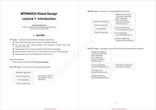
![3
2 MECHATRONICS
2.1 Difinition
Interdisciplinary field or engineering dealing with the design of products whose function relies on
the integration of mechanical and electronic components coordinated by a control architecture.
Originally introduced in Japan in early 1960’s, spread in Europe in late 1960’s and then in USA
in early 1970’s.
Primary disciplines – Mechanics, electronics, controls and computer engineering
Examples of Mechatronics systems
Aercraft flight control and navigation system
Automobile electronic fuel injection and antilock brake systems
Numerically controlled (NC) machine tools
Robots
Smart kitchen
Toys, etc
Figure 1.1 illustrates all the components in a typical mechatronic system.
Actuators – produce motion or cause some action
Sensors – detect the state of the system parameters, inputs and outputs
Digital devices – control the system
Conditioning and interfacing circuits – provide connections between the control
circuits and the input/output devices
Graphical displays – provide visual feedback to users
4
3 ROBOTS
3.1 Difinition
A reprogrammable, multifunctional manipulator designed to move material, parts, tools, or
specialized devices through various programmed motions for the performance of a variety of tasks.
A more inspiring definition can be found in Webster. According to Webster a robot is:
An automatic device that performs functions normally ascribed to humans or a machine in the
form of a human.
3.2 History
First use of the word 'robot'
The acclaimed Czech playwright Karel Capek (1890-1938) made the first use of the word ‘robot’,
from the Czech word for forced labor or serf. Capek was reportedly several times a candidate for the
Nobel prize for his works and very influential and prolific as a writer and playwright.
The use of the word Robot was introduced into his play R.U.R. (Rossum's Universal Robots) which
opened in Prague in January 1921.
In R.U.R., Capek poses a paradise, where the machines initially bring so many benefits but in the
end bring an equal amount of blight in the form of unemployment and social unrest.
The play was an enormous success and productions soon opened throughout Europe and the U.S.
R.U.R's theme, in part, was the dehumanization of man in a technological civilization.
You may find it surprising that the robots were not mechanical in nature but were created through chemical means. In
fact, in an essay written in 1935, Capek strongly fought that this idea was at all possible and, writing in the third person,
said:
"It is with horror, frankly, that he rejects all responsibility for the idea that metal contraptions could ever replace human
beings, and that by means of wires they could awaken something like life, love, or rebellion. He would deem this dark
prospect to be either an overestimation of machines, or a grave offence against life."
[The Author of Robots Defends Himself - Karl Capek, Lidove noviny, June 9, 1935, translation: Bean Comrada]
There is some evidence that the word robot was actually coined by Karl's brother Josef, a writer in his own right. In a
short letter, Capek writes that he asked Josef what he should call the artificial workers in his new play.
Karel suggests Labori, which he thinks too 'bookish' and his brother mutters "then call them Robots" and turns back to
his work, and so from a curt response we have the word robot.
CuuDuongThanCong.com https://fb.com/tailieudientucntt
c
u
u
d
u
o
n
g
t
h
a
n
c
o
n
g
.
c
o
m](data:image/gif;base64,R0lGODlhAQABAIAAAAAAAP///yH5BAEAAAAALAAAAAABAAEAAAIBRAA7)