SlideShare a Scribd company logo
1 of 11
Upper and Lower Bounds for Roots 3.5: More on Zeros of Polynomial Functions The Upper  and  Lower  Bound  Theorem  helps us rule out many of a polynomial equation's possible rational roots. The Upper  and  Lower  Bound  Theorem   Let   f   ( x )   be a polynomial with real coefficients and a positive leading coefficient, and let  a  and  b  be nonzero real numbers.  1.   Divide  f   ( x ) by  x    b  (where  b     0) using synthetic division. If the last row  containing the quotient and remainder has no negative numbers, then  b  is  an  upper  bound  for the real roots of  f   ( x )      0. 2.   Divide   f   ( x )   by  x    a  (where  a     0) using synthetic division. If the last row  containing the quotient and remainder has numbers that alternate in sign  (zero entries count as positive or negative), then  a  is a  lower  bound  for  the real roots of  f   ( x )      0.
EXAMPLE:   Finding Bounds for the Roots Show that all the real roots of the equation 8 x 3      10 x 2    39 x  + 9    0 lie between –3 and 2. Solution   We begin by showing that 2 is an upper bound. Divide the polynomial by  x      2. If all the numbers in the bottom row of the synthetic division are non­negative, then 2 is an upper bound .  All numbers in this row are nonnegative. 3.5: More on Zeros of Polynomial Functions 35 13 26 8 26 52 16 9  39 10 8 2 more more
EXAMPLE:   Finding Bounds for the Roots Show that all the real roots of the equation 8 x 3      10 x 2    39 x  + 9    0 lie between –3 and 2. Solution   The nonnegative entries in the last row verify that 2 is an upper bound. Next, we show that   3 is a lower bound. Divide the polynomial by  x     (  3), or  x     3. If the numbers in the bottom row of the synthetic division alternate in sign, then   3 is a lower bound. Remember that the number zero can be considered positive or negative.  Counting zero as negative, the signs alternate:   ,   ,   ,   . By the Upper and Lower Bound Theorem, the alternating signs in the last row indicate that   3 is a lower bound for the roots. (The zero remainder indicates that   3 is also a root.)  3.5: More on Zeros of Polynomial Functions 35 13 26 8  9 42  24 9  39 10 8  3
The Intermediate Value Theorem   The Intermediate Value Theorem for Polynomials Let  f   ( x ) be a polynomial function with real coefficients. If  f   ( a ) and  f   ( b )   have opposite signs, then there is at least one value of  c  between  a  and  b  for which  f   ( c ) = 0. Equivalently, the equation  f   ( x )    0 has at least one real root between  a  and  b .  3.5: More on Zeros of Polynomial Functions
EXAMPLE : Approximating a Real Zero a.   Show that the polynomial function  f   ( x )     x 3      2 x     5   has a real zero      between 2 and 3.  b.   Use the Intermediate Value Theorem to find an approximation for this    real zero to the nearest tenth  3.5: More on Zeros of Polynomial Functions a.   Let us evaluate  f   ( x )   at 2 and 3. If  f   (2) and  f   (3) have opposite signs, then  there is a real zero between 2 and 3. Using  f   ( x )      x 3      2 x     5, we obtain Solution This sign change shows that the polynomial function has a real zero  between 2 and 3.  and f   (3)     3 3      2    3    5    27    6    5   16. f   (3) is positive.   f   (2)     2 3      2    2    5    8    4    5   1 f  (2) is negative.
EXAMPLE : Approximating a Real Zero b.   A numerical approach is to evaluate  f   at successive tenths between 2 and  3, looking for a sign change. This sign change will place the real zero  between a pair of successive tenths.  Solution a.   Show that the polynomial function  f   ( x )     x 3      2 x     5   has a real zero      between 2 and 3.  b.   Use the Intermediate Value Theorem to find an approximation for this    real zero to the nearest tenth  The sign change indicates that  f  has a real zero between 2 and 2.1.  Sign change Sign change 3.5: More on Zeros of Polynomial Functions f   (2.1)     (2.1) 3      2(2.1)    5     0.061 2.1 f   (2)     2 3      2(2)    5       1 2 f   ( x )     x 3      2 x     5 x more more
EXAMPLE : Approximating a Real Zero b.   We now follow a similar procedure to locate the real zero between  successive hundredths. We divide the interval [2, 2.1] into ten equal sub- intervals. Then we evaluate  f  at each endpoint and look for a sign change. Solution a.   Show that the polynomial function  f   ( x )     x 3      2 x     5   has a real zero      between 2 and 3.  b.   Use the Intermediate Value Theorem to find an approximation for this    real zero to the nearest tenth  The sign change indicates that  f   has a real zero between 2.09 and 2.1.  Correct to the nearest tenth, the zero is 2.1.  Sign change 3.5: More on Zeros of Polynomial Functions f  (2.07)   0.270257 f  (2.03)   0.694573 f   (2.1)    0.061 f   (2.06)   0.378184 f   (2.02)   0.797592 f   (2.09)   0.050671 f  (2.05)   0.484875 f  (2.01)   0.899399 f  (2.08)   0.161088 f  (2.04)   0.590336 f   (2.00)   1
The Fundamental Theorem of Algebra 3.5: More on Zeros of Polynomial Functions We have seen that if a polynomial equation is of degree  n,  then counting multiple roots separately, the equation has  n  roots. This result is called the  Fundamental Theorem of Algebra. The Fundamental Theorem of Algebra  If  f   ( x ) is a polynomial of degree  n,  where  n     1, then the equation  f   ( x )    0 has at least one complex root.
The Linear Factorization Theorem   The Linear Factorization Theorem  If  f   ( x )      a n x n     a n  1 x n  1     …     a 1 x    a 0  b, where n    1 and  a n     0 , then f  ( x )      a n   ( x    c 1 ) ( x    c 2 )  …  ( x    c n )  where  c 1 ,  c 2 ,…,  c n  are complex numbers (possibly real and not necessarily distinct). In words: An  n th-degree polynomial can be expressed as the product of  n  linear factors.  Just as an  n th-degree polynomial equation has  n  roots, an  n th-degree polynomial has  n  linear factors. This is formally stated as the  Linear Factorization Theorem. 3.5: More on Zeros of Polynomial Functions
3.5: More on Zeros of Polynomial Functions EXAMPLE: Finding  a Polynomial  Function with Given Zeros   Find a fourth-degree polynomial function  f   ( x ) with real coefficients that has  2, and  i  as zeros and such that  f   (3)   150. Solution   Because  i   is a zero and the polynomial has real coefficients, the conjugate must also be a zero. We can now use the Linear Factorization Theorem.     a n ( x     2)( x    2)( x      i )( x      i ) Use the given zeros:  c 1    2,  c 2     2,  c 3      i , and, from above,  c 4    i .  f   ( x )      a n ( x    c 1 )( x    c 2 )( x    c 3 )( x    c 4 ) This is the linear factorization for a fourth-degree polynomial.      a n ( x 2     4)( x 2      i )    Multiply f   ( x )    a n ( x 4     3 x 2     4)    Complete the multiplication more more
3.5: More on Zeros of Polynomial Functions EXAMPLE: Finding  a Polynomial  Function with Given Zeros   Find a fourth-degree polynomial function  f   ( x ) with real coefficients that has  2, and  i  as zeros and such that  f   (3)   150. Substituting   3   for  a n   in the formula for  f   ( x ) ,  we obtain f   ( x )   3( x 4     3 x 2     4) .   Equivalently,  f   ( x )   3 x 4     9 x 2     12. Solution f  (3)     a n (3 4     3    3 2     4)   150     To find  a n , use the fact that  f  (3)   150. a n (81    27    4)   150   Solve for  a n .  50 a n    150 a n    3

More Related Content

What's hot

Regulafalsi_bydinesh
Regulafalsi_bydineshRegulafalsi_bydinesh
Regulafalsi_bydineshDinesh Kumar
 
Numerical Analysis (Solution of Non-Linear Equations) part 2
Numerical Analysis (Solution of Non-Linear Equations) part 2Numerical Analysis (Solution of Non-Linear Equations) part 2
Numerical Analysis (Solution of Non-Linear Equations) part 2Asad Ali
 
ROOT OF NON-LINEAR EQUATIONS
ROOT OF NON-LINEAR EQUATIONSROOT OF NON-LINEAR EQUATIONS
ROOT OF NON-LINEAR EQUATIONSfenil patel
 
3.4 Polynomial Functions and Their Graphs
3.4 Polynomial Functions and Their Graphs3.4 Polynomial Functions and Their Graphs
3.4 Polynomial Functions and Their Graphssmiller5
 
4.3 Logarithmic Functions
4.3 Logarithmic Functions4.3 Logarithmic Functions
4.3 Logarithmic Functionssmiller5
 
Mws gen nle_ppt_bisection
Mws gen nle_ppt_bisectionMws gen nle_ppt_bisection
Mws gen nle_ppt_bisectionAlvin Setiawan
 
Bracketing or closed methods
Bracketing or closed methodsBracketing or closed methods
Bracketing or closed methodsandrushow
 
Roots of equations
Roots of equationsRoots of equations
Roots of equationsRobinson
 
3.3 Zeros of Polynomial Functions
3.3 Zeros of Polynomial Functions3.3 Zeros of Polynomial Functions
3.3 Zeros of Polynomial Functionssmiller5
 
Roots of polynomials
Roots of polynomialsRoots of polynomials
Roots of polynomialsCesar Mendoza
 
2 1 polynomials
2 1 polynomials2 1 polynomials
2 1 polynomialshisema01
 

What's hot (20)

Regulafalsi_bydinesh
Regulafalsi_bydineshRegulafalsi_bydinesh
Regulafalsi_bydinesh
 
Numerical Analysis (Solution of Non-Linear Equations) part 2
Numerical Analysis (Solution of Non-Linear Equations) part 2Numerical Analysis (Solution of Non-Linear Equations) part 2
Numerical Analysis (Solution of Non-Linear Equations) part 2
 
Presentation aust final
Presentation aust finalPresentation aust final
Presentation aust final
 
ROOT OF NON-LINEAR EQUATIONS
ROOT OF NON-LINEAR EQUATIONSROOT OF NON-LINEAR EQUATIONS
ROOT OF NON-LINEAR EQUATIONS
 
3.4 Polynomial Functions and Their Graphs
3.4 Polynomial Functions and Their Graphs3.4 Polynomial Functions and Their Graphs
3.4 Polynomial Functions and Their Graphs
 
Bisection method
Bisection methodBisection method
Bisection method
 
4.3 Logarithmic Functions
4.3 Logarithmic Functions4.3 Logarithmic Functions
4.3 Logarithmic Functions
 
Mws gen nle_ppt_bisection
Mws gen nle_ppt_bisectionMws gen nle_ppt_bisection
Mws gen nle_ppt_bisection
 
Bracketing or closed methods
Bracketing or closed methodsBracketing or closed methods
Bracketing or closed methods
 
Roots of equations
Roots of equationsRoots of equations
Roots of equations
 
Unit 3.5
Unit 3.5Unit 3.5
Unit 3.5
 
Bisection
BisectionBisection
Bisection
 
3.3 Zeros of Polynomial Functions
3.3 Zeros of Polynomial Functions3.3 Zeros of Polynomial Functions
3.3 Zeros of Polynomial Functions
 
3.1
3.13.1
3.1
 
Roots of polynomials
Roots of polynomialsRoots of polynomials
Roots of polynomials
 
2 1 polynomials
2 1 polynomials2 1 polynomials
2 1 polynomials
 
Calc 4.4b
Calc 4.4bCalc 4.4b
Calc 4.4b
 
Roll's theorem
Roll's theoremRoll's theorem
Roll's theorem
 
newton raphson method
newton raphson methodnewton raphson method
newton raphson method
 
Mean value theorem
Mean value theoremMean value theorem
Mean value theorem
 

Viewers also liked

A26-7 Fundamental Thm of Algebra
A26-7 Fundamental Thm of AlgebraA26-7 Fundamental Thm of Algebra
A26-7 Fundamental Thm of Algebravhiggins1
 
Polynomial functions
Polynomial functionsPolynomial functions
Polynomial functionsMalikahmad105
 
A presentation on mathematicians
A presentation on mathematiciansA presentation on mathematicians
A presentation on mathematiciansShwetketu Rastogi
 
Famous mathematicians of all time
Famous mathematicians of all timeFamous mathematicians of all time
Famous mathematicians of all timeTejasav Khattar
 
Great mathematician
Great mathematicianGreat mathematician
Great mathematicianRajat Anand
 
5.6.08 Fundamental Theorem Of Algebra1
5.6.08   Fundamental Theorem Of Algebra15.6.08   Fundamental Theorem Of Algebra1
5.6.08 Fundamental Theorem Of Algebra1chrismac47
 

Viewers also liked (8)

2 5 zeros of poly fn
2 5 zeros of poly fn2 5 zeros of poly fn
2 5 zeros of poly fn
 
A26-7 Fundamental Thm of Algebra
A26-7 Fundamental Thm of AlgebraA26-7 Fundamental Thm of Algebra
A26-7 Fundamental Thm of Algebra
 
Unit 2.5
Unit 2.5Unit 2.5
Unit 2.5
 
Polynomial functions
Polynomial functionsPolynomial functions
Polynomial functions
 
A presentation on mathematicians
A presentation on mathematiciansA presentation on mathematicians
A presentation on mathematicians
 
Famous mathematicians of all time
Famous mathematicians of all timeFamous mathematicians of all time
Famous mathematicians of all time
 
Great mathematician
Great mathematicianGreat mathematician
Great mathematician
 
5.6.08 Fundamental Theorem Of Algebra1
5.6.08   Fundamental Theorem Of Algebra15.6.08   Fundamental Theorem Of Algebra1
5.6.08 Fundamental Theorem Of Algebra1
 

Similar to The fundamental thorem of algebra

Polynomial functions modelllings
Polynomial functions modelllingsPolynomial functions modelllings
Polynomial functions modelllingsTarun Gehlot
 
3.4 Polynomial Functions and Their Graphs
3.4 Polynomial Functions and Their Graphs3.4 Polynomial Functions and Their Graphs
3.4 Polynomial Functions and Their Graphssmiller5
 
APPLICATION OF PARTIAL DIFFERENTIATION
APPLICATION OF PARTIAL DIFFERENTIATIONAPPLICATION OF PARTIAL DIFFERENTIATION
APPLICATION OF PARTIAL DIFFERENTIATIONDhrupal Patel
 
Mac2311 study guide-tcm6-49721
Mac2311 study guide-tcm6-49721Mac2311 study guide-tcm6-49721
Mac2311 study guide-tcm6-49721Glicerio Gavilan
 
Synthetic and Remainder Theorem of Polynomials.ppt
Synthetic and Remainder Theorem of Polynomials.pptSynthetic and Remainder Theorem of Polynomials.ppt
Synthetic and Remainder Theorem of Polynomials.pptMarkVincentDoria1
 
Module 3 polynomial functions
Module 3   polynomial functionsModule 3   polynomial functions
Module 3 polynomial functionsdionesioable
 
Solution of nonlinear_equations
Solution of nonlinear_equationsSolution of nonlinear_equations
Solution of nonlinear_equationsTarun Gehlot
 
5.5 Zeros of Polynomial Functions
5.5 Zeros of Polynomial Functions5.5 Zeros of Polynomial Functions
5.5 Zeros of Polynomial Functionssmiller5
 
Create a polynomial function that meets the following conditions- Expl.docx
Create a polynomial function that meets the following conditions- Expl.docxCreate a polynomial function that meets the following conditions- Expl.docx
Create a polynomial function that meets the following conditions- Expl.docxmrichard5
 
Making Connections
Making ConnectionsMaking Connections
Making ConnectionsKristen T
 
Numarical values
Numarical valuesNumarical values
Numarical valuesAmanSaeed11
 
Numarical values highlighted
Numarical values highlightedNumarical values highlighted
Numarical values highlightedAmanSaeed11
 
3 2 Polynomial Functions And Their Graphs
3 2 Polynomial Functions And Their Graphs3 2 Polynomial Functions And Their Graphs
3 2 Polynomial Functions And Their Graphssilvia
 

Similar to The fundamental thorem of algebra (20)

Polynomial functions modelllings
Polynomial functions modelllingsPolynomial functions modelllings
Polynomial functions modelllings
 
3.4 Polynomial Functions and Their Graphs
3.4 Polynomial Functions and Their Graphs3.4 Polynomial Functions and Their Graphs
3.4 Polynomial Functions and Their Graphs
 
APPLICATION OF PARTIAL DIFFERENTIATION
APPLICATION OF PARTIAL DIFFERENTIATIONAPPLICATION OF PARTIAL DIFFERENTIATION
APPLICATION OF PARTIAL DIFFERENTIATION
 
Ch 2
Ch 2Ch 2
Ch 2
 
Mac2311 study guide-tcm6-49721
Mac2311 study guide-tcm6-49721Mac2311 study guide-tcm6-49721
Mac2311 study guide-tcm6-49721
 
Synthetic and Remainder Theorem of Polynomials.ppt
Synthetic and Remainder Theorem of Polynomials.pptSynthetic and Remainder Theorem of Polynomials.ppt
Synthetic and Remainder Theorem of Polynomials.ppt
 
Module 3 polynomial functions
Module 3   polynomial functionsModule 3   polynomial functions
Module 3 polynomial functions
 
Solution of nonlinear_equations
Solution of nonlinear_equationsSolution of nonlinear_equations
Solution of nonlinear_equations
 
5.5 Zeros of Polynomial Functions
5.5 Zeros of Polynomial Functions5.5 Zeros of Polynomial Functions
5.5 Zeros of Polynomial Functions
 
3
33
3
 
Create a polynomial function that meets the following conditions- Expl.docx
Create a polynomial function that meets the following conditions- Expl.docxCreate a polynomial function that meets the following conditions- Expl.docx
Create a polynomial function that meets the following conditions- Expl.docx
 
Unit 2.4
Unit 2.4Unit 2.4
Unit 2.4
 
Unit 2.3
Unit 2.3Unit 2.3
Unit 2.3
 
Lemh105
Lemh105Lemh105
Lemh105
 
Making Connections
Making ConnectionsMaking Connections
Making Connections
 
OPERATIONS RESEARCH
OPERATIONS RESEARCHOPERATIONS RESEARCH
OPERATIONS RESEARCH
 
Numarical values
Numarical valuesNumarical values
Numarical values
 
Numarical values highlighted
Numarical values highlightedNumarical values highlighted
Numarical values highlighted
 
Unit-8.pdf
Unit-8.pdfUnit-8.pdf
Unit-8.pdf
 
3 2 Polynomial Functions And Their Graphs
3 2 Polynomial Functions And Their Graphs3 2 Polynomial Functions And Their Graphs
3 2 Polynomial Functions And Their Graphs
 

Recently uploaded

Paris 2024 Olympic Geographies - an activity
Paris 2024 Olympic Geographies - an activityParis 2024 Olympic Geographies - an activity
Paris 2024 Olympic Geographies - an activityGeoBlogs
 
Sports & Fitness Value Added Course FY..
Sports & Fitness Value Added Course FY..Sports & Fitness Value Added Course FY..
Sports & Fitness Value Added Course FY..Disha Kariya
 
BASLIQ CURRENT LOOKBOOK LOOKBOOK(1) (1).pdf
BASLIQ CURRENT LOOKBOOK  LOOKBOOK(1) (1).pdfBASLIQ CURRENT LOOKBOOK  LOOKBOOK(1) (1).pdf
BASLIQ CURRENT LOOKBOOK LOOKBOOK(1) (1).pdfSoniaTolstoy
 
Kisan Call Centre - To harness potential of ICT in Agriculture by answer farm...
Kisan Call Centre - To harness potential of ICT in Agriculture by answer farm...Kisan Call Centre - To harness potential of ICT in Agriculture by answer farm...
Kisan Call Centre - To harness potential of ICT in Agriculture by answer farm...Krashi Coaching
 
Accessible design: Minimum effort, maximum impact
Accessible design: Minimum effort, maximum impactAccessible design: Minimum effort, maximum impact
Accessible design: Minimum effort, maximum impactdawncurless
 
Beyond the EU: DORA and NIS 2 Directive's Global Impact
Beyond the EU: DORA and NIS 2 Directive's Global ImpactBeyond the EU: DORA and NIS 2 Directive's Global Impact
Beyond the EU: DORA and NIS 2 Directive's Global ImpactPECB
 
BAG TECHNIQUE Bag technique-a tool making use of public health bag through wh...
BAG TECHNIQUE Bag technique-a tool making use of public health bag through wh...BAG TECHNIQUE Bag technique-a tool making use of public health bag through wh...
BAG TECHNIQUE Bag technique-a tool making use of public health bag through wh...Sapna Thakur
 
microwave assisted reaction. General introduction
microwave assisted reaction. General introductionmicrowave assisted reaction. General introduction
microwave assisted reaction. General introductionMaksud Ahmed
 
General AI for Medical Educators April 2024
General AI for Medical Educators April 2024General AI for Medical Educators April 2024
General AI for Medical Educators April 2024Janet Corral
 
The Most Excellent Way | 1 Corinthians 13
The Most Excellent Way | 1 Corinthians 13The Most Excellent Way | 1 Corinthians 13
The Most Excellent Way | 1 Corinthians 13Steve Thomason
 
Presentation by Andreas Schleicher Tackling the School Absenteeism Crisis 30 ...
Presentation by Andreas Schleicher Tackling the School Absenteeism Crisis 30 ...Presentation by Andreas Schleicher Tackling the School Absenteeism Crisis 30 ...
Presentation by Andreas Schleicher Tackling the School Absenteeism Crisis 30 ...EduSkills OECD
 
Introduction to Nonprofit Accounting: The Basics
Introduction to Nonprofit Accounting: The BasicsIntroduction to Nonprofit Accounting: The Basics
Introduction to Nonprofit Accounting: The BasicsTechSoup
 
SOCIAL AND HISTORICAL CONTEXT - LFTVD.pptx
SOCIAL AND HISTORICAL CONTEXT - LFTVD.pptxSOCIAL AND HISTORICAL CONTEXT - LFTVD.pptx
SOCIAL AND HISTORICAL CONTEXT - LFTVD.pptxiammrhaywood
 
Explore beautiful and ugly buildings. Mathematics helps us create beautiful d...
Explore beautiful and ugly buildings. Mathematics helps us create beautiful d...Explore beautiful and ugly buildings. Mathematics helps us create beautiful d...
Explore beautiful and ugly buildings. Mathematics helps us create beautiful d...christianmathematics
 
Interactive Powerpoint_How to Master effective communication
Interactive Powerpoint_How to Master effective communicationInteractive Powerpoint_How to Master effective communication
Interactive Powerpoint_How to Master effective communicationnomboosow
 
Z Score,T Score, Percential Rank and Box Plot Graph
Z Score,T Score, Percential Rank and Box Plot GraphZ Score,T Score, Percential Rank and Box Plot Graph
Z Score,T Score, Percential Rank and Box Plot GraphThiyagu K
 
APM Welcome, APM North West Network Conference, Synergies Across Sectors
APM Welcome, APM North West Network Conference, Synergies Across SectorsAPM Welcome, APM North West Network Conference, Synergies Across Sectors
APM Welcome, APM North West Network Conference, Synergies Across SectorsAssociation for Project Management
 
Nutritional Needs Presentation - HLTH 104
Nutritional Needs Presentation - HLTH 104Nutritional Needs Presentation - HLTH 104
Nutritional Needs Presentation - HLTH 104misteraugie
 

Recently uploaded (20)

Paris 2024 Olympic Geographies - an activity
Paris 2024 Olympic Geographies - an activityParis 2024 Olympic Geographies - an activity
Paris 2024 Olympic Geographies - an activity
 
Sports & Fitness Value Added Course FY..
Sports & Fitness Value Added Course FY..Sports & Fitness Value Added Course FY..
Sports & Fitness Value Added Course FY..
 
BASLIQ CURRENT LOOKBOOK LOOKBOOK(1) (1).pdf
BASLIQ CURRENT LOOKBOOK  LOOKBOOK(1) (1).pdfBASLIQ CURRENT LOOKBOOK  LOOKBOOK(1) (1).pdf
BASLIQ CURRENT LOOKBOOK LOOKBOOK(1) (1).pdf
 
Kisan Call Centre - To harness potential of ICT in Agriculture by answer farm...
Kisan Call Centre - To harness potential of ICT in Agriculture by answer farm...Kisan Call Centre - To harness potential of ICT in Agriculture by answer farm...
Kisan Call Centre - To harness potential of ICT in Agriculture by answer farm...
 
Accessible design: Minimum effort, maximum impact
Accessible design: Minimum effort, maximum impactAccessible design: Minimum effort, maximum impact
Accessible design: Minimum effort, maximum impact
 
Beyond the EU: DORA and NIS 2 Directive's Global Impact
Beyond the EU: DORA and NIS 2 Directive's Global ImpactBeyond the EU: DORA and NIS 2 Directive's Global Impact
Beyond the EU: DORA and NIS 2 Directive's Global Impact
 
BAG TECHNIQUE Bag technique-a tool making use of public health bag through wh...
BAG TECHNIQUE Bag technique-a tool making use of public health bag through wh...BAG TECHNIQUE Bag technique-a tool making use of public health bag through wh...
BAG TECHNIQUE Bag technique-a tool making use of public health bag through wh...
 
microwave assisted reaction. General introduction
microwave assisted reaction. General introductionmicrowave assisted reaction. General introduction
microwave assisted reaction. General introduction
 
General AI for Medical Educators April 2024
General AI for Medical Educators April 2024General AI for Medical Educators April 2024
General AI for Medical Educators April 2024
 
The Most Excellent Way | 1 Corinthians 13
The Most Excellent Way | 1 Corinthians 13The Most Excellent Way | 1 Corinthians 13
The Most Excellent Way | 1 Corinthians 13
 
Presentation by Andreas Schleicher Tackling the School Absenteeism Crisis 30 ...
Presentation by Andreas Schleicher Tackling the School Absenteeism Crisis 30 ...Presentation by Andreas Schleicher Tackling the School Absenteeism Crisis 30 ...
Presentation by Andreas Schleicher Tackling the School Absenteeism Crisis 30 ...
 
Introduction to Nonprofit Accounting: The Basics
Introduction to Nonprofit Accounting: The BasicsIntroduction to Nonprofit Accounting: The Basics
Introduction to Nonprofit Accounting: The Basics
 
SOCIAL AND HISTORICAL CONTEXT - LFTVD.pptx
SOCIAL AND HISTORICAL CONTEXT - LFTVD.pptxSOCIAL AND HISTORICAL CONTEXT - LFTVD.pptx
SOCIAL AND HISTORICAL CONTEXT - LFTVD.pptx
 
Explore beautiful and ugly buildings. Mathematics helps us create beautiful d...
Explore beautiful and ugly buildings. Mathematics helps us create beautiful d...Explore beautiful and ugly buildings. Mathematics helps us create beautiful d...
Explore beautiful and ugly buildings. Mathematics helps us create beautiful d...
 
Interactive Powerpoint_How to Master effective communication
Interactive Powerpoint_How to Master effective communicationInteractive Powerpoint_How to Master effective communication
Interactive Powerpoint_How to Master effective communication
 
Z Score,T Score, Percential Rank and Box Plot Graph
Z Score,T Score, Percential Rank and Box Plot GraphZ Score,T Score, Percential Rank and Box Plot Graph
Z Score,T Score, Percential Rank and Box Plot Graph
 
Mattingly "AI & Prompt Design: Structured Data, Assistants, & RAG"
Mattingly "AI & Prompt Design: Structured Data, Assistants, & RAG"Mattingly "AI & Prompt Design: Structured Data, Assistants, & RAG"
Mattingly "AI & Prompt Design: Structured Data, Assistants, & RAG"
 
APM Welcome, APM North West Network Conference, Synergies Across Sectors
APM Welcome, APM North West Network Conference, Synergies Across SectorsAPM Welcome, APM North West Network Conference, Synergies Across Sectors
APM Welcome, APM North West Network Conference, Synergies Across Sectors
 
Mattingly "AI & Prompt Design: The Basics of Prompt Design"
Mattingly "AI & Prompt Design: The Basics of Prompt Design"Mattingly "AI & Prompt Design: The Basics of Prompt Design"
Mattingly "AI & Prompt Design: The Basics of Prompt Design"
 
Nutritional Needs Presentation - HLTH 104
Nutritional Needs Presentation - HLTH 104Nutritional Needs Presentation - HLTH 104
Nutritional Needs Presentation - HLTH 104
 

The fundamental thorem of algebra

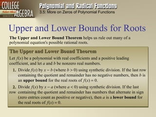
  • 1. Upper and Lower Bounds for Roots 3.5: More on Zeros of Polynomial Functions The Upper and Lower Bound Theorem helps us rule out many of a polynomial equation's possible rational roots. The Upper and Lower Bound Theorem Let f ( x ) be a polynomial with real coefficients and a positive leading coefficient, and let a and b be nonzero real numbers. 1. Divide f ( x ) by x  b (where b  0) using synthetic division. If the last row containing the quotient and remainder has no negative numbers, then b is an upper bound for the real roots of f ( x )  0. 2. Divide f ( x ) by x  a (where a  0) using synthetic division. If the last row containing the quotient and remainder has numbers that alternate in sign (zero entries count as positive or negative), then a is a lower bound for the real roots of f ( x )  0.
  • 2. EXAMPLE: Finding Bounds for the Roots Show that all the real roots of the equation 8 x 3  10 x 2  39 x + 9  0 lie between –3 and 2. Solution We begin by showing that 2 is an upper bound. Divide the polynomial by x  2. If all the numbers in the bottom row of the synthetic division are non­negative, then 2 is an upper bound . All numbers in this row are nonnegative. 3.5: More on Zeros of Polynomial Functions 35 13 26 8 26 52 16 9  39 10 8 2 more more
  • 3. EXAMPLE: Finding Bounds for the Roots Show that all the real roots of the equation 8 x 3  10 x 2  39 x + 9  0 lie between –3 and 2. Solution The nonnegative entries in the last row verify that 2 is an upper bound. Next, we show that  3 is a lower bound. Divide the polynomial by x  (  3), or x  3. If the numbers in the bottom row of the synthetic division alternate in sign, then  3 is a lower bound. Remember that the number zero can be considered positive or negative. Counting zero as negative, the signs alternate:  ,  ,  ,  . By the Upper and Lower Bound Theorem, the alternating signs in the last row indicate that  3 is a lower bound for the roots. (The zero remainder indicates that  3 is also a root.) 3.5: More on Zeros of Polynomial Functions 35 13 26 8  9 42  24 9  39 10 8  3
  • 4. The Intermediate Value Theorem The Intermediate Value Theorem for Polynomials Let f ( x ) be a polynomial function with real coefficients. If f ( a ) and f ( b ) have opposite signs, then there is at least one value of c between a and b for which f ( c ) = 0. Equivalently, the equation f ( x )  0 has at least one real root between a and b . 3.5: More on Zeros of Polynomial Functions
  • 5. EXAMPLE : Approximating a Real Zero a. Show that the polynomial function f ( x )  x 3  2 x  5 has a real zero between 2 and 3. b. Use the Intermediate Value Theorem to find an approximation for this real zero to the nearest tenth 3.5: More on Zeros of Polynomial Functions a. Let us evaluate f ( x ) at 2 and 3. If f (2) and f (3) have opposite signs, then there is a real zero between 2 and 3. Using f ( x )  x 3  2 x  5, we obtain Solution This sign change shows that the polynomial function has a real zero between 2 and 3. and f (3)  3 3  2  3  5  27  6  5  16. f (3) is positive. f (2)  2 3  2  2  5  8  4  5  1 f (2) is negative.
  • 6. EXAMPLE : Approximating a Real Zero b. A numerical approach is to evaluate f at successive tenths between 2 and 3, looking for a sign change. This sign change will place the real zero between a pair of successive tenths. Solution a. Show that the polynomial function f ( x )  x 3  2 x  5 has a real zero between 2 and 3. b. Use the Intermediate Value Theorem to find an approximation for this real zero to the nearest tenth The sign change indicates that f has a real zero between 2 and 2.1. Sign change Sign change 3.5: More on Zeros of Polynomial Functions f (2.1)  (2.1) 3  2(2.1)  5  0.061 2.1 f (2)  2 3  2(2)  5   1 2 f ( x )  x 3  2 x  5 x more more
  • 7. EXAMPLE : Approximating a Real Zero b. We now follow a similar procedure to locate the real zero between successive hundredths. We divide the interval [2, 2.1] into ten equal sub- intervals. Then we evaluate f at each endpoint and look for a sign change. Solution a. Show that the polynomial function f ( x )  x 3  2 x  5 has a real zero between 2 and 3. b. Use the Intermediate Value Theorem to find an approximation for this real zero to the nearest tenth The sign change indicates that f has a real zero between 2.09 and 2.1. Correct to the nearest tenth, the zero is 2.1. Sign change 3.5: More on Zeros of Polynomial Functions f (2.07)  0.270257 f (2.03)  0.694573 f (2.1)  0.061 f (2.06)  0.378184 f (2.02)  0.797592 f (2.09)  0.050671 f (2.05)  0.484875 f (2.01)  0.899399 f (2.08)  0.161088 f (2.04)  0.590336 f (2.00)  1
  • 8. The Fundamental Theorem of Algebra 3.5: More on Zeros of Polynomial Functions We have seen that if a polynomial equation is of degree n, then counting multiple roots separately, the equation has n roots. This result is called the Fundamental Theorem of Algebra. The Fundamental Theorem of Algebra If f ( x ) is a polynomial of degree n, where n  1, then the equation f ( x )  0 has at least one complex root.
  • 9. The Linear Factorization Theorem The Linear Factorization Theorem If f ( x )  a n x n  a n  1 x n  1   …  a 1 x  a 0 b, where n  1 and a n  0 , then f ( x )  a n ( x  c 1 ) ( x  c 2 ) … ( x  c n ) where c 1 , c 2 ,…, c n are complex numbers (possibly real and not necessarily distinct). In words: An n th-degree polynomial can be expressed as the product of n linear factors. Just as an n th-degree polynomial equation has n roots, an n th-degree polynomial has n linear factors. This is formally stated as the Linear Factorization Theorem. 3.5: More on Zeros of Polynomial Functions
  • 10. 3.5: More on Zeros of Polynomial Functions EXAMPLE: Finding a Polynomial Function with Given Zeros Find a fourth-degree polynomial function f ( x ) with real coefficients that has  2, and i as zeros and such that f (3)  150. Solution Because i is a zero and the polynomial has real coefficients, the conjugate must also be a zero. We can now use the Linear Factorization Theorem.  a n ( x  2)( x  2)( x  i )( x  i ) Use the given zeros: c 1  2, c 2  2, c 3  i , and, from above, c 4  i . f ( x )  a n ( x  c 1 )( x  c 2 )( x  c 3 )( x  c 4 ) This is the linear factorization for a fourth-degree polynomial.  a n ( x 2  4)( x 2  i ) Multiply f ( x )  a n ( x 4  3 x 2  4) Complete the multiplication more more
  • 11. 3.5: More on Zeros of Polynomial Functions EXAMPLE: Finding a Polynomial Function with Given Zeros Find a fourth-degree polynomial function f ( x ) with real coefficients that has  2, and i as zeros and such that f (3)  150. Substituting  3 for a n in the formula for f ( x ) , we obtain f ( x )  3( x 4  3 x 2  4) . Equivalently, f ( x )  3 x 4  9 x 2  12. Solution f (3)  a n (3 4  3  3 2  4)  150 To find a n , use the fact that f (3)  150. a n (81  27  4)  150 Solve for a n . 50 a n  150 a n  3