1. Chapter 5
Applications of the definite integral to
calculating volume and length
In this chapter we consider applications of the definite integral to calculating geometric quantities
such as volumes. The idea will be to dissect the three dimensional objects into pieces that resemble
disks or shells, whose volumes we can approximate with simple formulae. The volume of the entire
object is obtained by summing up volumes of a stack of disks or a set of embedded shells, and
considering the limit as the thickness of the dissection cuts gets thinner.
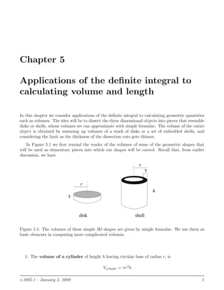
In Figure 5.1 we first remind the reader of the volumes of some of the geometric shapes that
will be used as elementary pieces into which our shapes will be carved. Recall that, from earlier
discussion, we have
r
h
τ
r
τ
disk shell
Figure 5.1: The volumes of these simple 3D shapes are given by simple formulae. We use them as
basic elements in computing more complicated volumes.
1. The volume of a cylinder of height h having circular base of radius r, is
Vcylinder = πr2
h
v.2005.1 - January 5, 2009 1
2. Math 103 Notes Chapter 5
2. The volume of a circular disk of thickness τ, and radius r (shown in Figure 5.1 a), as a special
case of the above, is
Vdisk = πr2
τ.
3. The volume of a cylindrical shell of height h, with circular radius r and small thickness τ
(shown in Figure 5.1 b) is
Vshell = 2πrhτ.
(This approximation holds for τ << r.)
5.1 Solids of revolution
In our first approach to volumes, we will restrict attention to solids of revolution, i.e. volumes
enclosed by some curve (described by a function such as y = f(x)), when it is rotated about one of
the axes. In Figure 5.2(a) we show one such curve, and the surface it forms when it is revolved about
the x axis. We note that if this surface is cut into slices along the x axis, the cross-sections look like
circles. (The circle will have a radius that depends on the position of the cut.) In Figure 5.2(b) we
show how a set of disks of various radii can approximately represent the shape of interest. The total
(a)
(b)
r
∆ x
y=f(x)
Figure 5.2: (a) A solid of revolution, showing dissection into slices along its axis of rotation. (b)
The same volume is approximated by a set of disks. Each disk has some radius r (that varies along
the length of the object) and thickness ∆x. Note that the thickness is in the direction of the x axis:
this will remind us that we integrate with respect to x.
volume of these disks is not the same, clearly, as the volume of the object, since some of these stick
out beyond the surface. However, if we make the thickness of these disks very small, we will get a
v.2005.1 - January 5, 2009 2
3. Math 103 Notes Chapter 5
good approximation of the desired volume. In the limit, as the thickness becomes infinitesimal, we
arrive at the true volume.
In most of the examples discussed in this chapter, the key step is to make careful observation
of the way that the radius of a given disk depends on the function that generates the surface. (By
this we mean the function that specifies the curve that forms the surface of revolution.) We also
pay attention to the dimension that forms the disk thickness.
Some of our examples will involve surfaces revolved about the x axis, and others will be revolved
about the y axis. In setting up these examples, a diagram is usually quite helpful.
Example 1: Volume of a sphere
∆ x
y
x
∆ x
x
f(x )
k
k
Figure 5.3: When the semicircle (on the left) is rotated about the x axis, it generates a sphere. On
the right, we show one disk generated by the revolution of the shaded rectangle.
We can think of a sphere of radius R as a solid formed by rotating a semi-circle about its long
axis. (See Figure 5.3.) A function that describe the semi-circle is
y = f(x) =
√
R2 − x2.
We show the sphere dissected into a set of disks, each of width ∆x. The disks are lined up along
the x axis with coordinates xk. These are just integer multiples of the slice thickness ∆x, so for
example,
xk = k∆x .
The radius of the disk depends on its position. Indeed, the radius of a disk through the x axis at a
point xk is specified by the function rk = yk = f(xk).
The volume of the k’th disk is
Vk = πr2
k∆x.
v.2005.1 - January 5, 2009 3
4. Math 103 Notes Chapter 5
By the above remarks, using the fact that the function actually determines the radius, we have
Vk = π(f(xk))2
∆x
Vk = π( R2 − x2
k)2
∆x = π(R2
− x2
k)∆x.
The total volume of all the disks is
V =
k
Vk = π(f(xk))2
∆x.
as ∆x → 0, this sum becomes a definite integral, and represents the true volume. We must ascertain
where to start and end the summation: i.e. the interval over which the disks are arranged. From
the figure, we note that the semi-circle extends from x = −R to x = R.
Thus
Vsphere =
R
-R
π(f(xk))2
dx = π
R
-R
(R2
− x2
) dx
We compute
Vsphere = π R2
x −
x3
3
R
-R
We can also make the observation that this is twice the volume obtained for the interval 0 < x < R,
Vsphere = 2π R2
x −
x3
3
R
0
= 2π R3
−
R3
3
After simplification, we arrive at the familiar formula
Vsphere =
4
3
πR3
Example 2: Volume of a paraboloid: disk method
Consider the curve
y = f(x) = 1 − x2
If we rotate this curve about the y axis, we will get a paraboloid as shown in Figure 5.4. In this
section we show how to compute the volume by dissecting into disks stacked up along the y axis.
Solution
The width of each disk is ∆y and, when taken to be very small, will become dy in the integral
below. The volume of each disk is
Vdisk = πr2
∆y
where the radius, r is now in the direction parallel to the x axis. Thus we express radius as
r = x = f(y).
v.2005.1 - January 5, 2009 4
5. Math 103 Notes Chapter 5
0
0.2
0.4
0.6
0.8
1
0.2 0.4 0.6 0.8 1
x
Figure 5.4: The curve that generates the shape of a paraboloid (left) and the shape of the paraboloid
(right).
We must express the equation of the curve in the form x as a function of y. From y = 1 − x2
we
have x2
= 1 − y so x =
√
1 − y. The shape extends from a smallest value of y = 0 up to y = 1.
Thus the volume is
V = π
1
0
[f(y)]2
dy = π
1
0
[ 1 − y]2
dy
We compute
V = π
1
0
(1 − y) dy = π y −
y2
2
1
0
V = π 1 −
1
2
=
π
2
.
The above example was set up using disks. However, there are other options. Below, we show
yet another method, comprised of cylindrical shells to compute the volume of a cone. In some cases,
one method is preferable to another, but here either method works equally well.
Example 3: Volume of cone: shell method
We use the shell method to find the volume of the cone formed by rotating the curve
y = 1 − x
about the y axis.
Solution
We show the cone and its generating curve in Figure 5.5, together with a representative shell used in
the calculation of total volume. The volume of a cylindrical shell of radius r, height h and thickness
τ is
Vshell = 2πrhτ.
v.2005.1 - January 5, 2009 5
6. Math 103 Notes Chapter 5
0
0.2
0.4
0.6
0.8
1
0.2 0.4 0.6 0.8 1
x
x
y
y=1−x
dx
Figure 5.5: Top: The curve that generates the cone (left) and the shape of the cone (right). Bottom:
the cone showing one of the series of shells that are used in this example to calculate its volume.
We will place these shells one inside the other so that their radii are parallel to the x axis (so r = x).
Then the heights of the shells are determined by the y value (i.e. h = y = 1 − x = 1 − r). For the
tallest shell r = 0, and for the flattest shell r = 1. The thickness of the shell is dr. Therefore, the
volume of one shell is
Vshell = 2πr(1 − r) dr.
The volume of the whole set of shells is obtained by integrating over 0 ≤ r ≤ 1, to obtain:
V = 2π
1
0
r(1 − r) dr = 2π
1
0
(r − r2
) dr.
We find that
V = 2π
r2
2
−
r3
3
1
0
= 2π
1
2
−
1
3
=
π
3
.
v.2005.1 - January 5, 2009 6
7. Math 103 Notes Chapter 5
Example 3
Find the volume of the surface formed by rotating the curve
y = f(x) =
√
x 0 < x < 1
(a) about the x axis. (b) about the y axis.
Solution
(a) If we rotate this curve about the x axis, we obtain a bowl shape; dissecting this surface leads
to disks stacked along the x axis, with thickness ∆x → dx, with radii in the y direction, i.e.
r = y = f(x), and with x in the range 0 < x < 1. The volume will thus be
V = π
1
0
[f(x)]2
dx = π
1
0
[
√
x]2
dx = π
1
0
x dx
Thus
V = π
x2
2
1
0
=
π
2
.
(b) When the curve is rotated about the y axis, it forms a surface with a sharp point at the
origin. The disks are stacked along the y axis, with thickness ∆y → dy, and radii in the x direction.
We must rewrite the function in the form
x = g(y) = y2
.
We now use the interval along the y axis, i.e. 0 < y < 1 The volume is then
V = π
1
0
[f(y)]2
dy = π
1
0
[y2
]2
dy = π
1
0
y4
dy.
V = π
y5
5
1
0
=
π
5
.
5.2 Mass and density
In the previous chapter, we introduced the idea of density in one dimension. Underlying the integral
we computed was the idea that the interval could be “dissected” into small parts (of width ∆x),
and a sum of pieces transformed into an integral. In the next examples, we consider similar ideas,
but instead of dissecting the region into 1-dimensional intervals, we have slightly more interesting
geometries.
v.2005.1 - January 5, 2009 7
8. Math 103 Notes Chapter 5
5.2.1 A glucose density gradient
A cylindrical test-tube of radius r, and height h, contains a solution of glucose which has been
prepared so that the concentration of glucose is greatest at the bottom and decreases gradually
towards the top of the tube. (This is called a density gradient). Suppose that the concentration c
as a function of the depth x is c(x) = 0.1 + 0.5x grams per centimeter3
. (x = 0 at the top of the
tube, and x = h at the bottom of the tube.) Determine the total amount of glucose in the tube (in
gm). neglect the “rounded” lower portion of the tube: i.e. assume that it is a simple cylinder.
In Figure 5.6 we show a rough version of what this gradient might look like. In reality, the
transition between high and low concentration would be smoother than shown in this figure.
x=0
r
x=h
∆ x
Figure 5.6: A test-tube of radius r containing a gradient of glucose. A disk-shaped slice of the tube
with small thickness ∆x has approximately constant density.
Solution
We assume a simple cylindrical tube and consider imaginary “slices” of this tube along its vertical
axis. Suppose that the thickness of a slice is ∆x. Then the volume of each of these (disk shaped)
slices is πr2
∆x. The amount of glucose in the slice is approximately equal to the concentration
c(x) multiplied by the volume of the slice, i.e. the small slice contains an amount πr2
∆xc(x) of
glucose. In order to sum up the total amount over all slices, we use a definite integral. (We imagine
∆x → dx becoming “infinitesimal” as the number of slices increases.) The integral we want is
G = πr2
h
0
c(x) dx.
Even though the geometry of the test-tube may, at first glance, seem more complicated than the
one-dimensional highway of the previous example, we observe here that the integral that computes
the total amount is still a sum over a single spatial variable, x. (Note the resemblance between the
integrals
I =
L
0
C(x) dx and G = πr2
h
0
c(x) dx
v.2005.1 - January 5, 2009 8
9. Math 103 Notes Chapter 5
here and in the previous problem.) We have neglected the complication of the rounded bottom
portion of the test-tube, so that integration over its length (which is actually summation of disks
shown in Figure 5.7) is a one-dimensional problem.
In this case the amount is
G = πr2
h
0
(0.1 + 0.5x)dx = πr2
0.1x +
0.5x2
2
h
0
= πr2
0.1h +
0.5h2
2
Suppose that the height of the test-tube is h = 10 cm and its radius is r = 1 cm. Then the total
mass of glucose in grams is
G = π 0.1(10) +
0.5(100)
2
= π (1 + 25) = 26π
In the next example, we consider a circular geometry, but the concept of dissecting and summing
is the same. Our task is to determine how to set up the problem in terms of an integral, and, again,
we must imagine which type of subdivision would lead to the summation (integration) needed to
compute total amount.
5.2.2 A circular colony of bacteria
Bacteria are growing in a circular colony with a radius of 1 cm. At distance r from the center of the
colony, the density of the bacteria, in units of one million cells per square centimeter, is observed
to be b(r) = 1 − r2
(Note: r is distance from the center in cm, so that 0 ≤ r ≤ 1). What is the
total number of bacteria in the colony?
∆ r
r
Side view
Top view (one ring)
Figure 5.7: A colony of bacteria with circular symmetry. A ring of small thickness ∆r has roughly
constant density.
Solution
Figure 5.7 shows a rough sketch of a petri dish with a colony of bacteria growing inside. The density
v.2005.1 - January 5, 2009 9
10. Math 103 Notes Chapter 5
0 r
b(r)
1
b(r)=1−r2
Figure 5.8: Bacterial density as a function of radius
as a function of distance from the center is given by b(r), whose graph looks like Figure 5.8. Note
that the density of the bacteria is actually smooth, but to accentuate the strategy of dissecting the
region, we have shown rings of constant density in Figure 5.7. One such ring is shown on the right
from a top view: We see that this ring occupies the region between two circles, e.g. between a circle
of radius r and a slightly bigger circle of radius r + ∆r. The area of that “ring” would then be
Aring = π(r + ∆r)2
− πr2
= π(2r∆r + (∆r)2
).
However, if we make the thickness of that ring really small (∆r → 0), then the quadratic term is
very very small so that
Aring ≈ 2πr∆r.
Consider all the bacteria that are found inside a “ring” of radius r and thickness ∆r (see
Figure 5.7.) The total number within such a ring is the product of the density, b(r) and the area of
the ring, i.e.
b(r) · (2πr∆r) = 2πr(1 − r2
)∆r.
We will get the total number in the colony by summing up over all the rings from r = 0 to r = 1 and
letting the thickness, ∆r → dr become very small. But, as with other examples, this is equivalent
to calculating a definite integral, namely:
Btotal = 2π
1
0
(1 − r2
)rdr = 2π
1
0
(r − r3
)dr
We calculate the result as follows:
Btotal = 2π
r2
2
−
r4
4
1
0
= (πr2
− π
r4
2
)
1
0
= π −
π
2
=
π
2
.
Thus the total number of bacteria in the entire colony is π/2 million which is approximately 1.57
million cells.
v.2005.1 - January 5, 2009 10
11. Math 103 Notes Chapter 5
y
x
x
y
∆
∆
∆ l
Figure 5.9:
5.3 Length of a curve: Arc length
The idea of dissection also applies to the problem of determining the length of a curve. Before
we look in detail at this construction, we consider a simple example, shown in Figure 5.9. In the
triangle shown, by the Pythagorean theorem we have the length of the sloped side given as follows:
∆ℓ2
= ∆x2
+ ∆y2
∆ℓ = ∆x2 + ∆y2 = 1 +
∆y2
∆x2
∆x = 1 +
∆y
∆x
2
∆x.
We now consider a curve given by some function
y = f(x) a < x < b,
as shown in Figure 5.10(a). We will approximate this curve by a set of line segments, as shown in
Figure 5.10(b). To obtain these, we have selected some step size ∆x along the x axis, and placed
points on the curve at each of these x values. We connect the points with straight line segments, and
determine the length of those segments. (The total length of the segments is only an approximation
of the length of the curve, but as the subdivision gets finer and finer, we will arrive at the true total
length of the curve by summing up the lengths of all the small line segments fit to it.)
We show one such segment enlarged in the circular inset in Figure 5.10. Its slope, shown at
right is given by ∆y/∆x. According to our remarks, above, the length of this segment is given by
∆ℓ = 1 +
∆y
∆x
2
∆x.
As the step size is made smaller and smaller ∆x → dx, ∆y → dy and
∆ℓ → 1 +
dy
dx
2
dx.
We recognize the ratio in this root as the derivative, dy/dx. If our curve is given by a function
y = f(x) then we can rewrite this as
dℓ = 1 + (f′(x))2
dx.
v.2005.1 - January 5, 2009 11
12. Math 103 Notes Chapter 5
Thus, the length of the entire curve is obtained from summing (i.e. adding up) these small pieces,
i.e.
L =
b
a
1 + (f′(x))2
dx.
x
y
y=f(x)
x
y
y=f(x)
x
y
y=f(x)
x
y
∆
∆
Figure 5.10: Top: Given the graph of a function, y = f(x) (at left), we draw secant lines connecting
points on its graph at values of x that are multiples of ∆x (right). Bottom: a small part of this
graph is shown, and then enlarged, to illustrate the relationship between the arc length and the
length of the secant line segment.
Example 1
Find the length of a line whose slope is −2 given that the line extends from x = 1 to x = 5.
Solution
We could find the equation of the line, but that is not necessary: we are given that the slope f′
(x)
is -2. The integral in question is
L =
5
1
1 + (f′(x))2dx =
5
1
1 + (−2)2dx.
The constant
√
5 comes out, and we get
L =
√
5
5
1
dx =
√
5x
5
1
=
√
5[5 − 1] = 4
√
5.
v.2005.1 - January 5, 2009 12
13. Math 103 Notes Chapter 5
Example 2
Find an integral that represents the length of the curve that forms the graph of the function
y = f(x) = x3
1 < x < 2.
Solution
We find that
dy
dx
= f′
(x) = 3x2
Thus, the integral is
L =
2
1
1 + (3x2)2 dx =
2
1
√
1 + 9x4 dx.
At this point, we will not attempt to find the actual length, as we must first develop techniques for
finding the anti-derivative for functions such as
√
1 + 9x4.
Using the spreadsheet to calculate arclength
Most integrals for arclength contain squareroots and functions that are not easy to integrate, simply
because their antiderivatives are difficult to determine. Some examples will be easier once we develop
further integration techniques.
y = f(x) =1-x^2
0.0 1.0
0.0
1.5
y = f(x) =1-x^2
cumulative length L
length increment
Arc Length
0.0 1.0
0.0
1.5
Figure 5.11: The spreadsheet can be used to compute approximate values of integrals, and hence
to calculate arclength. Shown here is the graph of the function y = f(x) = 1 − x2
for 0 ≤ x ≤ 1,
together with the length increment and the cumulative arclength along that curve.
v.2005.1 - January 5, 2009 13
14. Math 103 Notes Chapter 5
However, now that we know the idea behind determining the length of a curve, we can find a
numerical value in a given situation. The spreadsheet gives a simple tool for doing the necessary
summations, and we show one such example in this section.
We show here how to calculate the length of the curve
y = f(x) = 1 − x2
using a simple numerical procedure implemented on the spreadsheet. We have chosen a step size of
∆x = 0.1 along the x axis, for the interval 0 < x < 1. We calculate the function, the slopes of the
little segments (change in y divided by change in x), and from this, computer the length of each
segment
dℓ = 1 + (∆y/∆x)2 ∆x
and the accumulated length along the curve from left to right, L. The final value of L = 1.4782
represents the total length of the curve over the entire interval 0 < x < 1.
x y = f(x) ∆y/∆x dℓ L = dℓ
0.0000 1.0000 -0.1000 0.1005 0.0000
0.1000 0.9900 -0.3000 0.1044 0.1005
0.2000 0.9600 -0.5000 0.1118 0.2049
0.3000 0.9100 -0.7000 0.1221 0.3167
0.4000 0.8400 -0.9000 0.1345 0.4388
0.5000 0.7500 -1.1000 0.1487 0.5733
0.6000 0.6400 -1.3000 0.1640 0.7220
0.7000 0.5100 -1.5000 0.1803 0.8860
0.8000 0.3600 -1.7000 0.1972 1.0663
0.9000 0.1900 -1.9000 0.2147 1.2635
1.0000 0.0000 -2.1000 0.2326 1.4782
1.1000 -0.2100
In Figure 5.11(a) we show the actual curve y = 1 −x2
. with points placed on it at each multiple
of ∆x. In Figure 5.11(b), we show (in blue) how the lengths of the little straight-line segments
connecting these points changes across the interval. (The segments on the left along the original
curve are nearly flat, so their length is very close to ∆x. The segments on the right part of the
curve are much more slanted, and their lengths are thus bigger.) We also show (in red) how the
total accumulated length L depends on the position x across the interval. This function represents
the total arclength of the curve y = 1 − x2
.
5.4 How the alligator gets its smile
The American alligator, Alligator mississippiensis has a set of teeth best viewed at some distance.
The regular arrangement of these teeth, i.e. their spacing along the jaw is important in giving the
reptile its famous bite. We will concern ourselves here with how that pattern of teeth is formed
as the alligator develops from its embryonic stage to that of an adult. As is the case in humans,
the teeth on an alligator do not form or sprout simultaneously. In the development of the baby
alligator, there is a sequence of initiation of teeth, one after the other, at well-defined positions
along the jaw.
v.2005.1 - January 5, 2009 14
15. Math 103 Notes Chapter 5
Paul Kulesa, a former student of James D Muray, set out to understand the pattern of devel-
opment of these teeth, based on data in the literature about what happens at distinct stages of
embryonic growth. Of interest in his research were several questions, including what determines the
positions and timing of initiation of individual teeth, and what mechanisms lead to this pattern of
initiation. One theory proposed by this group was that chemical signals that diffuse along the jaw
at an early stage of development give rise to instructions that are interpreted by jaw cells: where
the signal is at a high level, a tooth will start to initiate.
While we will not address the details of the mechanism of development here, we will find a
simple application of the ideas of arclength in the developmental sequence of teething.
Shown in Figure 5.12 is a smiling baby alligator (no doubt thinking of some future tasty meal).
A close up of its smile (at an earlier stage of development) reveals the shape of the jaw, together
with the sites at which teeth are becoming evident. (One of these sites, called primordia, is shown
enlarged in an inset in this figure.)
Paul Kulesa found that the shape of the alligator’s jaw can be described remarkably well by a
parabola. A proper choice of coordinate system, and some experimentation leads to the equation
of the best fit parabola
y = f(x) = −ax2
+ b
where a = 0.256, and b = 7.28 (in units not specified).
We show this curve in Figure 5.13(a). Also shown in this curve is a set of points at which teeth
are found, labelled by order of appearance. In Figure 5.13(b) we see the same curve, but we have
here superimposed the function L(x) given by the arc length along the curve from the front of the
jaw (i.e. the top of the parabola), i.e.
L(x) =
x
0
1 + [f′(s)]2 ds.
This curve measures distance along the jaw, from front to back. The distances of the teeth from
one another, or along the curve of the jaw can be determined using this curve if we know the x
coordinates of their positions.
The table below gives the original data, courtesy of Dr. Kulesa, showing the order of the teeth,
their (x, y) coordinates, and the value of L(x) obtained from the arclength formula. We see from
this table that the teeth do not appear randomly, nor do they fill in the jaw in one sweep. Rather,
they appear in several stages.
In Figure 5.13(c), we show the pattern of appearance: Plotting the distance along the jaw of
successive teeth reveals that the teeth appear in waves of nearly equally-spaced sites. (By equally
spaced, we refer to distance along the parabolic jaw.) The first wave (teeth 1, 2, 3) are followed by
a second wave (4, 5, 6, 7), and so on. Each wave forms a linear pattern of distance from the front,
and each successive wave fills in the gaps in a similar, equally spaced pattern.
The true situation is a bit more complicated: the jaw grows as the teeth appear as shown
in 5.13(c). This has not been taken into account in our simple treatment here, where we illustrate
only the essential idea of arc length application.
v.2005.1 - January 5, 2009 15
17. Math 103 Notes Chapter 5
Figure 5.12: Alligator mississippiensis and its teeth
v.2005.1 - January 5, 2009 17
18. Math 103 Notes Chapter 5
1
2
3
4
5
6
7
8
9
10
11
12
13
Alligator teeth
-6.0 6.0
0.0
8.0
jaw y = f(x)
arc length L(x) along jaw
0.0 5.5
0.0
10.0
(a) (b)
Distance along jaw
1
2
3
4
5
6
7
8
9
10
11
12
13
teeth in order of appearance
0.0 13.0
0.0
10.0
(c) (d)
Figure 5.13: (a) The parabolic shape of the jaw, showing positions of teeth and numerical order of
emergence. (b) Arc length along the jaw from front to back. (c) Distance of successive teeth along
the jaw. (d) Growth of the jaw.
v.2005.1 - January 5, 2009 18
19. Math 103 Notes Chapter 5
5.4.1 References
1. P.M. Kulesa and J.D. Murray (1995). Modelling the Wave-like Initiation of Teeth Primordia
in the Alligator. FORMA. Cover Article. Vol. 10, No. 3, 259-280.
2. J.D. Murray and P.M. Kulesa (1996). On A Dynamic Reaction-Diffusion Mechanism for the
Spatial Patterning of Teeth Primordia in the Alligator. Journal of Chemical Physics. J.
Chem. Soc., Faraday Trans., 92 (16), 2927-2932.
3. P.M. Kulesa, G.C. Cruywagen, S.R. Lubkin, M.W.J. Ferguson and J.D. Murray (1996). Mod-
elling the Spatial Patterning of Teeth Primordia in the Alligator. Acta Biotheoretica, 44,
153-164.
v.2005.1 - January 5, 2009 19