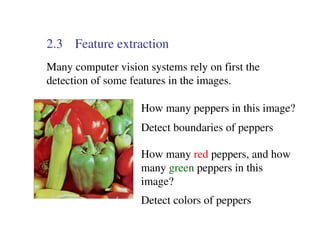
1. 2.3 Feature extraction
Many computer vision systems rely on first the
detection of some features in the images.
How many peppers in this image?
Detect boundaries of peppers
How many red peppers, and how
many green peppers in this
image?
Detect colors of peppers
2. 2.3.1 Edge detection
Edges are pixels at or around which the image
values undergo a sharp variation.
However, noise can also cause intensity variations.
A good edge detector should suppress image noise,
enhance and locate true edge pixels.
3. Types of edge
step edge ramp edge
line edge roof edge
Real edge may have multiple types superimposed with
noise, e.g. ramp + line + noise.
4. Edge descriptor – result of edge detection
edge direction edge normal
edge position - coordinates
edge direction - vector
edge normal - vector
edge strength – numeric value
5. Edge detection methods usually rely on calculations
of the first or second derivative along the intensity
profile.
I edge pixel
local peak
I’
I”
zero crossing
6. First derivative operator
∂I
G x ∂x
Calculate image gradient G (I( x, y)) = = ∂I
G y
∂y
magnitude G (I( x, y)) = G 2 + G 2
x y
approximation
G ( I( x , y)) = G x + G y or G ( I( x , y)) = max( G x , G y )
direction (with respect to x axis)
Gy
∠G (I( x, y)) = tan
−1
G
x
Threshold the gradient magnitudes to locate edges.
7. Discrete approximation
G x ≅ I[i, j + 1] − I[i, j] Gx = -1 1 Gy = 1 1
G y ≅ I[i, j] − I[i + 1, j] -1 1 -1 -1
convolution masks
The gradient is measured
1 1
at coordinates i + , j +
2 2
8. To avoid having the gradient calculated about an
interpolated point between pixels, you can use a 3 x 3
neighborhood, e.g. Sobel edge detector.
magnitude S(I( x, y)) = S 2 + S 2
x y
Sx = -1 0 1 Sy = 1 2 1
-2 0 2 0 0 0
-1 0 1 -1 -2 -1
convolution masks
The gradient is
measured at coordinates [i, j]
9. function sobeled(t)
% to perform Sobel edge detection
% threshold is t
[f_name, f_path] = uigetfile('*.bmp', 'Select an input image');
in_name = [f_path, f_name];
image = imread(in_name);
[height, width] = size(image);
imshow(image)
h = fspecial('sobel');
sx = imfilter(image, h); calculate Sx
v = h';
sy = imfilter(image, v); calculate Sy
for i = 1:height
for j = 1:width
mag(i,j)=sqrt(double(sx(i,j))^2+double(sy(i,j))^2); calculate magnitude
if mag(i,j) > t
sedimage(i,j) = 255;
else thresholding
sedimage(i,j) = 0;
end
end
end
figure
imshow(sedimage)
% save edge detection result
out_name = [f_path, 'sed_', f_name];
imwrite(sedimage, out_name, 'BMP');
end
10. Original Threshold = 100
Do you see any defects in the Sobel edge
detection result?
11. The errors in edge detection are false edges (false
positive FP) and missing edges (false negative FN).
Can you design other Sobel convolution masks for
measuring gradient in other directions?
12. Second derivative operator
The zero crossings can be
∂ 2I ∂ 2I
located by the Laplacian ∇ 2 I( x, y) = 2 + 2
∂x ∂y
operator
Discrete approximation
2
∇2 ≈ 0 1 0
∂ I
2
= I[i, j + 1] − 2I[i, j] + I[i, j − 1]
∂x 1 -4 1
∂ 2I
2
= I[i + 1, j] − 2I[i, j] + I[i − 1, j] 0 1 0
∂y
convolution mask
14. Edge operator involving two derivatives is affected by
noise more than an operator involving a single
derivative.
A better approach is to combine Gaussian filtering with
the second derivative – Laplacian of Gaussian (LoG).
• filter out the image noise using Gaussian filter
• enhance the edge pixels using 2D Laplacian
operator
• edge is detected when there is a zero crossing in
the second derivative with a corresponding large
peak in the first derivative
• estimate the edge location with sub-pixel
resolution using linear interpolation
15. Original 5 x 5 LoG mask, σ = 0.5
LoG edge detector can be implemented using the
MATLAB function edge.
16. An edge detector can reduce noise by smoothing the
image, but this will result in spreading of edges and
add uncertainty to the location of edge.
original image
I
Gaussian smoothed image
threshold
I’ edge detection result
I
”
thick edge
An edge detector can have greater sensitivity to the
presence of edges, but this will also increase the
sensitivity of the detector to noise.
17. The best compromise between noise immunity and
edge localization is the first derivative of a Gaussian –
e.g. Canny edge detector.
• edge enhancement
• non-maximum suppression
• hysteresis thresholding
18. edge enhancement:
Apply Gaussian smoothing to the image.
S[i, j] = G[i, j; σ] ∗ I[i, j]
G is a Gaussian with zero mean and standard deviation σ
Compute the gradient of the smoothed image and
estimate the magnitude and orientation of the gradient.
(S[i, j + 1] − S[i, j] + S[i + 1, j + 1] − S[i + 1, j])
P[i, j] =
2 M[i, j] = P[i, j] 2 + Q[i, j] 2
(S[i, j] − S[i + 1, j] + S[i, j + 1] − S[i + 1, j + 1])
Q[i, j] =
2 Q[i, j]
θ[i, j] = tan
P[i, j]
−1
19. non-maximum suppression:
M[i, j] may contain wide ridges around the local
maximum. This step is to thin such ridges to produce 1-
pixel wide edges. Values of M[i, j] along the edge
normal that are not peak will be suppressed.
Quantize edge normal orientations into 4, e.g. 0°, 45°,
90°, and 135° with respect to the horizontal axis. For
each pixel (i, j), find the orientation which best
approximates θ[i, j].
If M[i, j] is smaller than at least one of its two neighbors
along the quantized orientation, set M’[i, j] to zero.
Otherwise M’[i, j] = M[i, j].
20. hysteresis thresholding:
M’[i, j], after the non-maximum suppression step, may
still contain local maxima created by noise. To get rid of
false edges by thresholding, some false edges may still
remain if the threshold value is set too low, or some true
edges may be deleted if the threshold value is set too
high.
An effective scheme is to use 2 thresholds τl and τh,
e.g. τh = 2τl.
21. Scan the non-zero points of M’[i, j] in a fixed order.
If M’[i, j] is larger than τh, locate it as an edge pixel.
Else if any 8-neighbors of (i, j) have gradient
magnitude larger than τl, locate them as edge pixels.
Continue until another edge pixel is located by τh.
22. Original Thresholds [0.06 0.15], σ = 0.5
Canny edge detector can be implemented using the
MATLAB function edge.
23. 2.3.2 Corner detection
Corners are quite stable across sequences of images.
They are interesting features that can be employed for
tracking objects across sequences of images.
24. Consider an image point p, a neighborhood Q of p, and
a matrix C defined as
∑G2x ∑G G x y
C= Q
∑ G G
Q
Q x y ∑G 2
y
Q
We can think of C as a diagonal matrix
λ 1 0
C=
0 λ2
25. The two eigenvalues λ1 and λ2 are non-negative. A
corner is located in Q where λ1 ≥ λ2 > 0 and λ2 is
large enough.
• compute the image gradient
• for each image point p, form matrix C over a
neighborhood Q of p, compute the smaller
eigenvalue λ2 of C, if λ2 > threshold τ save the
coordinates of p into a list L
• sort L in decreasing order of λ2
• scan L from top to bottom, for each corner point p,
delete neighboring corner points in L