This document discusses the meaning of ethics. It begins by providing examples of how some business people defined ethics as following feelings, religious beliefs, laws, or social standards. However, the document argues that ethics cannot be reduced to any of these things. Ethics refers to well-founded standards of right and wrong that prescribe human obligations and duties, taking into account factors like rights, fairness, benefits to society, and virtues. True ethics can deviate from feelings, laws, religions or social acceptance at a given time.

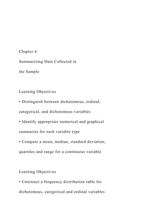
1. Chapter 4
Summarizing Data Collected in
the Sample
Learning Objectives
• Distinguish between dichotomous, ordinal,
categorical, and dichotomous variables
• Identify appropriate numerical and graphical
summaries for each variable type
• Compute a mean, median, standard deviation,
quartiles and range for a continuous variable
Learning Objectives
• Construct a frequency distribution table for
dichotomous, categorical and ordinal variables

2. • Provide an example of when the mean is a
better measure of location than the median
• Interpret the standard deviation of a continuous
variable
Learning Objectives
• Generate and interpret a box plot for a
continuous variable
• Produce and interpret side-by-side box plots
• Differentiate between a histogram and a bar
chart
Variable Types
• Dichotomous variables have 2 possible responses
(e.g., Yes/No)
• Ordinal and categorical variables have more than two
responses and responses are ordered and unordered,
respectively

3. • Continuous (or measurement) variables assume in
theory any values between a theoretical minimum and
maximum
Biostatistics
Two Areas of Applied Biostatistics:
Descriptive Statistics
– Summarize a sample selected from a population
Inferential Statistics
– Make inferences about population parameters
based on sample statistics.
Vocabulary
• Data elements/data points
• Subjects/units of measurement
• Population Vs. Sample
Sample vs Population
• Any summary measure computed on a sample

4. is a statistic
• Any summary measure computed on a
population is a parameter
n = sample size
N = population size
Example 4.1.
Dichotomous Variable
Frequency Distribution Table
Hypertension
Treatment
Frequency Relative
Frequency (%)
No 2313 65.5%
Yes 1219 34.5%
3532 100.0%
Relative Frequency Bar Chart for
Dichotomous Variable

5. Categorical Outcome
Sample: n=50
Population: Patients at health center
Variable: Marital status
Marital Status Number of Patients
Married 24
Separated 5
Divorced 8
Widowed 2
Never Married 11
Total 50
Categorical Outcome
Frequency Distribution Table
Marital Status Number of
Patients (f)
Relative

6. Frequency (f/n)
Married 24 0.48
Separated 5 0.10
Divorced 8 0.16
Widowed 2 0.04
Never Married 11 0.22
Total 50 1.00
Frequency Bar Chart
Ordinal Outcome
Sample: n=50
Population: Patients at health center
Variable: Self-reported current health status
Health Status Number of Patients
Excellent 19
Very Good 12
Good 9

7. Fair 6
Poor 4
Total 50
Ordinal Outcome
Frequency Distribution Table
Heath Status Freq. Rel. Freq. Cumulative
Freq
Cumulative
Rel. Freq.
Excellent 19 38% 19 38%
Very Good 12 24% 31 62%
Good 9 18% 40 80%
Fair 6 12% 46 92%
Poor 4 8% 50 100%
50 100%
Relative Frequency Histogram
0

8. 5
10
15
20
25
30
35
40
Poor Fair Good Very Good Excellent
Health Status
%
Example 4.2.
Ordinal Variable
Frequency Distribution Table
Blood Pressure
Categories
Frequency Relative Frequency
(%)

9. Normal 1206 34.1%
Pre-hypertension 1452 41.1%
Stage I hypertension 653 18.5%
Stage II hypertension 222 6.3%
Total 3533 100.0%
Relative Frequency Histogram for Ordinal
Variable
Continuous Variables
• Assume, in theory, any value between a
theoretical minimum and maximum
• Quantitative, measurement variables
Continuous Variable
• Population: Patients 50 years of age with
coronary artery disease
• Sample: n = 7 patients

10. • Outcome: Systolic blood pressure (mmHg)
Continuous Variable
Sample data
X
100
110
114
121
130
130
160
Continuous Variable
6.123
7
865
n
X

11. X
100
110
114
121
130
130
160
865
n
X
X mean Sample
Continuous Variable
Consider a second sample from the same population.

12. We record SBP on each subject in the second sample:
120 121 122 124 125 126 127
n = 7
= 865 / 7 = 123.6.
What is different between the 2 samples?
X
Continuous Variable
• Dispersion
X (X- )
100 -23.6
110 -13.6
114 -9.6
121 -2.6
130 6.4
130 6.4
160 36.4
865 0
X

13. Continuous Variable
• Dispersion
X (X- )
100 -23.6
110 -13.6
114 -9.6
121 -2.6
130 6.4
130 6.4
160 36.4
865 0
X
Mean Absolute Deviation (MAD):
n
| X - X| Σ
= MAD
Continuous Variable

14. X X
1n
)XΣ(X
s
2
2
374.6
6
2247.72
s
2
Sample Variance:
X (X- ) (X- )2
100 -23.6 556.96
110 -13.6 184.96
114 -9.6 92.16
121 -2.6 6.76

15. 130 6.4 40.96
130 6.4 40.96
160 36.4 1324.96
865 0 2247.72
Continuous Variable
• Sample Standard Deviation:
s = s
2
Standard Summary: n=7, X = 123.6, s=19.4
Median
Median
100 110 114 121 130 130 160
Median holds 50% of values above and
50% of values below
Order data
For n odd – median is middle value
For n even – median is mean of 2

16. middle values
Quartiles
Q1 = first quartile holds approximately 25% of the
scores at or below it and
Q3 = third quartile holds approx. 25% of the
scores at or above it
Q2 = ??
Continuous Variable
Median
Order data
100 110 114 121 130 130 160
Q1 Q3
Box and Whisker Plot
100 110 120 130 140 150 160
Min Q1 Median Q3 Max

17. Comparing Samples with
Box and Whisker Plots
100 110 120 130 140 150 160
Summarizing Location and Variability
• When there are no outliers, the sample mean
and standard deviation summarize location
and variability
• When there are outliers, the median and
interquartile range (IQR) summarize location
and variability, where IQR = Q3-Q1
Example
Sample: n=51 participants in a study of
cardiovascular risk factors.
Variable: age (years)
60 62 63 64 64 65 65 65 65 65 65

18. 66 66 66 66 66 67 67 67 68 68 68
70 70 70 71 71 72 72 73 73 73 73
73 73 75 75 75 76 76 77 77 77 77
77 79 82 83 85 85 87
Example
Sample mean:
71.3 =
51
3637
=
n
XΣ
= X
Sample variance:
41.4 =
50
/51)(3637 - 261,439
=
1 -n

19. /n)X(Σ - XΣ
= s
222
2
Sample standard deviation:
6.4 = 41.4 = s
Standard Summary: n=51, X = 71.3, s=6.4
Outliers
IQR = Interquartile Range = Q3 - Q1
= range of middle half of the data
Outliers are values which either:
exceed Q3 + 1.5 IQR, or
fall below Q1 - 1.5 IQR
Or outliers are outside + 3s X
Check for Outliers in Example
• Q1=66, Q3=76, IQR=10
– Lower=66-1.5(10)=51

20. – Upper=76+1.5(10)=91
• + 3s = 52.1 to 90.5X
Presenting Data
• Suppose we collapse ages into 5 mutually exclusive and
exhaustive categories:
Age Class Number of Individuals (freq.)
60-64 5
65-69 17
70-74 12
75-79 12
80-84 2
85-89 3
Presenting Data
Cumulative
Age Class Freq Rel Freq Freq Rel Freq
60-64 5 0.10 5 0.10

21. 65-69 17 0.33 22 0.43
70-74 12 0.24 34 0.67
75-79 12 0.24 46 0.91
80-84 2 0.04 48 0.95
85-89 3 0.06 51 1.00
Total 51 1.00
Frequency Histogram
0
2
4
6
8
10
12
14
16
18
60-
64
65-
69

22. 70-
74
75-
79
80-
84
85-
89
Age Class
F
r
e
q
u
e
n
c
y
Example 4.3.
Summarizing Continuous Variables

23. Diastolic blood pressures in n=10 randomly
selected participants attending the seventh
examination of the Framingham Offspring
Study
76 64 62 81 70
72 81 63 67 77
Summarizing Location
• What is a typical diastolic blood pressure?
Sample Mean
= Sum of diastolic blood pressures/n
= 713/10 = 71.3
Notation
• Let X represent the outcome of interest (e.g.,
X=diastolic blood pressure)
n
X

24. X mean Sample
Summarizing Variability
• Sample range
= maximum–minimum=81–62 = 19
• Sample variance
1n
)x(x
s
2
2
Sample Variance
DBP Deviation from Mean

25. 76 (76 - 71.3) = 4.7
64 (64 - 71.3) = -7.3
62 (62 - 71.3) = -9.3
81 9.7
70 -1.3
72 0.7
81 9.7
63 -8.3
67 -4.3
77 5.7
S X = 71.3 S Deviations from Mean = 0
Sample Variance
DBP Deviation from Mean Squared Deviations
76 (76 - 71.3) = 4.7 22.09
64 (64 - 71.3) = -7.3 53.29
62 (62 - 71.3) = -9.3 86.49
81 9.7 94.09

26. 70 -1.3 1.69
72 0.7 0.49
81 9.7 94.09
63 -8.3 68.89
67 -4.3 18.49
77 5.7 32.49
S X = 71.3 S Deviations = 0 S Deviations2 = 472.10
Sample Variance and Sample Standard
Deviation
46.52
9
10.472
1n
)x(x
s
2
2

27. 2.746.52
1n
)x(x
s
2
Median
• Median holds 50% of values above and 50%
of values below
– Order data
– For n odd – median is middle value
– For n even – median is mean of 2 middle values

28. Median = 71
62 63 64 64 70 | 72 76 77 81 81
Quartiles
• Q1 = first quartile = holds 25% of values
below it
• Q3 = third quartile = holds 25% of values
above it
Median = 71
62 63 64 64 70 | 72 76 77 81 81
Q1 Q3
Determining Outliers
• Outliers are values
below Q1-1.5(Q3-Q1) or
above Q3+1.5(Q3-Q1)
• In Example 4.3,
lower limit = 64-1.5(77-64) = 44.5

29. and upper limit=77+1.5(77-64) = 96.5
• Outliers?
• Mean or Median? s or IQR?
Box Plot for Continuous Variable
60
65
70
75
80
d
b
p
Numerical and Graphical Summaries
• Dichotomous and categorical
– Frequencies and relative frequencies
– Bar charts (freq. or relative freq.)
• Ordinal

30. – Frequencies, relative frequencies, cumulative
frequencies and cumulative relative frequencies
– Histograms (freq. or relative freq.)
Numerical and Graphical Summaries
• Continuous
– Mean, standard deviation, minimum, maximum,
range, median, quartiles, interquartile range
– Box plot
What is Ethics?
Manuel Velasquez, Claire Andre, Thomas Shanks, S.J., and
Michael J. Meyer
Some years ago, sociologist Raymond Baumhart asked business
people, "What does
ethics mean to you?" Among their replies were the following:
"Ethics has to do with what my feelings tell me is right or
wrong."
"Ethics has to do with my religious beliefs."
"Being ethical is doing what the law requires."

31. "Ethics consists of the standards of behavior our society
accepts."
"I don't know what the word means."
These replies might be typical of our own. The meaning of
"ethics" is hard to pin down,
and the views many people have about ethics are shaky.
Like Baumhart's first respondent, many people tend to equate
ethics with their feelings.
But being ethical is clearly not a matter of following one's
feelings. A person following
his or her feelings may recoil from doing what is right. In fact,
feelings frequently deviate
from what is ethical.
Nor should one identify ethics with religion. Most religions, of
course, advocate high
ethical standards. Yet if ethics were confined to religion, then
ethics would apply only to
religious people. But ethics applies as much to the behavior of
the atheist as to that of the
devout religious person. Religion can set high ethical standards
and can provide intense
motivations for ethical behavior. Ethics, however, cannot be
confined to religion nor is it
the same as religion.
Being ethical is also not the same as following the law. The law
often incorporates ethical
standards to which most citizens subscribe. But laws, like
feelings, can deviate from what
is ethical.
Finally, being ethical is not the same as doing "whatever society

32. accepts." In any society,
most people accept standards that are, in fact, ethical. But
standards of behavior in
society can deviate from what is ethical. An entire society can
become ethically corrupt.
Nazi Germany is a good example of a morally corrupt society.
Moreover, if being ethical were doing "whatever society
accepts," then to find out what is
ethical, one would have to find out what society accepts. To
decide what I should think
1
about abortion, for example, I would have to take a survey of
American society and then
conform my beliefs to whatever society accepts. But no one
ever tries to decide an ethical
issue by doing a survey. Further, the lack of social consensus on
many issues makes it
impossible to equate ethics with whatever society accepts. Some
people accept abortion
but many others do not. If being ethical were doing whatever
society accepts, one would
have to find an agreement on issues which does not, in fact,
exist.
What, then, is ethics? Ethics is two things. First, ethics refers to
well-founded standards
of right and wrong that prescribe what humans ought to do,
usually in terms of rights,
obligations, benefits to society, fairness, or specific virtues.
Ethics, for example, refers to
those standards that impose the reasonable obligations to refrain

33. from rape, stealing,
murder, assault, slander, and fraud. Ethical standards also
include those that enjoin
virtues of honesty, compassion, and loyalty. And, ethical
standards include standards
relating to rights, such as the right to life, the right to freedom
from injury, and the right
to privacy. Such standards are adequate standards of ethics
because they are supported by
consistent and well-founded reasons.
Secondly, ethics refers to the study and development of one's
ethical standards. As
mentioned above, feelings, laws, and social norms can deviate
from what is ethical. So it
is necessary to constantly examine one's standards to ensure
that they are reasonable and
well-founded. Ethics also means, then, the continuous effort of
studying our own moral
beliefs and our moral conduct, and striving to ensure that we,
and the institutions we help
to shape, live up to standards that are reasonable and solidly-
based.
This article appeared originally in Issues in Ethics IIE V1 N1
(Fall 1987). Revised in
2010.
2
What is Ethics?Manuel Velasquez, Claire Andre, Thomas
Shanks, S.J., and Michael J. Meyer

34. Chapter 3
Quantifying the Extent of Disease
Critical Components of RCT
• Randomization
• Control Group – Ethical Issues
• Monitoring
– Interim Analysis
– Data and Safety Monitoring Board
• Data Management
• Reporting
Learning Objectives
• Define and differentiate prevalence and
incidence
• Select, compute and interpret the appropriate
measure to compare the extent of disease
between groups

35. • Compare and contrast, compute and interpret
relative risks, risk differences, and odds ratios
Prevalence
• Proportion of participants with disease at a particular
point in time
baselineatexaminedpersonsofNumber
diseasewithpersonsofNumber
Example 3.1.
Computing Prevalence
Free of
CVD
History of
CVD
Total
Men 1548 244 1792
Women 1872 135 2007

36. Total 3420 379 3799
Prevalence of CVD = 379/3799 = 0.0998 = 9.98%
Prevalence of CVD in Men = 244/1792 = 0.1362 = 13.62%
Prevalence of CVD in Women = 135/2007 = 0.0673 = 6.73%
Example-H1N1 Outbreak
• H1N1 outbreak first noticed in Mexico
• Large outbreak early on in La Gloria-a small village
outside of Mexico City.
• Studied extensively in the first report on H1N1 (Fraser,
Donelly et al. “Pandemic potential of a strain of Influenza
(H1N1): early
findings”, Science Express, 11 May 2009.)
• Important questions: Who is most likely to be
impacted? What are the characteristics of people
commonly impacted?
Computing Prevalence
Age No ILI ILI Total
<44 years 703 522 1225
> 44 years 256 94 350

37. Total 959 616 1575
Data on H1N1 outbreak in La Gloria, Mexico.
n=1575 villagers (out of 2155) were surveyed to
determine if they had influenza like illness (ILI)
between 2/15/09 and 4/27/09.
Computing Prevalence
Age No ILI ILI Total
<44 years 703 522 1225
> 44 years 256 94 350
Total 959 616 1575
Prevalence of ILI=616/1575=0.3911=39.11%
Prevalence of ILI in <44=522/1225=0.4261=42.61%
Prevalence of ILI in >44=94/350=0.2686=26.86%
Incidence
• Likelihood of developing disease among persons free of
disease who are at risk of developing disease

38. baselineatriskatpersonsofNumber
period specified a during diseasedevelop whopersonsofNumber
freediseasearepersonswhichduringtimeoflengthstheofSum
period specified a during diseasedevelop whopersonsofNumber
Rate Incidence
Computing Incidence
• Cumulative incidence requires complete
follow-up on all participants
• Person-time data is used to take full advantage
of available information in incidence rate
• Incidence rate often expressed as an integer
per multiple of participants over a specified
time
Incidence of CVD?
1 Disease-Free

39. 2 CVD
3 Death
4 Disease-Free
5 CVD
0 5 10 Yrs
Study Start
Incidence Rate
freediseasearepersonswhich
duringtimeoflengthstheofSum
period specified a during
diseasedevelop whopersonsofNumber
Rate Incidence
Incidence of CVD
Incidence = 2/(10+9+3+10+5) = 2/37

40. = 0.054
5.4 per 100 person-years
Example 3.2.
Computing Incidence
Develop
CVD
Total Follow-Up
Time (years)
Men 190 9984
Women 119 12153
Total 309 22137
Incidence Rate of CVD in Men = 190/9984 = 0.01903
= 190 per 10,000 person-years
Incidence Rate of CVD in Women = 119/12153 = 0.00979
= 98 per 10,000 person-years
Computing Incidence
Developed ILI Total Follow-Up Time (years)

41. <44 years 522 20,064
> 44 years 94 3,514
Total 616 23,578
Incidence Rate of ILI in <44 = 522/20064 = 0.0260
= 260 per 10,000 person-years
Incidence Rate of ILI in >44 = 94/3514 = 0.0268
= 268 per 10,000 person-years
Comparing Extent of Disease Between
Groups
• Risk difference (excess risk)
unexposedexposed
unexposedexposed
unexposedexposed
Rate IncidenceRate Incidence
Incidence CumulativeIncidence Cumulative
PrevalencePrevalence

42. Comparing Extent of Disease Between
Groups
• Risk difference of prevalent CVD in smokers versus
non-smokers
smokers-nonsmokers
Free of
CVD
History
of CVD
Total
Non-Smoker 2757 298 3055
Current Smoker 663 81 744
3420 379 3799
= 81/744 – 298/3055 = 0.1089 – 0.0975 = 0.0114
Population Attributable Risk of CVD in

43. Smokers vs Non-Smokers
overall
smokers-nonoverall
Prevalence
Free of
CVD
History
of CVD
Total
Non-Smoker 2757 298 3055
Current Smoker 663 81 744
3420 379 3799
= (0.0998 – 0.0975) / 0.0998 = 0.023 = 2.3%
Comparing Extent of Disease Between
Groups
• Risk difference of history of ILI in Males and Females in
La Gloria

44. MalesFemales
No ILI ILI Total
Males 517 260 777
Females 442 356 798
959 616 1575
= 356/798 - 260/777 = 0.4461 – 0.3346 = 0.1115
Comparing Extent of Disease Between
Groups
• Relative risk
unexposed
exposed
Prevalence
Prevalence
Comparing Extent of Disease Between
Groups

45. • Relative risk of CVD in smokers versus non-smokers
smokers-non
smokers
Prevalence
Prevalence
Free of
CVD
History
of CVD
Total
Non-Smoker 2757 298 3055
Current Smoker 663 81 744
3420 379 3799
= 0.1089/0.0975 = 1.12
Comparing Extent of Disease Between
Groups
• Relative risk of ILI in females versus males

46. males
females
Prevalence
Prevalence
No ILI ILI Total
Males 517 260 777
Females 442 356 798
959 616 1575
= 0.4461/0.3346 = 1.33
Comparing Extent of Disease Between
Groups
• Odds ratio
)Prevalence(1
Prevalence
)Prevalence(1
Prevalence
unexposed

47. unexposed
exposed
exposed
Comparing Extent of Disease Between
Groups
• Odds ratio of CVD in hypertensives versus non-
hypertensives
No
CVD
CVD Total
Non-hypertensive 2754 188 2942
Hypertensive 659 181 840
3413 369 3782
04.4
932.0/068.0

48. 725.0/275.0
)2942/881(1
188/2942
)840/181(1
181/840
Comparing Extent of Disease Between
Groups
• Odds ratio of ILI in younger group versus older group
Age No ILI ILI Total
<44 years 703 522 1225
> 44 years 256 94 350
Total 959 616 1575
02.2
731.0/269.0
574.0/426.0

49. )350/94(1
94/350
)1225/522(1
522/1225
Relative Risks and Odds Ratios
• Not possible to estimate relative risk in case-
control studies
• Can estimate odds ratio because of its
invariance property
Invariance Property of Odds Ratio
Cancer
(Case)
No Cancer
(control)

50. Total
Smoker 40 29 69
Non-smoker 10 21 31
50 50 100
Case-control study to assess association
between smoking and cancer
Invariance Property of Odds Ratio
Cancer
(Case)
No Cancer
(control)
Total
Smoker 40 29 69
Non-smoker 10 21 31
50 50 100
Odds ratio for cancer in smokers versus non-smokers
= (40/29) / (10/21) = 2.90
Odds of smoking in patients with cancer versus not

51. = (40/10) / (29/21) = 2.90!