Optical projection tomography (OPT) is a computed tomography technique used to image samples between 0.5-15mm in size. It involves taking 2D projections of a sample rotated over 360 degrees and computationally reconstructing the 3D structure. Standard reconstruction uses filtered backprojection which can produce streak and ring artifacts. Total variation minimization has been shown to improve reconstruction quality by smoothing small fluctuations while preserving edges. The document reviews various techniques for reducing artifacts in OPT reconstruction through additional projections, model-based iterative methods, and total variation minimization.

1. Microsc. Microanal., page 1 of 14
1 doi:10.1017/S1431927615015226
2
© MICROSCOPY SOCIETY OF AMERICA 2015
3 Total Variation-Based Reduction of Streak Artifacts,
4 Ring Artifacts and Noise in 3D Reconstruction from
5 Optical Projection Tomography
6 Jan Michálek*
7 Department of Biomathematics, Institute of Physiology of the Czech Academy of Sciences, Videnska 1083, 14220 Prague 4,
8 Czech Republic
9 Abstract: Optical projection tomography (OPT) is a computed tomography technique at optical frequencies for
10 samples of 0.5–15 mm in size, which fills an important “imaging gap” between confocal microscopy (for smaller
11 samples) and large-sample methods such as fluorescence molecular tomography or micro magnetic resonance
12 imaging. OPT operates in either fluorescence or transmission mode. Two-dimensional (2D) projections are taken
13 over 360° with a fixed rotational increment around the vertical axis. Standard 3D reconstruction from 2D OPT
14 uses the filtered backprojection (FBP) algorithm based on the Radon transform. FBP approximates the inverse
15 Radon transform using a ramp filter that spreads reconstructed pixels to neighbor pixels thus producing streak
16 and other types of artifacts, as well as noise. Artifacts increase the variation of grayscale values in the reconstructed
17 images. We present an algorithm that improves the quality of reconstruction even for a low number of projections
18 by simultaneously minimizing the sum of absolute brightness changes in the reconstructed volume (the total
19 variation) and the error between measured and reconstructed data. We demonstrate the efficiency of the method
20 on real biological data acquired on a dedicated OPT device.
21 Key words: optical projection tomography, microscopy, artifacts, total variation, data mismatch
22
23
INTRODUCTION
24 Optical projection tomography (OPT) is a recently (Sharpe
25 et al., 2002) developed implementation of computed tomo-
26 graphy (CT) techniques at optical frequencies. A series of
27 two-dimensional (2D) optical projections through a sample
28 are generated at varying orientations (Fig. 1) from which the
29 3D structure of the sample can be computationally recovered
30 (Bassi et al., 2011).
31 In transmission mode, a collimated light source is used
32 to transmit a parallel beam through the sample to acquire
33 projections at the desired wavelength. Images are recorded
34 on a CCD camera throughout a full 360° rotation. Using
35 computer software the original 3D information is subsequently
36 recalculated.
37 In fluorescence mode, optical tomography projections
38 can be obtained either by recording the autofluorescence
39 emitted by the tissue or by using fluorescent antibody labeled
40 specimens embedded in agarose and made semitransparent
41 in an organic solvent (typically a mixture of benzyl alcohol
42 and benzyl benzoate, BABB). The specimen is exposed to
43 appropriate excitation light and the emitted light is captured
44 from a number of angular positions on the CCD chip of
45 the camera.
46 OPT is suitable for many important model organisms,
47 e.g. insects, animal embryos, or small animal extremities,
48which are too large for techniques such as confocal imaging
49(CLSM), and too small for large-sample methods such as
50fluorescence molecular tomography, X-ray CT or micro
51magnetic resonance imaging (μMRI). OPT covers the range
52of sample sizes from about 0.5 to 15 mm, and thus fills the
53“imaging gap” between CLSM and μMRI. OPT allows
54acquisition of 3D data with proper morphological and spatial
55information without the need to cut the specimen and
56without deformations introduced by cutting. A disadvantage
57of OPT is that its resolution is inferior to that of CLSM
58(CLSM: ~200 nm/pixel; OPT: >2 µm/pixel).
59In 3D reconstruction from tomography projections, a
60slice through the specimen at some height z is reconstructed
61computationally from projections of the rotating specimen
62over a range of angles. The mathematical problem of
63reconstruction from a finite number of projections may be
64underdetermined: if we acquire, e.g., OPT projections from
65400 directions with 512 pixels in each projection, we get
66204,800 measured values. To reconstruct the slice, brightness
67in 512 × 512 = 262,144 pixels needs to be computed, i.e. we
68have 262,144 unknowns, but only 204,800 projected points
69to calculate from. If we represent the Radon transform in
70matrix form
R ´ u = b; (1)
71where R is the Radon projection matrix, b the known 204,800
72projection values (sinogram), and u the 262,144 unknown
73pixels, then the equation system is underdetermined and can
74be satisfied by infinitely many solutions u for the sought slice,*Corresponding author. michalek@biomed.cas.cz
Received April 30, 2015; accepted September 3, 2015

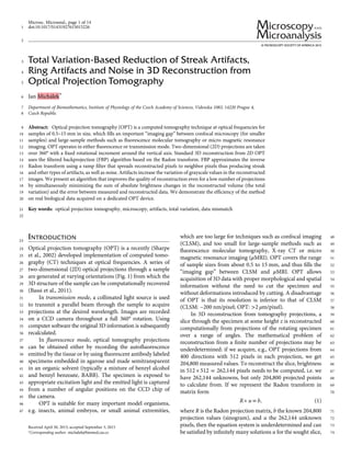
2. 75 many of which do not match the original. Mismatching areas
76 often exhibit conspicuous patterns called artifacts and are
77 visually unacceptable.
78 The standard method for 3D tomographic reconstruc-
79 tion from OPT series is the filtered backprojection (FBP)
80 algorithm, most widely used in other types of parallel beam
81 CT, e.g. X-ray CT. FBP is an approximation of the inverse
82 Radon transform, the theory of which was first published
83 in (Radon, 1917). The FBP tackles the problem of under-
84 determinacy of (1) by applying a ramp filter to acquired data
85 before backprojection. The ramp filter essentially substitutes
86 the missing data by spreading reconstructed pixel values over
87 neighbor points. In FBP-reconstructed images one can
88 notice artifacts, such as:
89 ∙ streak artifacts (Figs. 2e and 3e): fan-shaped streaks in the
90 direction of backprojection, centered at the axis of rotation
91 of the specimen and introduced by the ramp-filter
92 blurring;
93 ∙ ring artifacts centered at the rotation axis (Figs. 2e and 3e)
94 caused by miscalibrated detector elements and not specific
95 only to FBP;
96 ∙ noise (Fig. 3e) obviously does not correspond to any biological
97 structures of the specimen (also not specific to FBP).
98 Though theoretical papers on improving the quality of
99 tomography reconstructions are abundant, examples based
100 on genuine biological data are scarce. Efficacy is usually
101 demonstrated only for artificial, digitized or physical,
102 phantoms, satisfying idealized assumptions that seldom
103 hold for real biological data, such as sparsity (i.e., low
104 number of nonzero values) either of the image (most pixels
105 black) or of its gradient (most image areas are constant such
106 as the well-known Shepp–Logan phantom). In addition,
107 tomography projections are often computer-simulated
108 rather than acquired on a real CT scanner. Since our goal is
109 to reduce artifacts in real-life tomography reconstruction,
110 papers assuming some kind of sparsity or presenting only
111phantom reconstructions were not included in the following
112state-of-the-art review.
113Reports on reducing artifacts in tomography recon-
114structions from genuine biological data are relatively rare.
115Bruyant et al. (2000) proposed to generate additional
116projections by computational means to reduce the streak
117artifact. They introduced a postacquisition process called
118interpolation of projections by contouring, which creates
119new pseudoprojections by interpolating measured sinogram
120values on a new, denser, grid containing more angles or/and
121detector bins. In a clinical study, they found that increasing
122the number of angles by interpolation can reduce radial
123streaks, while when they interpolated between the bins the
124improvement was not conclusive.
125Yu et al. (2011) presented a model-based iterative
126reconstruction (MBIR) method using spatially non-
127homogeneous iterative coordinate descent (NH-ICD)
128optimization. MBIR algorithms work by first forming an
129objective function which incorporates an accurate system
130model, statistical noise model, and prior model. The image is
131then reconstructed by computing an estimate that minimizes
132the resulting objective function. They consider the image
133and the data as random vectors, and the goal is to reconstruct
134the image by computing the maximum a posteriori
135estimate using a Taylor series expansion to approximate the
136log-likelihood term by a quadratic function. Voxels of
137the image are updated in a spatially NH-ICD to accelerate
138convergence. In order to speed up convergence, the order of
139voxel updates is determined by a voxel selection criterion
140related to the absolute sum of the update magnitudes at the
141last visit. They compared axial slices reconstructed from a
142512 × 512 abdomen scan using FBP and their MBIR NH-ICB
143algorithm. Some of the streak artifacts in the FBP recon-
144struction were no longer visible in the ICB reconstruction.
145When CT projections are acquired at a small number of
146views, the system may become severely underdetermined,
147and analytic methods such as FBP may yield reconstructions
148with considerable aliasing artifacts such as sharp streaks.
149Moreover, data measured in real experiments are con-
150taminated by various physical factors such as noise and
151scatter, and thus they may contain components that are
152inconsistent with the discrete imaging model. Han
153et al. (2011) investigated low-dose micro-CT and its
154application to specimen imaging from substantially reduced
155projection data by using an algorithm referred to
156as the adaptive-steepest-descent-projection-onto-convex-sets
157(ASD-POCS) which reconstructs an image through mini-
158mizing the total variation (TV) of the image and enforcing
159data constraints. The ASD-POCS algorithm minimizes the
160TV of the estimated image subject to data condition and
161nonnegativity constraints:
u* = arg min uk kTV s:t: Ru - bk k2 ≤ ε and u ≥ 0;
162where uk kTV, referred to as the image TV, denotes the norm
163of the discrete gradient magnitude of the image, and
164Ru - bk k2 indicates the Euclidean distance between measured
165data and data estimated from the reconstructed image.
Figure 1. Photograph of an optical projection tomography
system built by Politecnico di Milano (Dipartimento di Fisica) for
imaging cleared tissue samples. Telecentric optics is used in order
to keep constant magnification throughout the specimen. The
white LED is used for transmission optical projection tomography
(OPT). Alternatively, the 470 nm LED can be used as excitation
light source for the fluorescence OPT.
2 Jan Michálek

3. 166 A tolerance parameter ε is introduced to relax the requirement
167 on data distance. The ASD-POCS iterations alternatingly
168 employ the steepest descent (SD) for minimizing the image
169 TV, and POCS methods for minimizing the data distance.
170 Both minimizations are carried out with respect to the sought
171 image u. Both SD and POCS steps are followed by a nonlinear
172 projection operation that enforces the positivity constraint by
173 setting all negative image voxels to zero. Comparison of the
174 ASD-POCS, FDK (Feldkamp, Davis, and Kress algorithm)
175 and POCS (without TV) reconstruction methods applied to CT
176 projections of a porcine heart and kidney specimens suggests
177 that the ASD-POCS algorithm can effectively suppress streak
178 artifacts and noise that were observed in tomography slices
179 reconstructed with FDK and POCS algorithms.
180 Park et al. (2012) proposed a low-dose cone-beam CT
181 using a minimal number of noisy projections. Tomography
182 reconstruction is obtained as the result of constrained
183 minimization with respect to u of the function
f ðuÞ = TVðuÞ + λ Ru - bk k2
2 s:t: u ≥ 0:
184 Minimization is done in the gradient direction, but with a
185 special choice of the step size. They use an approximate
186second-order solver, proposed by Barzilai and Borwein. In
187their GP-BB approach, the step size is chosen based on both
188the current and the previous gradient which could result in a
189nonmonotonic, but faster, convergence. For 364 projections
190with 1,024 bins, their algorithm takes about 234 s when
191implemented on a graphic processing unit (GPU). The
192authors report that minimizing the TV-enhanced problem
193results in a visually better quality image than that of the FDK
194(i.e., less noise, streaking artifacts around bones, etc.).
195Leary et al. (2013) have followed a Fourier-based
196approach to electron tomography (ET) reconstruction.
197They found that, for application to ET data sets, where the
198aim is to reconstruct the 3D density of the sample and the
199sample is expected to be approximately piecewise constant,
200simultaneous enforcement of sparsity in both the image and
201gradient domains yields the highest fidelity reconstructions.
202They minimize the weighted sum
f ðuÞ = λTVTVðuÞ + λl uk k1 + λ Φu - bk k2
2
Φ::sensing matrix;
203between the data fidelity term and the sparsity term which is
204a blend of TV and nonzero image values evaluated by uk k1.
Figure 2. a–d: Four out of 400 optical projection tomography projections from different angles of a muscle specimen
of a young pig with nerve fascicles (n. medianus); benzyl alcohol/benzyl benzoate clearing, acquired in transmission
mode on our “Milano” scanner with 400 projections 1,004 × 1,002 pixels in size, (e) FBP reconstruction from 400
projections exhibits streak and ring artifacts. Concentric fan-shaped streaks are caused by the way filtered back-
projection (FBP) approximates the Radon transform, and by having less measured data than pixels to be reconstructed
(400 projections × 1,004 pixels = 401,600 measured values to reconstruct 710 × 710 = 504,100 pixels of the slice). The
arrowhead points to the most pronounced ring artifact. Ring artifacts around the center of rotation can be caused by
miscalibrated detector elements or by misalignment between the true axis of rotation during data acquisition, and the
axis assumed by the reconstruction algorithm, (f) total variation (TV) reconstruction from 400 projections.
Reconstruction in Optical Projection Tomography 3

4. 205 They first Fourier transform the projection images to obtain
206 radial samples of the object in the Fourier domain. This data is
207 then Fourier transformed into the image domain using the
208 nonuniform fast Fourier transform (NUFFT). In conjunction
209 with the NUFFT, for the sparsity-seeking optimization process
210 they have used a conjugate gradient descent algorithm.
211 Niu et al. (2014) start likewise from the TV minimiza-
212 tion framework with a data fidelity constraint
u* = arg min uk kTV s:t: 0:5 Ru - bk k2
2 ≤ ε and u ≥ 0;
213 and convert this formulation into minimization of the loga-
214 rithmic barrier function
u* = arg min uk kTV - logðε - 0:5 Ru - bk k2
2
ÁÂ Ã
s:t:u ≥ 0:
215 Here, the vector b represents the line integral measurements
216 (i.e., after the logarithmic operation on the raw projections),
217 R is the system matrix modeling the forward projection,
218 u the vectorized patient image to be reconstructed, Ru - bk k2
2
219 calculates the L2
norm in the projection space, and uk kTV the
220 TV term defined as the L1
norm of the spatial gradient
221 image. The user-defined parameter ε is an estimate of total
222 measurement errors. The authors propose to minimize the
223 logarithmic barrier function using gradient-based algorithms.
224 The reconstructed images have a size of 512×512 pixels. For
225 tomography reconstruction of one slice from a head-and-neck
226 patient study, Niu et al. (2014) report significant reduction
227of the artifacts from few-view reconstruction using their new
228method in comparison to standard FBP reconstruction.
229The reason why TV minimization is efficient in reducing
230artifacts is that it enforces smoothing of small fluctuations in
231reconstructed slices, yet a large sudden change in image
232brightness is not penalized more than a slow continuous
233brightness change. Thus, small variations like streaks or ring
234artifacts are smoothed, but sharp edges in the specimen remain
235untouched. Figure 4 illustrates this property.
236
MATERIALS AND METHODS
237Tomography Reconstruction through Minimization
238of a Weighted Sum of TV and the Data Mismatch
239Methods of artifact reduction due to Han et al. (2011) and
240Niu et al. (2014) minimize the TV of the reconstructed image
u* = arg min uk kTV;
241under the relaxed constraint on the data fidelity
0:5 Au - bk k2
2 ≤ ε;
242and constraints on data positiveness
u ≥ 0:
243Such constrained minimization of the TV yields excellent
244tomography reconstruction in cases where the magnitude of the
image gradient is nonzero only in a very low number of
Figure 3. a–d: Sample optical projection tomography (OPT) projections from four different angles of a 3 × 3 × 3 mm3
block of a rat brain stained in vivo by biotinylated Lycopersicon esculentum (tomato lectin), and cleared using the
benzyl alcohol/benzyl benzoate protocol. Data acquisition was done on a commercial OPT scanner Bioptonics 3001
with projections 512 × 512 pixels in size, in fluorescence mode with excitation wavelength 425/40 nm (band pass), and
emission wavelength from 475 nm (high pass), (e) noise and ring artifacts in filtered backprojection (FBP) reconstruc-
tion from 400 projections, the arrowhead points to the center of the rings, (f) total variation (TV) reconstruction from
400 projections removes the noise-like texture from the reconstruction and brings forward fine details that were hidden
by the artifacts in the FBP reconstruction.
4 Jan Michálek

5. 245 locations, i.e. is sparse in the terminology of compressed sensing
246 (Candès et al., 2006). Sparsity of the gradient means that the
247 image consists of large regions with constant grayscale values.
248 The well-known Shepp–Logan phantom in Figure 5a is a
249 typical example of a synthetic tomography specimen with
250 sparse gradient.
251 We developed our own algorithm for tomography
252 reconstruction by constrained TV minimization, and tested
253 it using software projections of the 512 × 512 Shepp–Logan
254 phantom. The projections were taken between 0° and 180°
255 with an angle increment of 2°. This yielded 91 projections
256 with 724 bins each, which totals to 724 × 91 = 65,884 known
257 data points. Tomography reconstruction had to recover
258 512 × 512 = 262,144 unknown pixels, i.e. we had only
259 25.133% of the data needed to solve uniquely the underlying
260 equations. Since the Shepp–Logan phantom is piecewise
261 constant, its gradient is sparse, and the constrained TV-
262 based reconstruction (Fig. 5b) matches almost perfectly the
263 original, confirmed also by the profile in Figure 5f. FBP
264reconstruction contains many artifacts (Figs. 5c–5g).
265A justified question arises if the same artifact reduction as
266with TV could be achieved by low-pass filtering of the
267FBP-reconstructed slice, which is much faster than TV
268minimization. The answer is it could not: Figures 5d and 5h
269show the result of FBP filtered with a 10 × 10 pixel Gaussian
270filter with σ = 3. Streaks are visibly reduced, but sharp
271transitions between regions of constant intensity have been
272smeared. This confirms that TV-enhanced tomography
273reconstruction preserves sharp edges, while low-pass filter-
274ing of the reconstructed image does not, even though it also
275reduces the artifacts to some extent.
276The assumption of gradient sparsity rarely holds true for
277biological specimens. We attempted constrained TV-based
278reconstruction from projections of biological tissue with
279slowly varying optical density, i.e. with large areas of nonzero
280gradient. Constrained TV-based reconstruction yielded
281implausible images with watercolor-like large patches of
282constant brightness. Therefore, we decided to replace TV
total
variation
total
variation
a b
Figure 4. Total variation does not penalize discontinuities. Example of a discontinuous and a continuous function
whose total variation is the same: (a) discontinuous function and its total variation, (b) continuous function and its
total variation.
Figure 5. Tomography reconstruction from 91 projections of the 512 × 512 Shepp–Logan phantom. Upper row: (a) the
phantom, (b) constrained total variation reconstruction, (c) classical filtered backprojection (FBP) reconstruction,
(d) low-pass filtered FBP reconstruction, 10 × 10 pixel Gaussian filter with σ = 3. Lower row: (e–h) brightness profiles
along the central horizontal line in the images of the first row.
Reconstruction in Optical Projection Tomography 5

6. 283 minimization under the constraint of a perfect data match
284 with the minimization of a weighted sum of TV and the data
285 mismatch. In the minimization of a weighted sum of TV and
286 the data mismatch, our aim is to find a reconstructed image
287 ur which minimizes the function
FðuÞ = TVðuÞ +
μ
2
Ru - bk k2
2;
288 i.e.
ur = arg min
u
TVðuÞ +
μ
2
Ru - bk k2
2
|fflfflfflfflffl{zfflfflfflfflffl}
L2
2
6
4
3
7
5: (3)
289 This problem statement differs from that of Park et al.
290 (2012) only in the absence of the constraint u ≥ 0. However,
291 since Niu et al. (2014) report stability problems of the
292 Barzilai–Borwein gradient algorithm used by Park et al.
293 (2012), we developed our own algorithm based on variable
294 splitting and alternating direction method of multipliers
295 (ADMM) for the minimization in (3). In the following,
296 we will use the shorthand TV-L2
for this algorithm. The
297 algorithm is different from all algorithms reviewed in this
298 subsection.
299 The Algorithm
300 The algorithm is derived in the Appendix. We present here
301 only the resulting steps. The meaning of the math symbols is
302 explained in Table 1.
303 Using the procedure of variable splitting described in the
304 Appendix, the minimization of the total-variation regular-
305 ized mismatch between the measured projections and
306 reprojected tomography slices in (3) can be replaced by
307 the minimization of the augmented Lagrangian, in which
308 the function
LAðw; uÞ = wk k1 +
β
2
Du - w - ck k2
2 +
μ
2
Ru - bk k2
2;
309 is minimized iteratively by alternating minimizations with
310 respect to u and w (ADMM). The algorithm operates in three
311 phases:
312 Step 1. Keeping w, c constant, do one optimal descent step in
313 the gradient direction of LA(w, u)
314 ∙ gradient: gk
= βDT
(Duk
− wk
− ck
) + μRT
(Ruk
− b)
315 ∙ optimum step size: αk
= (gkT
gk
)/(gkT
Agk
), where
316 A = βDT
D + μRT
R
317 ∙ SD step: uk + 1
= uk
− αk
gk
318 Step 2. Keeping u, c constant minimize LA(w, u) with respect
319 to w:
320 ∙ min
w
LAðw; uk + 1
Þ )wk + 1
p = max Dpuk + 1
- ck
p
- 1
β
;0
n o
321 ´ sgn Dpuk + 1
- ck
p
for all pixels p, where all the operations
322 are done componentwise
323 Step 3. Update the vector of Lagrangian multipliers c:
324 ∙ ck + 1
= ck
− (Duk + 1
− wk + 1
)
325 until a termination criterion is satisfied.
326Relationship between our Method and the
327Compressed Sensing Approach
328In its pure form, image reconstruction based on compressive
329sensing assumes that there exists a representation of
330the image in form of a linear combination of some basis
331functions such that the number of the basis functions needed
332to represent the image is much lower than the number of
333pixels of the image (Candès and Wakin, 2008; Romberg,
3342008). The image is reconstructed so as to minimize the
335number of needed basis elements under the constraint of
336data fidelity, which in case of computer tomography means
337that Radon reprojection of the reconstructed image matches
338the measured Radon projections. This is the approach
Table 1. List of Math Symbols.
F(u) Weighted sum of total variation and the data
mismatch
TV Total variation
u The unknown image (a slice in the three-dimensional
volume) to be reconstructed (N-vector)
ur Minimizer of F(u) (the reconstructed slice)
R Radon projection matrix
μ/2 Weight of the data mismatch term
b Measured values of parallel Radon tomography
projections
ν 2N-vector of Lagrange multipliers
c 2N-vector of scaled Lagrange multipliers
w Auxiliary variable (2N-vector)
Dp 2 × N matrix for calculation of 1st order horizontal/
vertical differences at the pixel p
Dpu Discrete gradient (a 2 × 1 vector) at the pixel p
cp =
c1
p
c2
p
# Scaled Lagrange multipliers (horizontal/vertical) at
the pixel p corresponding to discrete gradient at p,
Dpu
D 2N × N matrix formed of first and second
components of all N rows of all matrices Dp
Du Discrete gradient ordered in a 2N-vector
β/2 Weight of the mismatch between the discrete
gradient Du and the auxiliary variable w
ΛA Augmented Lagrangian
LA Scaled augmented Lagrangian
m Number of image rows
n Number of image columns
M Matrix in the unconstrained optimization
problem (7) and Theorem 1
N Number of image pixels
k Iteration counter
Qk
(u) Augmented Lagrangian with wk
kept constant at the
k-th step
gk
= ∇Qk
(uk
) Gradient of Qk
(u) at the current image iterate uk
(new search direction)
αk
Optimum step size at the current iterate uk
A Positive definite matrix computed from D and R
f, h Functions in the unconstrained optimization
problem (7)
ηk, λk Summable sequences in Theorem 1
Rn
n-dimensional Euclidian space
u* Limit of the sequence of iterates uk
6 Jan Michálek

7. 339 adopted by Han et al. (2011) and Niu et al. (2014). They
340 minimize the TV of the reconstructed image (which results
341 in minimum number of nonzero elements of the image
342 gradient) while requiring relaxed data fidelity allowing an
343 L2
error less than some ε.
344 In contrast to that, Park et al. (2012) and Leary et al.
345 (2013) minimize a weighted sum between the sparsity term
346 and the data fidelity term, i.e. they trade some of the sparsity
347 for data fidelity. Although they claim to promote sparsity
348 (Park in the sense of TV minimization, Leary in the sense of a
349 mixture of TV and nonzero image values), this differs from
350 the notion of compressed sensing by Romberg (2008), and
351 the sparse solution will, in general, not be found.
352 Although our method formally solves a problem similar
353 to that of Park et al. (2012), we do not assume any form
354 of sparsity of the reconstructed image. In this sense, our
355 method can rather be considered an edge preserving
356 tomography reconstruction with artifact removal. This has
357 a practical consequence: while the weighting of the sparsity
358 term can be high in cases where the sparsity assumption
359 is justified, in our case it may result in watercolor-like recon-
360 structed slices with unrealistic patches of constant gray values.
361 Specimen Preparation
362 Biological tissue specimens have poor optical transmission
363 characteristics due to light scattering at the refractive index
364 interface between the cell membrane (lipid) and intracellular
365 and extracellular tissue fluids (aqueous). Therefore, a process
366 called optical clearing is essential for OPT. In the process of
367 optical clearing, tissue specimens are made transparent to
368 light by sequential perfusion with fixing, dehydrating,
369 and clearing agents. Perfusion of dehydrated tissue with a
370 solution that has a refractive index similar to that of proteins
371 makes it transparent and the light does not scatter.
372 A standard clearing protocol uses BABB to make tissues
373 nearly transparent. The BABB clearing protocol is detailed,
374 e.g., in Dodt et al. (2007). After fixation, the samples are
375 dehydrated with methanol. Optical clearing of the samples is
376 done using a 1:2 mixture of BABB. However, BABB has the
377 drawback of breaking down fluorescent dyes such as green
378 fluorescent protein (GFP) in the tissues and thus depleting
379 the GFP signal in fluorescent OPT tomography.
380 For that reason, a number of novel clearing protocols
381 have emerged lately. One that we tested was ScaleA2, in which
382 the clearing agent consists of 240 g of urea, 10 mL of Triton
383 X-100, 100 g of glycerol, and water added to 1,000 mL. The
384 resulting transparency of ScaleA2-cleared samples is lower
385 than that of BABB, yet the GFP signal is preserved which
386 allows OPT imaging of small parts of tissues.
387 A new promising method of clearing tissues called
388 CLARITY is described in the study by Tomer et al. (2014).
389 Clarity is a method for chemical transformation of intact
390 biological tissues into a hydrogel-tissue hybrid, which
391 becomes amenable to interrogation with light and macro-
392 molecular labels while retaining fine structure and native
393 biological molecules. CLARITY involves the removal of
394lipids in a stable hydrophilic chemical environment to
395achieve transparency of intact tissue, preservation of
396ultrastructure and fluorescence, and accessibility of native
397biomolecular content to antibody and nucleic acid probes.
398The CLARITY protocol has been successfully applied to the
399study of adult mouse, adult zebrafish, and adult human
400brains. Since the CLARITY protocol was published more
401than a year after we started working on the tomography
402reconstruction method presented here, we have no OPT data
403from CLARITY-prepared samples to present in this
404manuscript.
405Four biological tissue specimens were used for OPT
406reconstructions in this study:
4071. Figure 2 shows 4 out of 400 total tomography projections
408of a muscle specimen of a young pig with nerve fascicles
409(n. medianus). The specimen was optically cleared using
410the BABB clearing protocol. No staining was applied.
4112. Figure 3 shows four sample OPT projections of a
4123 × 3 × 3-mm block of mouse brain. To avoid washing
413out the fluorescence dye during sample preparation,
414BABB clearing was applied only after the specimen was
415perfused in vivo with tomato lectin (Lycopersicon
416esculentum). Thanks to the in vivo perfusion, the staining
417was firmly fixed in the tissue, and we were able to discern
418nicely the inner structures of the brain, especially the
419blood vessels.
4203. The third specimen in Figures 6a to 6d, a cut through the
421heart of a 1-day-old mouse, differed from specimens 1
422and 2 in that the ScaleA2 optical clearing (Hama et al.,
4232011), rather than BABB, was used. The specimen was
424stained by GFP.
4254. The fourth specimen in Figures 7a to 7d shows the middle
426part of an earthworm. The specimen was dehydrated in
427methanol and cleared by immersion in BABB. No
428staining was applied.
429
RESULTS
430Tomography Reconstruction from Radon
431Projections Acquired with an OPT Device
432In this subsection, we compare FBP and TV-L2
tomography
433reconstructions from the full length OPT series for the spe-
434cimens depicted in the upper rows of Figures 2, 3, 6, and 7.
435Reconstructed slices are shown in panels (e) for FBP and
436(f) for TV-L2
of the respective figures.
437Figures 2a to 2d show an example of the muscle speci-
438men of a young pig with nerve fascicles (n. medianus) cleared
439using the BABB protocol, without staining. The OPT series
440was acquired in transmission mode illuminated by white
441laser. The OPT device had the resolution of 1,004 × 1,002
442pixels and was built in our lab in cooperation with Poli-
443tecnico di Milano (hereinafter referred to as “Milano” scan-
444ner). The device design is similar to that in Figure 1. TV-L2
445reconstruction from 400 projections in Figure 2f provides
446remarkably better reconstruction than FBP in Figure 2e.
Reconstruction in Optical Projection Tomography 7

8. Figure 6. a–d: Four out of 1,000 optical projection tomography projections of a cut through the heart of a 1-day-old mouse, ScaleA2
optical clearing, with green fluorescent protein staining, “Milano” scanner, 1,024 × 1,024 pixels, fluorescence mode: excitation 425/40 nm
(band pass), emission from 475 nm (high pass), (e) filtered backprojection (FBP) reconstruction with artifacts in form of concentric rays
(f) the new TV-L2
reconstruction algorithm removes the fan-like texture from the reconstruction while preserving sharp boundary
between the specimen and the background.
Figure 7. a–d: Four optical projection tomography (OPT) projections of the middle part of an earthworm, benzyl alcohol/benzyl
benzoate clearing, no staining, acquired with the Bioptonics 3001 scanner in fluorescence mode: excitation 425/40 nm (band pass),
emission from 475 nm (high pass), (e) filtered backprojection (FBP) reconstruction of the middle section of the sample reconstructed
from 400 OPT projections exhibits streak artifacts, (f) TV-L2
reconstruction from 400 projections with streak artifacts largely
suppressed.
8 Jan Michálek

9. 447 Fan-like streak artifacts have been reduced to a large
448 extent, and the tissue resolution inside the specimen has
449 significantly improved.
450 In Figures 3a to 3d, OPT projections of a 3 × 3 × 3 mm3
451 of a rat brain stained in vivo with tomato lectin and cleared
452 with BABB are shown. Tomography reconstructions from
453 400 projections by the FBP and TV are compared in
454 Figure 3e and f. TV-based reconstruction brings forward fine
455 details almost hidden by FBP artifacts, and removes the
456 noise-like texture from the reconstruction.
457 Figures 6a to 6d show 4 out of 1,000 projections of a cut
458 through the heart of a 1-day-old mouse made transparent by
459 ScaleA2 optical clearing with GFP staining. The OPT series
460 was acquired on our “Milano” scanner resolving
461 1,004 × 1,002 pixels in fluorescence mode. The excitation
462 LED operated at 425/40 nm (band pass), the emission
463 was recorded from 475 nm (high pass). The new TV-L2
464 reconstruction algorithm removes the fan-like artifact
465 texture from the reconstruction, shown in Figure 6f, while
466 preserving fine structures of the specimen and drawing sharp
467 boundary between the specimen and the background.
468 Figure 7 displays OPT projections of the middle part of
469 an earthworm after BABB clearing without staining,
470 acquired with the Bioptonics 3001 scanner in fluorescence
471 mode (excitation 425/40, emission from 475 nm). FBP
472 reconstruction from 400 projections (Fig. 7e) exhibits streak
473 artifacts, which are largely suppressed in TV reconstruction
474 (Fig. 7f).
475 TV-Enhanced Tomography in Reconstruction from
476 a Limited Number of Projections
477 We use the specimen in Figures 3a to 3d (a 3 × 3 × 3 mm3
478 block of a rat brain stained by tomato lectin) to demonstrate
479 the power of TV reconstruction from a limited number of
480 views, 100 projections in this case (Figs. 8a, 8b). Figure 8a
481shows that when the number of tomography projections is
482reduced from 400 to 100, artifacts in FBP reconstruction
483make it almost useless, while TV reconstruction (Fig. 8b) still
484yields acceptable images.
485Comparison between TV-based Tomography
486Reconstruction and Low-Pass Filtered FBP
487Reconstruction
488Image processing practitioners often ask if the objective of
489reducing tomography artifacts could be achieved using faster
490and simpler algorithms than constrained or unconstrained
491TV minimization. For the artificial Shepp–Logan phantom
492with only a finite number of grayscale values we showed in
493Figure 5 that constrained TV reconstruction preserved sharp
494edges in the reconstructed images in Figures 5b and 5f, while
495low-pass filtered FBP reconstruction (Figs. 5d, 5h) blunted
496the signal jumps.
497Figure 9 shows that this is also true for TV-L2
498tomography reconstruction of a real-life tomography series.
499Gauss-filtered reconstruction (Fig. 9a) was generated from a
500conventional FBP reconstruction by Gaussian low-pass
501filtering with σ = 2. Contrary to Gauss filtering, TV
502reconstruction (Fig. 9b) preserves sharp edges and empha-
503sizes fine structures in the slice. Hence, low-pass filtering of
504the FBP is no alternative to TV-based reconstruction.
505Reconstruction Accuracy
506To compare accuracy of our new TV-L2
method and the
507standard FBP reconstruction, Table 2 lists the respective
508values of the TV and the normalized root mean square
509error (NRMSE). For all four tested specimens, the TV-L2
510algorithm achieves much smoother reconstruction as well as
511a better match between the measured Radon projections and
512reprojected final iterates of reconstructed slices.
Figure 8. a, b: Tomography reconstruction from a limited number of views (100 projections in this case) of a 3 × 3 × 3 mm3
block of a rat
brain stained by tomato lectin, and cleared using the benzyl alcohol/benzyl benzoate protocol: (a) filtered backprojection (FBP)
reconstruction from a limited number of views exhibits a disturbing level of artifacts (streak artifacts and noise in the reconstructed slice),
(b) TV-L2
reconstruction significantly improves both streak artifacts and noise in the reconstruction.
Reconstruction in Optical Projection Tomography 9

10. 513 Implementation and Computation Speed
514 We implemented the algorithm for unconstrained
515 TV-enhanced tomography reconstruction in MATLAB.
516 To achieve maximum speed, time-critical procedures
517 (notably Radon projection, Radon adjoint, gradient compu-
518 tation, and gradient adjoint) were implemented in C.
519 To enable parallel processing on multicore CPUs, OpenMP
520(www.openmp.org) was used for parallelization of the code
521wherever possible.
522Table 3 summarizes execution times for unconstrained
523TV-enhanced tomography reconstructions of Figures 2, 3, 6,
524and 7. There were a fixed number of 200 iterations in each
525reconstruction. The execution times were measured on a PC
526with 48 GB RAM and an Intel Core i7 950 processor with
Figure 9. Comparison of (a) Gauss-filtered (σ = 2) filtered backprojection (FBP) reconstruction and (b) total variation (TV)-enhanced
tomography reconstruction of real-life tomography sections. It is obvious that—while both procedures reduce noise to some extent—
TV-L2
reconstruction produces crisp edges whereas Gauss filtering blurs them.
Table 2. Comparison of the Values of Total Variation (TV) and the Normalized Root Mean Square Error (NRMSE) between Radon
Projections and the Reprojection of Final Iterates of the Reconstructed Slices.
Specimen 1 (Fig. 2) Specimen 2 (Fig. 3) Specimen 3 (Fig. 6) Specimen 4 (Fig. 7)
FBP: value of TV 37206858.9 6163021.9 5288472.4 2536355.9
TV-L2
: value of TV 1536827.9 951828.3 954099.6 548130.9
FBP: value of NRMSE 59.8% 17.5% 13.9% 11.19%
TV-L2
: value of NRMSE 38.9% 9.7% 12.9% 9%
NRMSE is defined as: NRMSE =
ffiffiffiffiffiffiffiffiffiffiffiffiffiffi
Ru - bk k2
2
bk k2
2
r
. It is evident that the TV-L
2
algorithm consistently outperforms FBP both in the smoothness of the reconstructed
image (measured by its TV) and in accuracy of the data match (measured by NMRSE).
FBP, filtered backprojection.
Table 3. Execution Times of Unconstrained Total Variation-Enhanced Tomography Reconstruction.
Number of OPT Projections Size of OPT Projection Size of Reconstructed Slice Number of Iterations Execution Time (s)
Specimen 1
(Fig. 2)
400 1,004 × 1,002 710 × 710 200 372.3554 (FBP: 0.62)
Specimen 2
(Fig. 3)
400 512 × 512 362 × 362 200 98.855 (FBP: 0.18)
Specimen 3
(Fig. 6)
1,000 1,024 × 1,024 762 × 762 200 923.4592 (FBP: 1.66)
Specimen 4
(Fig. 7)
400 512 × 512 362 × 362 200 103.2811 (FBP: 0.18)
It is seen that execution times are proportional to the size and total number of OPT projections. For comparison, FBP reconstruction times are quoted in the
last column.
OPT, optical projection tomography; FBP, filtered backprojection.
10 Jan Michálek

11. 527 four parallel cores running at 3,207 MHz. Faster recon-
528 struction could be achieved with parallelization using a GPU.
529
SUMMARY
530 In an attempt to remove artifacts originating from the FBP
531 algorithm for 3D reconstruction in OPT, we presented a new
532 algorithm denoted TV-L2
which simultaneously minimizes
533 the mean square error between the measured Radon
534 projections of the sample and the reconstructed projections,
535 and the TV of the reconstructed tomography slice. In all
536 tested cases, the new TV-L2
algorithm outperforms the FBP
537 algorithm (and other tomography reconstruction algorithms
538 like conjugate gradients) regarding both the smoothness of
539 the reconstructed slice in terms of its TV and the data fidelity
540 measured by the NRMSE. The algorithm was developed
541 without assumptions about special properties of the samples
542 such as sparsity of the reconstructed images or sparsity
543 of their gradient, since such assumptions in general do not
544 hold for OPT.
545 We show the feasibility of TV-based tomography
546 reconstructions for real-life, not simulated, data sets as big as
547 1,024 detector pixels in 1,000 projections. The authors
548 reviewed in the Introduction presented true biological data
549 reconstructions from at most an 1,188 bin detector in
550 361 views (Han et al., 2011). Contrary to some algorithms we
551 reviewed, our algorithm behaved stably in all tested cases.
552 Typically, it reduced both TV and the data mismatch
553 monotonically, and in the fixed number of 200 iterations
554 limits were reached. Finally, our TV-L2
tomography recon-
555 struction algorithm is not restricted to OPT and is applicable
556 to any other parallel beam tomography geometry.
557
ACKNOWLEDGMENTS
558 The author wishes to express his gratitude to prof. David
559 Sedmera (Institute of Physiology) who provided some
560 of the cleared specimens, and to Dr. Martin Capek (formerly
561 from the Institute of Physiology) for acquiring the optical
562 projection tomography (OPT) data used in this study on the
563Bioptonics and “Milano” scanners. The author also feels
564obliged to Andrea Bassi of Politecnico di Milano for kindly
565consenting to reprint the photograph of their OPT design in
566Figure 1. The author acknowledges funding from the Czech
567Republic’s public funds provided by Czech Academy of
568Sciences (RVO: 67985823), Ministry of Education, Youth
569and Sports (KONTAKT LH13028), and Science foundation
570of the Czech Republic (13-12412S).
571
REFERENCES
572BASSI, A., FIERAMONTI, L., D’ANDREA, C., MIONE, M. VALENTINI, G.
573(2011). In vivo label-free three-dimensional imaging of zebrafish
574vasculature with optical projection tomography. J Biomed Opt
57516, 100502.
576BOYD, S., PARIKH, N., CHU, E., PELEATO, B. ECKSTEIN, J. (2010).
577Distributed optimization and statistical learning via the
578alternating direction method of multipliers. Foundations
579Trends Mach Lear 3, 1–122.
580BRUYANT, P.P., SAU, J. MALLET, J.J. (2000). Streak artifact reduction
581in filtered backprojection using a level line-based
582interpolation method. J Nucl Med 41, 1913–1919.
583CANDÈS, E., ROMBERG, J. TAO, T. (2006). Robust uncertainty
584principles: Exact signal reconstruction from highly incomplete
585frequency information. IEEE Trans Inform Theory 52, 489–509.
586CANDÈS, E.J. WAKIN, M.B. (2008). An introduction to compressive
587sampling. IEEE Sig Proc Magazine 25, 21–30.
588DODT, H.-U., LEISCHNER, U., SCHIERLOH, A., JÄHRLING, N., MAUCH, C.P.,
589DEININGER, K., DEUSSING, J.M., EDER, M., ZIEGLGÄNSBERGER, W.
590BECKER, K. (2007). Ultramicroscopy: Three-dimensional
591visualization of neuronal networks in the whole mouse brain.
592Nat Methods 4, 331–336.
593ECKSTEIN, J. BERTSEKAS, D.P. (1992). On the Douglas-Rachford
594splitting method and the proximal point algorithm for maximal
595monotone operators. Math Program 55, 293–318.
596HAMA, H., KUROKAWA, H., KAWANO, H., ANDO, R., SHIMOGORI, T.,
597NODA, H., FUKAMI, K., SAKAUE-SAWANO, A. MIYAWAKI, A.
598(2011). Scale: A chemical approach for fluorescence imaging and
599reconstruction of transparent mouse brain. Nat Neurosci 14,
6001481–1488.
601HAN, X., BIAN, J., EAKER, D.R., KLINE, T.L., SIDKY, E.Y., RITMAN, E.L.
602PAN, X. (2011). Algorithm-enabled low-dose micro-CT imaging.
603IEEE Trans Med Imaging 30, 606–620.
Table 4. Comparison of the Exact and the Inexact Alternating Direction Method of Multipliers (ADMM).
Exact ADMM Inexact ADMM
Initialize u0, w0, c0 u0, w0, c0
Repeat
Step 1 Keeping w, c constant minimize LA(w, u) exactly
with respect to u
Keeping w, c constant, do one optimal steepest descent step in the gradient
direction of LA(w, u)
Step 2 Keeping u, c constant minimize LA(w, u) with
respect to w
Keeping u, c constant minimize LA(w, u) with respect to w
Step 3 Update the vector of Lagrangian multipliers c Update the vector of Lagrangian multipliers c
Until a termination criteria achieved
Inexact ADMM is used for tomography reconstruction in this manuscript. It is seen that the inexact method differs from the exact one only in Step 1 where the
steepest descent step is computationally much cheaper than the exact minimization.
Reconstruction in Optical Projection Tomography 11

12. 604 LEARY, R., SAGHI, Z., MIDGLEY, P.A. HOLLAND, D.J. (2013).
605 Compressed sensing electron tomography. Ultramicroscopy
606 131, 70–91.
607 LI, C.H. (2009). An efficient algorithm for total variation
608 regularization with applications to the single pixel camera and
609 compressive sensing. Master Thesis. Computational and
610 Applied Mathematics, Rice University, Houston, Texas.
611 NIU, T., YE, X., FRUHAUF, Q., PETRONGOLO, M. LEI ZHU, L. (2014).
612 Accelerated barrier optimization compressed sensing (ABOCS)
613 for CT reconstruction with improved convergence. Phys Med
614 Biol 59, 1801–1814.
615 PARK, J.C., SONG, B., KIM, J.S., PARK, S.H., KIM, H.K., LIU, Z.,
616 SUH, T.S. SONG, W.Y. (2012). Fast compressed sensing-
617 based CBCT reconstruction using Barzilai-Borwein
618 formulation for application to on-line IGRT. Med Phys 39,
619 1207–1217.
620 RADON, J. (1917). Über die Bestimmung von Funktionen durch ihre
621 Integralwerte längs gewisser Mannigfaltigkeiten. Berichte über
622 die Verhandlungen der Königlich-Sächsischen Akademie der
623 Wissenschaften zu Leipzig, Mathematisch-Physische Klasse 69,
624 262–277.
625 ROMBERG, J. (2008). Imaging via compressive sampling. IEEE Sig
626 Proc Mag 25, 14–20.
627 SHARPE, J., AHLGREN, U., PERRY, P., HILL, B., ROSS, A.,
628 HECKSHER-SØRENSEN, J., BALDOCK, R. DAVIDSON, D. (2002).
629 Optical projection tomography as a tool for 3D microscopy
630 and gene expression studies. Science 296, 541–545.
631 TOMER, R., YE, L., HSUEH, B. DEISSEROTH, K. (2014). Advanced
632 CLARITY for rapid and high-resolution imaging of intact
633 tissues. Nat Protoc 9, 1682–1697.
634 YU, Z., THIBAULT, J.B., BOUMAN, C.A., SAUER, K.D. HSIEH, J. (2011).
635 Fast model-based X-ray CT reconstruction using spatially
636 nonhomogeneous ICD optimization. IEEE Trans Image
637 Process 20(1), 161–175.
638 WANG, Y., YANG, J., YIN, W., ZHANG, Y. (2008). A New Alternating
639 Minimization Algorithm for Total Variation Image Reconstruction.
640 SIAM J. Imaging Sci. 1(3), 248–272.
641
APPENDIX
642 Algorithm for Tomography Reconstruction through
643 Minimization of a Weighted Sum of Total
644 Variation and the Data Mismatch
645 Derivation of the Function to be Minimized: the
646 Augmented Lagrangian
647 The unconstrained minimization in (3)
ur = arg min
u
TVðuÞ +
μ
2
Ru - bk k2
2
h i
(3)
648 cannot be solved using a pure SD approach due to
649 nondifferentiability of the TV term at u = 0. We therefore
650 suggest the approach of variable splitting akin to that of
651 Li (2009).
652 We are using vector notation for images where the
653 pixels of an m × n image are ordered into an N-vector u
654 with N = (m × n). For discrete functions, it is convenient
655 to use the anisotropic form of the TV term in (3), in
656 which total variation is defined as the sum of absolute
657differences between pixels of u. Total variation (TV) of u is
658then
TVðuÞ =
XN
p = 1
∇huðpÞj j + ∇vuðpÞj j =
X
p2u
Dpu
1
p :: pixel of the image u
∇huðpÞ; ∇vuðpÞ ::: forward differences between neighbor
pixels in horizontal and vertical direction; respectively;
659where Dp are 2× N matrices such that the first and the second
660component of the vector Dpu contain the horizontal and vertical
661forward difference at the pixel p, respectively. The reconstructed
662image in equation (3) is obtained by minimization of
ur = arg min
u
X
p
Dpu
1
+
μ
2
Ru - bk k2
2
#
: (4)
663First rows of the N matrices Dp, p = 1, … , N can be
664collected into an N × N horizontal difference matrix D(1)
, and
665analogically, from the second rows an N × N vertical difference
666
matrix D
(2)
is created. The 2N × N matrix D =
D 1ð Þ
D 2ð Þ
!
will
667
allow us to simplify notation to
ur = arg min
u
Duk k1 +
μ
2
Ru - bk k2
2
h i
:
668The l1 norm :k k1 in (4) is nondifferentiable. To bring Du
669out of the nondifferentiable :k k1 term, we introduce an
670auxiliary variable w and use an update scheme that makes w
671eventually approach the components of Du, the vector of
672horizontal and vertical differences between all neighboring
673pixels of the image u:
w Du:
674The unconstrained optimization (4) is the equivalent to
675constrained optimization
wk k1 +
μ
2
Ru - bk k2
2 s:t: w = Du: (5)
676The constraint drives the auxiliary variable w towards the
677discrete gradient components Du.
678For constrained optimization such as in (5), an impor-
679tant class of methods seeks the minimizer or maximizer by
680approaching the original constrained problem by a sequence
681of unconstrained subproblems. One of these is the aug-
682mented Lagrangian method. The constrained minimization
683(5) can be solved by iteratively minimizing the augmented
684Lagrangian function
ΛAðw; uÞ = wk k1 - νT
ðDu - wÞ +
β
2
Du - wk k2
2 +
μ
2
Ru - bk k2
2;
685in which the 2N-vector ν contains Lagrange multipliers, and
686β is the weight of the mismatch between the TV and the
687auxiliary variable w.
688Minimization of ΛA(w, u) is equivalent to the mini-
689mization of the scaled augmented Lagrangian
LAðw; uÞ = wk k1 +
β
2
Du - w - ck k2
2 +
μ
2
Ru - bk k2
2;
690since, by carrying out the square of the :k k2 norm,
12 Jan Michálek

13. 691 we get
LAðw; uÞ = wk k1 - βcðDu - wÞ +
β
2
Du - wk k2
2
+
β
2
ck k2
+
μ
2
Ru - bk k2
2;
692 and for the special choice of ν = βc,
LAðw; uÞ = ΛAðw; uÞ +
β ck k2
2
;
693
β ck k2
2 is independent of (w, u), hence LA(w, u) and ΛA(w, u)
694 have the same minimizer (w, u):
arg min
w; u
LAðw; uÞ = arg min
w; u
ΛAðw; uÞ:
695 The function
LAðw; uÞ = wk k1 +
β
2
Du - w - ck k2
2 +
μ
2
Ru - bk k2
2; (6)
696 is called the scaled augmented Lagrangian.
697 A Method to Minimize the Augmented Lagrangian:
698 the Exact Alternating Direction Method of
699 Multipliers (ADMM)
700 The augmented Lagrangian (6) can be efficiently minimized
701 using the ADMM (e.g., Boyd et al., 2010). Using ADMM, the
702 augmented Lagrangian (6) can be minimized by iterating the
703 following steps until convergence:
704 1. keeping w, c constant minimize LA(w, u) with respect to u;
705 2. keeping u, c constant minimize LA(w, u) with respect to w;
706 3. update the vector of Lagrangian multipliers c.
707 For a given triple wk
, uk
, ck
the iterations are as follows:
708 1. uk + 1
= arg min
|fflfflfflffl{zfflfflfflffl}
u
wk
1
+
β
2
Du - wk
- ck
2
2
+
μ
2
Ru - bk k2
2
'
;
709
710
711 2. wk + 1
= arg min
|fflfflffl{zfflfflffl}
w
wk k1 +
β
2
Duk + 1
- w - ck
2
2
+
μ
2
Ruk + 1
- b
2
2
'
;
712
713
714 3. ck + 1
= ck
− (Duk + 1
− wk + 1
).
715 Since the minimizations in Steps 1 and 2 are exact, we
716 call this method the exact ADMM. Convergence of the exact
717 ADMM is proven in the study by Boyd et al. (2010).
718 The Method used in this Work: Replacing the
719 Costly Exact Minimization in Step 1 by a SD Step
720 with Line Search: Inexact ADMM
721 Minimization with respect to w in Step 2 is easy, since the
722 objective, being a sum of nonnegative terms corresponding
723 to individual pixels, is separable. The result of pixelwise
724 minimization is given by the soft thresholding (or shrinkage)
725operation (Wang et al., 2008):
wk + 1
p = max Dpuk + 1
- ck
p
-
1
β
; 0
'
´ sgn Dpuk + 1
- ck
p
for all pixels p; where all the
operations are done componentwise
726where
727cp =
c1
p
c2
p
#
and wp =
w1
p
w2
p
#
;
728
729are the respective horizontal/vertical values of scaled
730Lagrange multipliers c and of the auxiliary variable w at the
731pixel p corresponding to discrete gradient at p, Dpu.
732Minimization with respect to u in Step 1 does not
733depend on wk
1
, and is thus equivalent to the minimization
734of a sum of two quadratic functions of the image being
735reconstructed:
arg min
u
LAðwk
; uÞ = arg min
u
Qk
ðuÞ with Qk
ðuÞ
=
β
2
Du - wk
- ck
2
2
+
μ
2
Ru - bk k2
2;
736Qk
(u) is thus a positive definite function of u, and its
737minimum could actually be computed in closed form by
738setting the gradient = 0 and resolving for u. This approach
739is, however, intractable for images of realistic size, since
740the matrices involved are huge: for an image of
741N = 1,000 × 1,000 = 106
pixels the resulting matrices would
742have 1012
elements. For this reason, we chose to replace the
743exact mimization in Step 1 by an approximate minimization
744using only a single gradient step. The gradient of Qk
at the
745current image iterate uk
gk
= ∇Qk
ðuk
Þ = βDT
ðDuk
- wk
- ck
Þ + μRT
ðRuk
- bÞ;
746is used as the new search direction. Since Qk
(u) is a quadratic
747function, the optimum step size can be calculated explicitly as
αk
=
gkT
gk
gkTAgk
;
748where
749A = βDT
D + μRT
R.
750Based on these considerations, approximate minimiza-
751tion in Step 1 is carried out as follows:
uk + 1
= uk
- αk
gk
:
752Replacing exact minimization in Step 1 by an approx-
753imate one (one gradient step) is justified by a Theorem due
754to Eckstein Bertsekas (1992) below. We first need to
755introduce the concept of variable splitting. Consider an
756unconstrained optimization problem
min
u2Rn
f ðuÞ + hðMuÞ
f : Rn
! - 1; 1ð Š; h : Rd
! - 1; 1ð Š
M 2 Rd ´ n
: ð7Þ
757Variable splitting is a procedure that transforms the
758unconstrained optimization problem (7) of a single variable,
759u, into a constrained optimization problem by creating an
Reconstruction in Optical Projection Tomography 13

14. 760 auxiliary variable, w = Mu. The constrained optimization
761 problem equivalent to (7) is then
min
u2Rn
f uð Þ + h wð Þ subject to w = Mu: (8)
762 Variable splitting makes sense in cases where con-
763 strained optimization (8) is easier to solve than its uncon-
764 strained counterpart (7). The following Theorem establishes
765 convergence of the Inexact ADMM.
766 Theorem 1 The generalized alternating direction method
767 of multipliers.
768 Consider the minimization problem (7), where M has
769 full column rank and f, g are closed, proper, convex functions.
770 Consider arbitrary β 0 and w0, c0 ∈ Rd
. Let {ηk ≥ 0,
771 k =0,1, …}and {λk ≥0, k = 0,1,…} be two sequences such that
X1
k = 0
ηk 1;
X1
k = 0
λk 1:
772 Suppose {uk
∈Rn
}k = 1
∞
, {wk
∈Rd
}k = 0
∞
, and {ck
∈Rd
}k = 0
∞
773 conform, for all k, to
uk + 1
- arg min
u
f ðuÞ +
β
2
Mu - wk
- ck
2
'
≤ ηk
wk + 1
- arg min
w
hðwÞ +
β
2
Muk + 1
- w - ck
2
'
≤ λk
ck + 1
= ck
- ðMuk + 1
- wk + 1
Þ:
Then if (7) has a solution, the sequence {uk
} converges
774to a solution of (7) and {ck
} converges to a solution of the
775dual problem. Furthermore, {wk
∈Rd
}k = 0
∞
converges to Mu*,
776where u* is the limit of {uk
}k = 1
∞
. If the dual problem has no
777optimal solution, then at least one of the sequences {wk
}k = 0
∞
or
778{ck
}k = 0
∞
is unbounded.
779The above Theorem states that it is not necessary to
780exactly solve the minimizations in Steps 1 and 2 in
781the ADMM algorithm; as long as sequences of errors are
782absolutely summable, convergence is still guaranteed.
783Obviously, with the choice
f ðuÞ =
μ
2
Ru - bk k2
2; M = D; hðMuÞ = Muk k1
784
785
786our Algorithm 1 fits into the framework of Theorem 1. We
787exploit the Theorem in Step 1 of the Algorithm, where exact
788minimization is replaced by a single gradient step, since exact
789minimization would be intractable for images of
790realistic size. We were not able to prove summability of the
791error in Step 1 theoretically, but empirical results confirm
792that for tomography reconstructions of practical interest the
793algorithm converges to an acceptable solution. The exact
794ADMM method (not used here) and the inexact algorithm
795(used here) are compared in Table 4.
796
14 Jan Michálek