Application of Mathematics in Mechanical Engineering

International Journal of Trend in Scientific Research and Development (IJTSRD)
Volume 5 Issue 2, January-February
@ IJTSRD | Unique Paper ID – IJTSRD38348
Application of Mathematics
Leena M. Bhoyar, Prerna M. Parkhi,
Assistant Professor, Department o
ABSTRACT
Applied Mathematics have been successfully used in the development of
science and technology in 20th –21st century. In Mechanical Engineers, an
application of Mathematics gives mechanical engineers convenient access
to the essential problem solving tools that they use. In this paper, we will
discuss some examples of applications of mathematics in Mechanical
Engineering. We conclude that the role of mathematics in engineering
remains a vital problem, and find out that mathematics should be a
fundamental concern in the design and practice of engineering.
KEYWORDS: Matrices, Laplace transform, Partial differential equation
INTRODUCTION
In this paper, several examples of applications of
mathematics in mechanical engineering are discussed
Mathematics occupies a unique role in the Mechanical
Engineering and represents a strategic key in the
development of the technology. In this paper we elaborate
some topics such as Matrices, Laplace transform, Partial
differential equation for Mechanical Engineering
SOME OF THE MATHEMATICAL TOOLS THAT ARE
USED IN MECHANICAL ENGINEERING
Matrices,
Laplace transform
Partial differential equation
Matrices
Matrices: A rectangular arrangement of number, symbols,
or expressions in rows and columns is known as matrix.
Matrices play an important role in mechanical engineering
syllabus. Some subjects mention below in which we will
apply matrix knowledge –
In Engineering Material Sciences (Miller indices) matrix
play an important role for defining crystal lattice
geometries. In Strength of materials Strain matrix, stress
matrix and the moment of inertia tensors are used for
solving problems. We will also find application of
in analogous subjects like Design of Machine Elements,
Design of Mechanical Systems. MATLAB stands for “Matrix
Laboratory”. Matrix is basic building block of MATLAB.
Computer -aided Designing (CAD) cannot exist without
matrices. In Robotics Engineering it is impossible to
February 2021 Available Online: www.ijtsrd.com
38348 | Volume – 5 | Issue – 2 | January-February
f Mathematics in Mechanical Engineering
Leena M. Bhoyar, Prerna M. Parkhi, Sana Anjum
of Mathematics, J D College of Engineering, Nagpur, Maharashtra
Applied Mathematics have been successfully used in the development of
21st century. In Mechanical Engineers, an
application of Mathematics gives mechanical engineers convenient access
ng tools that they use. In this paper, we will
discuss some examples of applications of mathematics in Mechanical
Engineering. We conclude that the role of mathematics in engineering
remains a vital problem, and find out that mathematics should be a
ental concern in the design and practice of engineering.
Matrices, Laplace transform, Partial differential equation
How to cite this paper
| Prerna M. Parkhi | Sana Anjum
"Application of Mathematics in
Mechanical
Engineering"
Published in
International
Journal of Trend in
Scientific Research
and Development
(ijtsrd), ISSN: 2456
6470, Volume
2021, pp.142
www.ijtsrd.com/papers/ijtsrd38348.pdf
Copyright © 20
International Journal of Trend in
Scientific Research and Development
Journal. This is an Open Access article
distributed under
the terms of the
Creative Commons
Attribution License (CC BY 4.0)
(http://creativecommons.org/licenses/by/4.0
In this paper, several examples of applications of
mathematics in mechanical engineering are discussed.
Mathematics occupies a unique role in the Mechanical
Engineering and represents a strategic key in the
development of the technology. In this paper we elaborate
some topics such as Matrices, Laplace transform, Partial
Engineering.
SOME OF THE MATHEMATICAL TOOLS THAT ARE
A rectangular arrangement of number, symbols,
or expressions in rows and columns is known as matrix.
Matrices play an important role in mechanical engineering
syllabus. Some subjects mention below in which we will
aterial Sciences (Miller indices) matrix
play an important role for defining crystal lattice
geometries. In Strength of materials Strain matrix, stress
matrix and the moment of inertia tensors are used for
solving problems. We will also find application of matrices
in analogous subjects like Design of Machine Elements,
MATLAB stands for “Matrix
Laboratory”. Matrix is basic building block of MATLAB.
aided Designing (CAD) cannot exist without
eering it is impossible to
design a robot without the use of matrices. All the joint
variables for forward/inverse kinematics and dynamics
problems of the subject are noting down by matrix.
Similarly, many concepts of matrices are used in Finite
Element Analysis (FEA) and Finite Element Methods
(FEM) for solving problems, just like CAD does. Mainly
eigen value concept of matrices is used here.
These are some applications of matrices in mechanical
engineering. Now we discuss a one example of matrix
representing stress for calculation of principal stress.
INTRODUCTION TO THE STRESS TENSOR
www.ijtsrd.com e-ISSN: 2456 – 6470
February 2021 Page 142
n Mechanical Engineering
f Engineering, Nagpur, Maharashtra, India
How to cite this paper: Leena M. Bhoyar
| Prerna M. Parkhi | Sana Anjum
"Application of Mathematics in
Mechanical
Engineering"
Published in
International
Journal of Trend in
Scientific Research
and Development
(ijtsrd), ISSN: 2456-
6470, Volume-5 | Issue-2, February
2021, pp.142-146, URL:
www.ijtsrd.com/papers/ijtsrd38348.pdf
Copyright © 2021 by author(s) and
International Journal of Trend in
Scientific Research and Development
Journal. This is an Open Access article
distributed under
the terms of the
Creative Commons
Attribution License (CC BY 4.0)
http://creativecommons.org/licenses/by/4.0)
design a robot without the use of matrices. All the joint
variables for forward/inverse kinematics and dynamics
problems of the subject are noting down by matrix.
Similarly, many concepts of matrices are used in Finite
Analysis (FEA) and Finite Element Methods
(FEM) for solving problems, just like CAD does. Mainly
eigen value concept of matrices is used here.
These are some applications of matrices in mechanical
engineering. Now we discuss a one example of matrix
enting stress for calculation of principal stress.
INTRODUCTION TO THE STRESS TENSOR
IJTSRD38348

Here diagonal elements are normal stresses and
diagonal elements are shear stresses. On
in 3D, the normal and shear stresses can be
a 3×3 matrix is called a stress tensor. From our
observation, it is possible to find a set of three
principal stresse for a given system. We know that,
shear stresses always become zero when
stresses are acting. So in view of stress tensor, according
to mathematical terms, this is the process
of digonalization of matrix in which the
given matrix play the role of principal stresses.
Example
The state of plane stress at a point is represented by the
stress element below. Find the principal stresses and
angles at which the principal stresses act.
Let
20 10
10 12
Now we calculate the eigen value of matrix A.
We consider the matrix form AX= X, where I is identity
matrix and become eigen value, X is eigenvector such
that (A- I)X=0.
To find the value of we consider Characteristic equation
which is given by det(A- I)=0
20 10
10 12
0
λ 8 340 0
λ 14.8679, 22.8679
So the principal stresses are 14.8679 and
discuss above. By using eigen values, we can calculate
eigenvectors. These eigen vector are use for calculating
the angle at which the principal stresses act.
Let X=
#$
# be the eigen vector such that (A
%
20 10
10 12
&
#$
#
0
0
For
14.8679 %
20 14.8679
10 12 14
0
0
International Journal of Trend in Scientific Research and Development (IJTSRD) @ www.ijtsrd.com
Here diagonal elements are normal stresses and off
On stress element
the normal and shear stresses can be compiled into
stress tensor. From our
it is possible to find a set of three
for a given system. We know that, the
shear stresses always become zero when principal
So in view of stress tensor, according
to mathematical terms, this is the process
of matrix in which the eigen value of
given matrix play the role of principal stresses.
a point is represented by the
stress element below. Find the principal stresses and
Now we calculate the eigen value of matrix A.
X, where I is identity
become eigen value, X is eigenvector such
we consider Characteristic equation
principal stresses are 14.8679 and -22.8679 as
discuss above. By using eigen values, we can calculate
eigenvectors. These eigen vector are use for calculating
the angle at which the principal stresses act.
be the eigen vector such that (A- I)X=0
10
14.8679
&
#$
#
%
34.8679 10
10 2.8676
&
On solving above matrix, first eigenvector is given by
0.2867
1
For
22.8679 %
20 22.8679
10
0
0
%
2.8679 10
10 34.8679
&
#$
#
On solving above matrix, second eigenvector is given by
3.4867
1
Now we calculate angles at which the principal stresses
act, but before that we can check whether eigenvectors are
correct or not. For this we will digonalized given matrix as
fallow
D = B-1AB
=
0.265 0.924
0.265 0.0759
20
10
=
14.86 0
0 22.86
Here B is model matrix (matrix combination of all
eigenvector) and D is digonalized form of matrix A
These imply that the calculated eigenvector are correct.
Now to calculate angle, we must calculate unit eigenvector.
0.2867
1
→
0.2756
0.9612
and
Now compile this unit eigenvector into rotation matrix R
such that determinant R = +1
R=
0.9612 0.2756
0.2756 0.9612
Determinant R = (0.9612) (0.9612) + (0.2756) (0.2756) =
1
R=
*+,- ,./-
,./- *+,-
D’=RTAR
=
0.9612 0.2756
0.2756 0.9612
20
10
=
22.86 0
0 14.86
So θ = 16°, as we found earlier for one of the principal
angles. Using the rotation angle of 16°, the matrix
(representing the original stress state of the element) can
be transformed to matrix D’
stress state).
www.ijtsrd.com eISSN: 2456-6470
#$
#
0
0
On solving above matrix, first eigenvector is given by
10
12 22.8679
&
#$
#
0
0
On solving above matrix, second eigenvector is given by
Now we calculate angles at which the principal stresses
act, but before that we can check whether eigenvectors are
will digonalized given matrix as
10
12
0.2867 3.4867
1 1
Here B is model matrix (matrix combination of all
eigenvector) and D is digonalized form of matrix A
These imply that the calculated eigenvector are correct.
Now to calculate angle, we must calculate unit eigenvector.
3.4867
1
→
0.9612
0.2756
Now compile this unit eigenvector into rotation matrix R
such that determinant R = +1
Determinant R = (0.9612) (0.9612) + (0.2756) (0.2756) =
10
12
0.9612 0.2756
0.2756 0.9612
So θ = 16°, as we found earlier for one of the principal
angles. Using the rotation angle of 16°, the matrix A
(representing the original stress state of the element) can
D’ (representing the principal

In this way we can calculate the principal stresses and
angles at which the principal stresses act by matrix
method.
Partial differential equations
A large number of problems in fluid mechanics, solid
mechanics, heat transfer, electromagnetic theory and
other areas of physics and engineering science are
modelled as Initial Value Problems and boundary value
problems consisting of partial differential equations. In
this paper, some of most important partial differential
equations of one dimensional heat equation hav
derived and solved.
Partial differential equations are used for heat
conduction analysis.
Second order differential equation is used to find
maxima and minima of function of several variables.
Partial differential equation help to provide shape and
interior, exterior design of machine.
Partial differential equation is used to calculate heat
flow in one and two dimensions.
One dimensional heat flow
Let us consider a conduction of heat along a bar whose
both sides are insulated. Also the loss of heat
sides of the bar by conduction or radiation is negligible.
One end of the bar is taken as origin and direction of heat
flow is along positive x-axis. The temperature u at any
point of the bar is depend upon the distance x of the point
from one end and the time t. The temperature of all points
of any cross-section is the same.
Hence, the quantity of heat Q1 flowing into the section at a
distance x will be
Per second
The negative sign on RHS is because u decreases as x
increases,
x
x
u
KA
Q 





∂
∂
−
=
1
way we can calculate the principal stresses and
angles at which the principal stresses act by matrix
A large number of problems in fluid mechanics, solid
mechanics, heat transfer, electromagnetic theory and
as of physics and engineering science are
modelled as Initial Value Problems and boundary value
problems consisting of partial differential equations. In
this paper, some of most important partial differential
equations of one dimensional heat equation have been
Partial differential equations are used for heat
Second order differential equation is used to find
maxima and minima of function of several variables.
Partial differential equation help to provide shape and
Partial differential equation is used to calculate heat
Let us consider a conduction of heat along a bar whose
Also the loss of heat from the
sides of the bar by conduction or radiation is negligible.
One end of the bar is taken as origin and direction of heat
axis. The temperature u at any
point of the bar is depend upon the distance x of the point
and the time t. The temperature of all points
flowing into the section at a
The negative sign on RHS is because u decreases as x
The quantity of heat Q2 flowing out of the section at a
distance will be
Per second
The amount of heat retained by the slab with thickness
is, therefore,
……………………. (1)
The rate of increase of heat in the slab is
.………………………………………… (2)
Where s is the specific heat and p is the density of the
material of the bar.
From (1) and (2) we have therefore
,0 1#
23
24
5 6
23
2
7
89
23
24
:
;<
=
6
>?
>@
7
@AB@
C6
>?
>@
7
@
9
D
23
24
E
2F3
2 F , GHIJI E
:
;<
is known as the thermal diffusivity of the material of the
bar.
Solution of heat Equation
The heat equation is
KL
KM
E
K L
K#
… … … … … . .1
where the symbols have got their usual meanings.
Let L O M P # , … … … … . .2
Then
23
24
P
QR
Q4
And
K L
K#

S P
S#
O
Taking the above substitutions in (1), we obtain
P
SO
SM
E
S P
S#
O
→
1
E O
SO
SM

1
P
S P
S#
5 ,TU
The solutions will now be found under the following three
cases:
Case I: When K=0, we have from (3)
1
E O
SO
SM
0,
1
P
S P
S#
0
⟹
SO
SM
0,
S P
S#
0
x
x ∂
+
x
x
x
u
kA
Q
δ
+






∂
∂
−
=
2






−






∂
∂
=
−
+ x
x
x
u
KA
Q
Q
δ
2
1
,
t
u
x
A
s
∂
∂
= δ
ρ
flowing out of the section at a
Per second
The amount of heat retained by the slab with thickness
Per second
The rate of increase of heat in the slab is
.………………………………………… (2)
e specific heat and p is the density of the
From (1) and (2) we have therefore
6
23
2
7
known as the thermal diffusivity of the material of the
where the symbols have got their usual meanings.
2
Taking the above substitutions in (1), we obtain
,TU … … … 3
The solutions will now be found under the following three
Case I: When K=0, we have from (3)
x
δ









∂
∂
x
x
u

International Journal of Trend in Scientific Research and Development (IJTSRD) @ www.ijtsrd.com eISSN: 2456-6470
@ IJTSRD | Unique Paper ID – IJTSRD38348 | Volume – 5 | Issue – 2 | January-February 2021 Page 145
After integration we get
⟹ O E$,T/S P E # EW
Using this in equation (2), we get
L E$ E # EW … … … … .
Which is a solution of (1).
Case II: When K= m2, i.e. K is >0, we have from equation
(3)
1
E O
SO
SM
X ,
1
P
S P
S#
X
⇒
SO
O
X E SM,
S P
S#
X P 0
⟹ log O X E M log E] , . ^. _ X 0
⟹ O E]I`FaF4
, P E. b. EcI`
EdIC`
∵ f. g.
0
From (2), we have therefore
⇒ L E]I`FaF4 ahij@8akilj@
… … … … … … . m
which is a solution of equation (1)
Case III: When K= - m2, i.e. K < 0, we have from (3)
1
E O
SO
SM
X ,
1
P
S P
S#
X
⇒
SO
O
X E SM,
S P
S#
X P 0
⟹ log O X E M n+oEp ,
A.E. _ X 0 ⇒ _ ±X. ∝ ±s. ⟹ t 0, s X
⟹ O EpIC`FaF4
,
X= C.F.=Iu
Ev *+,s# Ew,./s#
=Ix
Ev *+,X# Ew,./X#
= Ev *+,X# Ew,./X# (∵ f. g. 0
From (2) we have
L EpIC`FaF4
Ev cos X# Ew sin X# … … … … … . E
which is a solution of equation (1).
Among these solutions, we have to choose that solution
which is consistent with physical nature of problem. Since
u decreases as t increases, the only suitable solution of
heat equation (1) is solution (C).
Example
Example: Find the temperature in a bar of length 2 units
whose ends are kept at zero temperature and lateral
surface insulated if the initial temperature is ,./
}
3 ,./
c}
.
Solution: One dimensional heat equation is
KL
KM
E
K L
K#
… … … … . 1
The solution of equation (1) consistent with physical
nature of problem is given by
L E$IC`FaF4
E cos X# EW sin X# … … … … 2
Where
L #, M 0 TM # 0 … … … … … . 3
L #, M 0 TM # 2 … … … … … . 4
L #, M sin
~#
2
3 sin
5~#
2
TM M 0 … … … . 5
Using the condition (3) in (2), we obtain
0 E$IC`FaF4
E
⇒ E 0
L E$IC`FaF4
EW sin X# … … … … … … 6
Using condition (4) in (2), we obtain
0 E$IC`FaF4
EW sin 2X
⟹ sin 2X 0 ,.//~
⟹ 2X /~
⟹ X /~/2
From (6) we have
L E$IC6
€}
7
F
aF4
EW sin 6
/~#
2
7 … … … … … … 7
The general solution is
L • ‚€IC6
€}
7
F
aF4
∞
€ƒ$
sin 6
/~#
2
7 … … … … … … 8
Using (5) in (8), we obtain
sin
~#
2
3 sin
5~#
2
• ‚€
∞
€ƒ$
sin 6
/~#
2
7
= ‚$ sin 6
}
7 ‚ sin 6
}
7 ‚W sin 6
W}
7 ‚] sin 6
]}
7
⋯ … …
⇒ ‚$ 1 ‚c 3 ‚ ‚W ‚] ‚d ⋯ … 0
L ‚$IC
}F
]
aF4
,./
~#
2
‚cIC6
c}
7
F
aF4
,./
5~#
2
L IC
}F
]
aF4
,./
~#
2
3IC6
c}
7
F
aF4
,./
5~#
2
which is the required temperature.
Laplace Transform
Laplace Transform: The Laplace Transform is the
transform to time domain (t) into complex domain (s).
Laplace Transform plays an important role in engineering
system. The concept of Laplace Transform is applied in the
area of science and technology such as to find the transfer
function in mechanical system.
The Laplace Transform of f(t) is defined and denoted as
…† ‡ M ˆ ‰ IC;4
‡ M SM
∞
x
Where f(t) is the function of t and t > 0. Provided that
integral exist, s is the parameter which may be real and
complex.
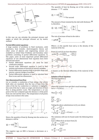
Find the transfer function of the system shown below?

Transfer function: It is the relation between the output
and the input of a dynamic system written in complex
form (s). For a dynamic system with an input u(t) and an
output y(t) ,the transfer function H(s) is the ratio between
the complex representation (s) of the output Y(s) and
input U(s).
Whenever they give any mechanical translation system,
mass desk pot, spring will be in mechanical system. When
we have to find out the transfer function of the system we
need to take the output transfer by input
is in terms of # and input in terms ‡$. If we consider
we get transfer function of the system as fallow
First mass X$, second mass X
Force due to the mass X$ is ‡X$ X$
QF
Q4
Taking Laplace Transform both side
0 X , P , ‚$ , ŠP , P$ , ‹
0 P , X , + ‚$ , + ‚ , Œ
P$ ,
`F ;F 8 •Ž ; 8 •F ; 8 •F •F ;
•Ž ;8 •F

b$ , X$ , + ‚$ , Œ$ Œ
`F ;F 8 •
b$ , P , ‘
Š `Ž ;F 8 •Ž ;8 •Ž8 •F ‹ Š`F ;F
•
•F ;
’Ž ;
‘
•Ž ; 8 •F
`Ž ;F 8 •Ž ;8 •Ž8 •F `F ;F 8 •Ž ; 8 •F
It is a transfer function of given mechanical
CONCLUSION
In this paper we conclude that mathematics is backbone in
study of technical subject of Mechanical Engineering.
Mathematics is applied in various field of mechanical
engineering like maths is use in fluid mechanics, straight
of material, machine design etc. In this way mathematical
concept and procedure are used to solve problem in above
mentioned field.
References
[1] Musadoto, Strength of Materials, 1st
pp 1-15.
[2] Mayur Jain, “Application of Mathematics in civil
Engineering”, International Journal of Innovations
in Engineering and Technology (IJIET), Volume 8
Issue 3 June 2017.
Transfer function: It is the relation between the output
and the input of a dynamic system written in complex
form (s). For a dynamic system with an input u(t) and an
output y(t) ,the transfer function H(s) is the ratio between
on (s) of the output Y(s) and
Whenever they give any mechanical translation system,
mass desk pot, spring will be in mechanical system. When
we have to find out the transfer function of the system we
transfer .Output
If we consider
•F ;
“Ž ”
we get transfer function of the system as fallow
Ž
4F
Force due to the spring Œ$ is
Force due to the desk pot ‚$ is
Force due to the spring Œ is
External force is equal to the sum of all internal forces.
‡$ M ‡X$ ‡Œ$ ‡‚$
‡$ M X$
QF
Ž
Q4F Œ$#$ ‚$
Taking Laplace transform both side, we get
b$ , X$ , P$ ,
P , Œ P$ , P ,
b$ , X$ , + ‚$ ,
Œ P , .
Force acting on mass X .
Force due to the mass X .,
Force due to the desk pot ‚$ is
Force due to the desk pot ‚
Force due to the spring Œ is
No external force acting on mass
0 ‡X ‡‚$ ‡‚ ‡Œ
0 X
QF
F
Q4F ‚$
Q
Q4
# #
‹ ‚ , P , Œ P , P$ ,
P$ , ‚$ , Œ
•Ž ; 8 •F ; 8 •F •F ;
•Ž ;8 •F
‚$ , Œ P ,
F 8 •Ž ; 8 •F ; 8 •F ‹•F ; C •Ž ; 8 •F
F
•Ž ; 8 •F
•
; 8 •F •F ; C •Ž ; 8 •F
F •
It is a transfer function of given mechanical system.
In this paper we conclude that mathematics is backbone in
study of technical subject of Mechanical Engineering.
Mathematics is applied in various field of mechanical
mechanics, straight
of material, machine design etc. In this way mathematical
concept and procedure are used to solve problem in above
st ed, IWRE, 2018,
athematics in civil
Engineering”, International Journal of Innovations
in Engineering and Technology (IJIET), Volume 8
[3] Ananda K. and Gangadharaiah Y. H.” Applications of
Laplace Transforms in Engineering and Economics”
(IJTSRD) Volume 3(1), ISSN: 2394
[4] Aye Aye Aung1, New Thazin Wai2” How Apply
Mathematics in Engineering Fields “(IJTSRD)
Volume 3 Issue 5, August 2019.
[5] Dr. B. B Singh, A coarse in Engineering mathematics,
1st ed, Vol III, Synergy knowledge ware, pp 4.1
4.76.
[6] B. S. Grewal, Higher Engineering Mathematics, 13
edition, Khanna publisher, pp 564
[7] P. N. Wartikar and J.N. Wartikar, A text book of
Applied Mathematics, Volume 3,1
Vidyathri Griha Prakashan, pp 463
[8] H. K Dass, Advanced Engineering
edition, S.Chand Publication, pp 720
‡Œ$ Œ$#$
is ‡‚$ ‚$
Q
Q4
#$ #
‡Œ Œ #$ # )
External force is equal to the sum of all internal forces.
‡Œ
Q
Q4
#$ # Œ #$ # )
Taking Laplace transform both side, we get
Œ$ P$ , ‚$ , P$ ,
,
Œ$ Œ P$ , ‚$ ,
‡X X
QF
F
Q4F
is ‡‚$ ‚$
Q
Q4
# #$
is ‡‚ ‚
Q F
Q4

‡Œ Œ # #$
No external force acting on mass X
#$ ‚
Q F
Q4
Œ # #$
Ananda K. and Gangadharaiah Y. H.” Applications of
Laplace Transforms in Engineering and Economics”
3(1), ISSN: 2394-9333
Aye Aye Aung1, New Thazin Wai2” How Apply
Mathematics in Engineering Fields “(IJTSRD)
Volume 3 Issue 5, August 2019.
A coarse in Engineering mathematics,
ed, Vol III, Synergy knowledge ware, pp 4.1 –
ewal, Higher Engineering Mathematics, 13th
Khanna publisher, pp 564 – 571.
N. Wartikar and J.N. Wartikar, A text book of
Applied Mathematics, Volume 3,1st ed, Pune
Vidyathri Griha Prakashan, pp 463-584.
K Dass, Advanced Engineering Mathematics, 19th
edition, S.Chand Publication, pp 720-723.

Application of Mathematics in Mechanical Engineering

More Related Content

What's hot

Similar to Application of Mathematics in Mechanical Engineering

More from ijtsrd

Recently uploaded

Application of Mathematics in Mechanical Engineering