Estimation of mean and its function using asymmetric loss function

International Journal of Soft Computing, Mathematics and Control (IJSCMC), Vol.2, No.1, February 2013
27
Estimation of mean and its function using
asymmetric loss function
BinodKumar Singh
University of Petroleum & Energy Studies, Dehradun, Uttrakhand, India.
singhbinod4@yahoo.co.in, bksingh_ism@yahoo.co.in
Abstract
In this paper suggested an improve estimator for mean using Linex loss function and shows that the
improved estimator dominates the Searls (1964) estimator underLinex loss function. The sufficient statistics
can be used to find the uniformly minimum risk unbiased estimators. In this paper an improve estimation
forµ2
is suggested (which uses coefficient of variation) under Linex loss function. The mathematical
expression of improve estimator of fourth power of mean is also obtained and an improve estimator for
common mean in negative exponential distribution is also proposed under Linex loss function.Pandey and
Malik (1994) considered the estimator yxwywxwT 3
2
2
2
11 ++=′ for common mean with the
restriction .1321 =++ www Here considered the above estimator for 1321 ≠++ www and studied its
property under Linex loss function. In this paper alsoconsidered the displaced exponential distribution
under Linex loss function and suggested an improve estimator.
Key Words
Linex loss Function, Mean square error and risk
1.Introduction
Let x1, x2, ........., xn be a random sample of size n from the normal population with mean µ and
variance
2
σ .We know that the sample mean
n
x
x i∑
= is sufficient and unbiased estimator for
population mean with minimum variance
n
2
σ
. The usual practice to compare the estimators based
on mean square error (MSE) for location parameter and may not yield a clear favorite for scale
parameter. One way to make the problem of finding a ‘best estimator tractable is to limit the class
of estimators. A popular way of restricting the class of estimators by consideringunbiased and
invariance estimators.
Searls (1964) has suggested the improved estimator '
2
nx
Y
n ϑ
=
+
in the class of estimators xcY ='
and show that

28
( ) ( )
12 2 2
'
1MSE Y MSE x
n n n
σ ϑ σ
−
 
= + < = 
 
. (1.1)
In negative exponential distribution (N.E.D.) with E(x)=θ, V(x) = θ2
andϑ=1. The improved
estimator is
1
1
+
=
n
xn
Y with
1
)(
2
1
+
=
n
YMSE
θ
which is smaller then
n
2
θ
,θ is the scale
parameter. In normal distribution having mean µ and variance σ2
, where σ2
behaves as scale
parameter and the maximum likelihood estimate is ( ) ( )
22
1
1
S x x MLE
n
= −∑ and
( )
22
1
1
1
s x x
n
= −
−
∑ (the unbiased estimator) are the estimators for σ2
.
Thus ( )
4
2 2
MSE S
n
σ
= and ( ) 1n
2
sMSE
4
2
−
σ
= .
Varian (1975) proposed the Linex (linear-exponential) lossfunction. The equation of Linex loss is
( ) ˆ, 1 , , 0,a
L a b e a aµ µ∆
 ∆ = − ∆ − ∆ = − ≠  (1.2)
Where a and b are shape and scale parameter respectively.
If 0a → , the Linex loss reduce to squared error.
The Linex loss function which rises exponentially on one side of zero and almost linearly on the
other side of zero. This loss function reduce to squared error loss for value of a near to zero.
Sadooghi(1990) considered theLinex loss for estimating the binomial parameter. Zellner (1986)
used this loss function for estimating the mean of a normal distribution. Basu and Ebrahim (1991)
considered this loss function in the context of reliability estimation in exponential distribution.
Pandey and Rai (1992) considered Bayesian estimation of mean and square of mean of normal
distribution using Linex loss function. The sufficient statistics can be used to find the uniformly
minimum risk unbiased (UMRU) estimator underLinex loss function (Bell, 1968)). If over-
estimation and under-estimation are present in practical situations (just as life testing, quality
control, engineering statistics), the Linex loss function can be applied (Pandey, 1997), (Pandey
&Srivastava, 2001), (Rojo, 1987), (Zellner, 1986), (Pandey and Rai ,1992).The MMSE criterion is
inadmissible under Linex loss function.
In section 2, suggested an improve estimator for mean using Linex loss function and shows that
the improved estimator dominates the Searls (1964) estimator underLinex loss function. The
sufficient statistics can be used to find the uniformly minimum risk unbiased estimator.
In section 3, an improve estimation forµ2
is suggested (which uses coefficient of variation) under
Linex loss function.
The mathematical expression of improve estimatorof fourth power of mean is also considered in
section 4.

29
In section 5, an improve estimator for common mean in negative exponential distribution is
proposed under Linex loss function.
In section 6,Pandey and Malik (1994) considered the yxwywxwT 3
2
2
2
11 ++=′ for
common mean with the restriction 1321 =++ www .Here considered the above estimator for
1321 ≠++ www . and studied its property
In section 7, considered the displaced exponential distribution under Linex loss function and
suggested an improve estimator.
2. Estimation of mean using Linex loss function
Zellner (1968) proposed the Linex loss function
( ) 0,),1(, ≠−=∆−∆−=∆
Λ
∆
acebaL a
µµ andif bc=a ,then this function will be equal to
)1( −∆−∆
aeb a
The Linex loss function reduce to squared error if 0a → .
Basu and Ebrahimi (1991) considered the invariant form of Linex loss for estimating µ .
The invariant form of Linex loss is
( ) .0,1),1(, ≠−=∆−∆−=∆
Λ
∗∗∆∗ ∗
acebaL a
µ
µ
( ) ( )[ ] ....1
3
1
2
,,
322
**








+





−+





−=∆=∆
µµ
xc
E
axc
E
a
aLEaR , where xc=
∧
µ
( )
2 3
*
2
2
, 1 1 ...
3
x a x
R a E E
a µ µ
      
∆ = − + − +      
         
. (2.1)
Let us consider an estimator xcY =1 in case of normal distribution with mean µ and variance 2
σ .
The invariant form of Linex loss is
( ) .11,
1
*
−





−−=∆






−
µ
µ xc
aeaL
xc
a
( ) ( )
1, 12*
222
−+−=∆ −−
aaceeaR can
ca ϑ
.
( ) ( ) ( ) 12
2
3
1)
12
3
3
2
2(
2
1
2
223
1
3
3
,
2
2 aaaa
aae
n
vcae
n
vac
aR
a
+−+−+−−−++−+=∗∆ (2.2)

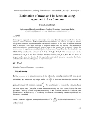
30
In negative exponential distribution, we have,
nxca
n
ac
eE
−






−=








1θ
(2.3)
And
( ) .1
1
, *
−+−






−
=∆ aac
n
ac
e
aR n
a
(2.4)
From equation (2.4), we get the minimum value of c as








−= +1
min 1 n
a
e
a
n
c (Pandey (1997). (2.5)
The proposed estimator is xe
a
n
Y n
a








−= +1
1 1 with ( )=∆*
,aRMin ( ) 







−+− +1
1 n
a
eana .
Thus minimum mean squared error is inadmissible under Linex loss function.
Differentiating equation (2.2) with respect to c and equating to zero, we get,
It will be minimum if
( )
















+
+−+





+−++−
=
)
3
1(
)
3
1)(
2
(411)1)(1(
2
2222
2
2
min
n
v
a
n
va
a
n
v
a
n
v
a
c (2.6)
For given values of ,n ϑ ≥1 and 0≤a≤0.6, the values of c can be obtained. Putting the cmin in
equation (2.2) we obtained the minimum risk. Figure 2.1 to 2.3, represent the relative efficiency of
the estimator Y1with respect to
'
'
Y for ϑ = 1.00(.25)1.50, and n = 5(5)20 and a = .4(.2).8.
The figure shows that if ν ≥1, the estimator perform better for smaller values of n and the values of
aupto 2.00.
Pandey and Rai(1992) considered the Bayes estimator for mean and square of population mean of
normal distribution under Linex loss function. Pandey (1997) obtained the result for scale

31
parameter in case of negative exponential distribution using invariant version of Linex loss
function as .1 1
1 xe
a
n
Y n
a








−= +
.
)1(6)1(21 321 −−−−
+
+
+
−
+
=
n
xan
n
xan
n
xn
Y
We know that
θ
xn2
follows a chi-square distribution with 2n degrees of freedom (Gamma (1, n)).
Bell(1968) defined a modified Bessel function as
( )
( ) ( )( )
2 2 2 3 3 3
2 4 8
2 1 ...
1! 2! 1 1! 1 2
n
na x a n x n a x
H na x
n n n n n n
= + + + +
+ + +
( )
...
1n2
xna4
xa21
22
+
+
++=
( )[ ] ....4
!2
212 22
2
θ
θθ a
n e
a
axnaHE =+++=
( )[ ] ( )[ ] θ=⇒θ= xan2HElog
a2
1
a2xna2HElog nn .
This MVRU estimator for θ is
( )
............
1
ˆ
2
+
+
−=
n
xa
xθ
This shows that sufficient statistics x can be used to find UMRU estimator in Linex loss function.
3. Estimation of square of mean usingLinex loss function
In normal distribution, we know that ( )
n
xV
2
σ
= which implies
n
1
x
ˆ
2
2
2
ϑ
+
=µ .
If we consider 2
22 xtY = , the minimum value of t2 is
2
2min 22 2
2
1
1
2
1 4
nt
n n n
ϑ
ϑ ϑ
ϑ
+
= ≤
   
+ + +   
  

32
Therefore the proposed estimator is












+
+
++
=
n
n
n
x
Y
2
2
2
2
2
1
2
4
11
ϑ
ϑ
ϑ
if ϑ is known.
If ϑ is unknown, the MVUE for
2
µ is
2
2 s
U x
n
= − .
For smaller value of n, U may be negative and Das (1975) suggested a biased estimator for 2
µ as
D=
12
2
2
1
s
x
ny
−
 
+ 
 
and studied its large sample properties. To obtain an estimator which has
same mean square error as D for large sample size n but has smaller bias in D, Pandey (1980)
suggested an estimator
The invariant form of Linex loss function for the estimator 2
44 xtY = is
.11),( 2
4
2
2
4
2
−





−−=∆ −∗
µ
µ txa
aeeaL
txa
a
(3.1)
.11),( 2
4
2
2
4
2
−





−−








=∆ −∗
µ
µ txa
aEeEeaR
txa
a
(3.2)
( ) .
123
1)1)(
123
2(
23
,
2 2
4
232
4
42
4
6
63
4
2
aa
t
n
vaa
ae
x
E
t
e
x
E
at
aR
a
aa
+−++−+−−





+





=∆ −−∗
µµ
Differentiating this equation w r to 4t and equating to zero, we have
.
2
)1)(
123
2()(
6
6
4
4232
4
4
2
4
4
4












+−+−++





−
=
µ
µµµ
x
aE
x
E
n
vaa
ae
x
E
x
E
t
a
m
2
2 2
2 2
1 1
x
P
s s
ny ny
=
 
+ + 
 

33
which indicate that 0≤ mt4 ≤1.
Pandey and Singh (1977) proposed the improved estimator 10, 5
2
55 ≤≤= cxcY in case of
negative exponential distribution. In case of N.E.D. with E (θ,θ) we have ( ) 22 1
θ
n
n
xE
+
= and
( ) ( )( )( ) .
123 4
3
4
θ
n
nnn
xE
+++
=
The invariant form of Linex loss function is
( ) .11, 2
2
5* 2
2
5
−





−−=∆ −
θ
θ
xc
aeeaR a
xac
which has
( ) .
3
1
)1
2
)(1(2
)1)(2)(3()1(
3
)1)(2)(3)(4)(5(
,
2 5
3
2
5
5
3
5
2
a
n
a
nc
n
nnnca
n
nnnnnac
aR
a
−+
−+
+
+++−
+
+++++
=∆∗
(3.3)
Differentiating this equation with respect to 5c and equating to zero, we get
0
)1
2
)(1(2
)1)(2)(3()1(2)1)(2)(3)(4)(5(
3
5
5
2
5
=
−+
+
+++−
+
+++++
n
a
n
n
nnnca
n
nnnnnac
.
Again differentiating equation (3.3) with respect to 5c we get,
)4)(5(
)1( 2
5
++
−
≥
nna
na
c and c5 must lies between 1
)4)(5(
)1(
5
2
≤≤
++
−
c
nna
na
Differentiatingequation (3.3) with respect to c5 and equating to zero, we have
.
)1)(2)(3)(4)(5(2
)1
2
()1)(2)(3)(4)(5(8
)1()2()3()1(4)1)(2)(3)(1(2
5
6
2
6
2222
3
min5
n
nnnnn
n
a
nnnnn
n
nnna
n
nnna
c
+++++
−+++++
−
+++−
+
+++−
=

34
4. Estimation of fourth power of mean under Linex loss function
Let us consider anestimator for the fourth power of mean as
4
66 xtY = . We have
( )
2 2 4 2 4
4 4 4
2 2
6 3
1 6 3E x
n n n n
µ σ σ ϑ ϑ
µ µ
 
= + + = + + 
 
and
8
2
2
42
6
4
66 1
36
1)()( µ





−






+++=
n
v
n
v
txVtYMSE .
The values of 6t for which )( 6YMSE will be minimum can be obtained.
In negative exponential distribution with
θ
xn
v
2
and1= follows the Chi- square with 2n defend
( ) ( )( )( ) 4
3
4 123
θ
n
nnn
xE
+++
= ,
( ) ( )( )( )( )( )( )( )



−
+++++++
=
8
4
n
n1n2n3n4n5n6n7n
xV
( ) ( ) ( ) 8
8
2222
n
n1n2n3n
θ



+++ .
( ) ( ) ( ).4
6
242
66 xtBiasxVtYMSE +=
The minimum value of t6 for which MSE (Y6) will be minimum is
( )( )( )( )
.
4567
4
min6
++++
=
nnnn
n
t (4.1)
The invariant form of Linex loss function in negative exponential distribution is
( ) .1, 4
4
6
* 4
4
6
−+−=∆ a
x
ateeaL
xat
a
θ
θ (4.2)
( ) ( )( )( ) a
et
n
nnnaaaa
aR
a
+




 +++






+−−





+−=∆ 63
22
*
2
123
...
3!1
2...
3.43
1,
2
( )( )( )( )( )( )( ) a
e
a
t
n
nnnnnnn
3
1234567 2
67
+
+++++++
( )( )( )( )( )( )( )( )( )( )( ) .
1234567891011 3
611
t
n
nnnnnnnnnnn +++++++++++
(4.3)

35
Differentiating this equation with respect to t6 and equating to zero, we get the value of t6 min.
If 0,a → we get the values according to equation (4.1).
5. Estimation of combine mean under Linex loss function
Let 1i n,........2,1i,x = and yj 2n....,2,1j = be the random samples of sizes n1 and n2from two
exponential distributions with parameters θ1 and θ2 respectively. The combineestimator for mean
is
( )1 2 1'
2 1 2
1
1
a
n n
Y e n x n y
a
−
+ +
 
= − + 
 
 
. (5.1)
With ( ) ( ) 1 2( 1
2 1 2 1 1
a
n n
Min R Y a n n e + +
 
= − + + − 
 
 
for pooled estimator under Linex loss function
when θ=θ=θ 21 .
For squared error 0a → and MMSE estimator is
1
ˆ
21
21
++
+
=
nn
ynxn
mθ which is inadmissible under
L (∆*
) (Rai (1996)).
If means of two populations are same but variances are unequal, the estimator for common mean is
( ).216
2
2
2
2
1
1
2
2
2
2
1
1
6
2
2
2
2
1
1
2
2
2
2
1
1
67 ylxlt
nn
ynxn
t
nn
ynxn
tY +=












+
+
≈






+
+
=
ϑϑ
ϑϑ
σσ
σσ
, (5.2)
where ( )2 1 2
1 1 1 2 1 1 22 2
1 2
/ / , 1 , &
n n
l n l lϑ ϑ ϑ
ϑ ϑ
 
= + = − 
 
are known.
The invariant form of Linex loss function is
( ) 6* 1 2 1 2
6, 1ata l x l y l x l y
L a e e a t a
µ µ
   + +
∆ = − + −  
   
(5.3)
( ) 1a
ylxl
tEa
ylat
eE.
xlat
eEe,aR 21
6
2616a*
−+





µ
+
−





µ





µ
=∆ (5.4)

36
In normal distribution, we have
6 2
6 1
12 2 2 2 2 2 2 2
6 1 6 1 1 6 2 6 2 22
1 2
,
2
at lat lat l x a t l at l y a t l
E e e E e e
n n
ϑ ϑ
µ µ
+   
= + =   
   
Therefore from equation (5.4) we have,
where
2
2
2
2
1
1
1
nn
1
p
ϑ
+
ϑ
= .
Differentiating with respect to t6 and equating to zero, we get
If a = o we have
2
2
2
1
2
12
2
21
2
12
2
21
6
nn
nn
t
ϑϑ+ϑ+ϑ
ϑ+ϑ
= (Pandey& Singh (1978)). (5.5)
In case of N.E.D. and if, 1,1 21 =ϑ=ϑ then
21
1
1
nn
n
l
+
= ,
21
2
2
nn
n
l
+
= and improved
estimator is
1 2
6
1 2 1
n x n y
Y
n n
+
=
+ +
.
The improved estimator under Linex loss can be obtained.
( ) ( ) 3
61
2
616
322
*
2
3
1..
3.43
2..
3.43
1,
2
teap
a
tpet
aa
a
aa
aR
a
aa






++++





+−+−−





+−=∆
( ) ( ) 0312..
3.43
2 2
6161
32
=++++





−+−− teapatpe
aa
a aa

37
6. Estimation of square of common mean in negative exponential
distribution
Suppose the estimator for square of common mean µ as
( )
2 2 2 2 2
1 2 1 2 1 2
7 2
1 2 1 2
2n x n y n x n y n n x y
Y
n n n n
 + + +
= = 
+ + 
.
Pandey and Malik (1994) proposed the estimator for µ2
is negative exponential distribution under
the squared error loss function as
yxwywxwT 3
2
2
2
11 ++=′ (6.1)
where w1, w2 and w3 are weights and
( ) ( ) ( ) ( ) 6nn5nn
n
w,
6nn5nn
n
w
21
2
21
2
2
2
21
2
21
2
1
1
++++
=
++++
=
( ) ( ) 6nn5nn
nn2
w
21
2
21
21
3
++++
=
The improved estimator is
( ) ( ) 6nn5nn
yxnn2ynxn
"T
21
2
21
21
22
2
22
1
1
++++
++
= with
MSE( ) ( )
( ) ( )
.
65
3222
"
21
2
21
21
1
++++
++
=
nnnn
nn
T (6.2)
The invariant form of Linex loss for the estimator { }yxwywxwtY 3
2
2
2
188 ++= is
( )
2 2 2 2
* 1 2 2 1 2 28, 182 2
w x w y w xy w x w y w xyta
L a e e at a
µ µ
+ + + +
∆ = − + −
      
   
      
. (6.3)

38
If x and y are independent negative exponential distributions, we have
( )
( ) ( )
( ) ( )
2 2 3
1 1 2 2 1 2*
822
1 2 1 2
1 1 22
, 1 .. 2 ..
3 4.3 3 4.3 5 6
n n n n nna a a a
R a a t
a n n n n
 + + + +   
 ∆ = − + − − + − +    + + + +    
( ) ( )[ ]
( )( )( ) ( )( )( )[ 3n2n1nn3n2n1nn
6nn5nn
e
222211112
21
2
21
a
+++++++
++++
+
( ) ( ) ( ){ } 2
1 2 1 2 1 2 1 1 2 2 86 1 ( 1) 4 1 1n n n n n n n n n n t+ + + + + + + 
( ) ( )
( )( )( ) ( ) ( ) ( )1 1 1 1 1 1 2 232
1 2 1 2
1
1 2 3 4 5 1
3 5 6
a
ae
n n n n n n n n
n n n n
+ + + + + + + +
 + + + +
 
( )( ) ( )( ) ( )( ) ( )( ) 2
2
2
12211212222 nn122n1n2n1nnn85n4n3n2n ++++++++++
( ) ( ) ( ) ( ) ( ) ( ) ( ) ( )
22 2
1 2 1 1 2 2 1 2 1 1 1 2 21 1 12 1 1 6 1 2 3 12 1n n n n n n n n n n n n n+ + + + + + + + + + +
( ) ( ) ( ) ( ) ( )( )( )( )
22 2
1 1 1 2 2 2 2 1 2 1 1 1 21 6 1 2 3 3 1 2 3 1n n n n n n n n n n n n n+ + + + + + + + + +
( )( )( )( )] .32113 222121 +++++ nnnnnn (6.4)
If a=0 (squared error), we have
( ) ( )
( ) ( )
+
++++
++++
−=



 ∆ 8
21
2
21
212211*
2
t
6nn5nn
nn21nn1nn
21,aR
a
2
( )( )( ) ( )( )( ) ( )
( ) ( ){ }
( ) ( )
1 1 1 1 2 2 2 2 1 2 1 2
1 2 1 1 2 2
822
1 2 1 2
1 2 3 1 2 3 6 1 ( 1)
4 1 1
5 6
n n n n n n n n n n n n
n n n n n n
t
n n n n
 + + + + + + + + + +
 
+ + +  
 + + + +
 

39
Differentiating equation (6.4) with respect to t8 and equating to zero we get,
( ) ( ) ( )( )
( )( )( ) ( )( )( ) ( )( )
( ) ( ){ }
2
1 2 1 2 1 2 1 2
8min
1 1 1 1 2 2 2 2 1 2 1 2
1 2 1 1 2 2
5 6 1
1 2 3 1 2 3 6 1 1
4 1 1
n n n n n n n n
t
n n n n n n n n nn n n
nn n n n n
 + + + + + + +
 =
 + + + + + + + + + +
 
+ + + +  
If n2=0, we get min8t = 1 and the improved estimator is
( )( )3n2n
xn
Y
11
22
1
2
++
=
The relative efficiency for different values of a, n1=5(5) 20 and n2=5(5)10 20
were calculated in Table 6.1.
The table 6.1, showsthat if a>1 the relative efficiency increases if n2 increases. Again for fixed n2
the relative efficiency increases for increasing n1 of scale and its function.
7.Estimation of displaced exponential distribution underLinex loss
function
Let x1, x2, ......,xn be a random sample of size n from a displaced exponential distribution having
p.d.f.
( ) ( ) 0,Ax,
Ax
e
1
,A,xf >θ>
θ
−
θ
=θ (7.1)
Here A is location and θ is scale parameters. The maximum likelihood estimators for θ and A are
( ))1(xx − and (1)x respectively.
We know that
( )( )
θ
− 1xxn2
follows a chi-square distribution with 2(n-1) degrees of freedom.
Thus ( )( ){ } ( )( ){ } ( )( )
2
1 1 12
1 1
,
1
n n n
E x x V x x x x
n n n
θ θ
− −   
− = − = ⇒ −   
−   
is unbiased
estimator for θ2
.

40
The invariant form of Linex function for the estimator ( )( )'
1 1 1
D l x x= − is
( )
( )( )( )
( )( )'
1 1 '
1 1*
, 1
l x x
a
a
l x x
L a e e a aθ
θ
−
−
 − 
∆ = − + − 
  
( )
( )( )'
1 1
* '
1
1
, 1
l x x
a
a n
R a e E e a l a
n
θ
−
−
 
 −  ∆ = − + −      
 
.We have
( )( ) ( )'
1 1 1'
1
1
nl x x
a al
E e
n
θ
− −−     = − 
    
and ( ) ( )
* '
11'
1
1
, 1
1
a
n
e n
R a a l a
nal
n
−
−
 − 
∆ = − + −  
   
− 
 
Differentiating with respect to
'
1l and putting equal to zero, we have
( )1 1'
11 ( 1)
( 1) 1 0
n
a al n
n ae a
n n n
− − −
−   −
− − − = 
 
Thus,
' '
1 1
1 1 1
n a
a n
al al
e e
n n
−
−  
− = ⇒ = − 
 
or,
'
1 1
a
n
n
l e
a
 
= − 
 
.
The improved estimator is
( )( ) ( )( )
2
1 1 12
1 1 1
2
a
n
n n a a
D e x x x x
a a n n
    
= − − = − − + − −    
    
( ){ } ( )( ) ( ){ }
2 2
1 1 12
1 1 .... ....
2 2
n a a a
x x x x x x
a n n n
 
= − + − + − = − − − + 
 
Thus ( )( )1
x x− is improved estimator for θ if 0→a (squared error). We know that
( ){ }2
1xx
1n
n
−
−
is unbiased estimator for θ2
.

41
8. References
[1] Basu, A.P. and Ebrahimi, N. (1991) “Bayesian approach to life testing and
reliabilityestimation using asymmetric loss function.”Jour. Stat. Plann. Infer, 29, 21-31.
[2] Bell, W.W. (1968) “Special Function for Scientists and Engineers”, London: Van Nostrand.
[3] Das, B.(1975) Estimation of µ2
in normal population,Cal.Stat.Assn.Bull.,24,135-140.
[4] Pandey,B.N.(1980) “On estimation of variance in normal
distribution”.Jour.Ind.Soc.Agri.Stat.33,1-5.
[5] Pandey, B.N. (1997) “Testimator of the scale parameter of the exponential distribution using
[6] Linexloss function.” Comm. Stat.Theo.Meth.,26, 2191-2200.
[7] Pandey, B.N.and Malik, H.J. (1994) “Some improved estimators for common variance of
two
[8] populations.” Comm. Stat. Theo. Meth., 23(10), 3019-3035.
[9] Pandey, B.N.andRai, Omkar (1992) “Bayesian estimation of mean and squares of mean of
[10] normal population distribution using Linex loss function.” Comm. Stat.Theo.Meth.21 (12),
[11] 3369-3391.
[12] Pandey, B.N.and Singh, K.N. (1978) “A pre-test shrinkage estimator of mean of a
normalpopulation.”Jour.Ind.Soc.Agri.Stat.30, 91-98.
[13] Pandey, B.N.and Singh, J. (1977a) “Estimation of variance of normal population
usingapriori information.”Jour.Ind. Sta.Assoc.15, 141-150.
[14] Pandey, B.N.and Singh, J. (1977b) “A note on the estimation of variance in
exponentialdensity.”Sankhya 39, 294-298.
[15] Pandey, B.N.andSrivastava A.K. (2001) “Estimation of variance using asymmetric
lossfunction.”IAPQR.26 (2), 109-123.
[16] Rai,O.(1996) “A some-times pool estimation of mean life under Linex
lossfunction.”Comm.Sta.Theo.Meth.25, 2057-2067.
[17] Rojo, J. (1987) “On the admissibility of c x +d with respect to Linex loss function.”Comm.
[18] Stat.Theo.Meth.16, 3745-3748.
[19] Sadooghi-Alvandi, S.M. (1990) “Estimation of the parameter of a Poisson distribution using
[20] aLinex loss function.”Aust.Jour.Stat.32, 393-398.
[21] Searls, D.T. (1964) “The utilization of a known coefficient of variation in the
estimationprocedure.”Jour.Amer.Stat.Assoc.59, 1225-1226.
[22] Varian, H.R. (1975) “A Bayesian approach to real estate assessment.” In studies in Bayesian
[23] econometrics and statistics in honor of L. J. Savage, Eds S.E. Feinberge and A,
Zellner,Amsterdem North Holland, 195-208.
[24] Zellner, A. (1986) “Bayesian estimation and prediction using asymmetric loss
function.”Jour.Amer.Stat.Assoc.81, 446-451.

42
Appendices
a
n
5 10 15 20
.4 16.57 17.74 18.97 20.39
.6 8.6 9.65 11.43 13.57
.8 5.54 6.76 8.54 11.54
Table –2.1Relative efficiency of the estimator Y1 with respect to
'
Y for ϑ = 1.00
n
a
5 10 15 20
.4 10.31 10.82 11.29 11.78
.6 5.2 5.72 6.24 6.84
.8 3.3 3.74 4.25 4.8
Table –2.2Relative efficiency of the estimator Y1 with respect to
'
Y for ϑ = 1.25
n
a
5 10 15 20
.4 7.03 7.31 7.54 7.77
.6 3.2 3.76 3.99 4.25
.8 2.19 2.41 2.62 2.87
Table –2.3 Relative efficiency of the estimator Y1 with respect to
'
Y for ϑ = 1.50

43
Figure 2.1 Relative efficiency of the estimator Y1 with respect to
'
Y for ϑ = 1.00
Figure 2.2Relative efficiency of the estimator Y1 with respect to
'
Y for ϑ = 1.25
Figure 2.3Relative efficiency of the estimator Y1 with respect to
'
Y for ϑ =1.50
0
5
10
15
20
25
0.4 0.6 0.8
a
R.E.
n=5
n=10
n=15
n=20
0
2
4
6
8
10
12
14
0.4 0.6 0.8
a
R.E.
n=5
n=10
n=15
n=20
0
1
2
3
4
5
6
7
8
9
0.4 0.6 0.8
a
R.E.
n=5
n=10
n=15
n=20

44
n1
n2
5 10 15 20
5
(1) 1.431 1.638 1.631 1.585
(2) 1.509 1.744 1.751 1.715
(3) 1.603 1.877 1.904 1.884
(4)
(5)
1.686
1.717
1.990
2.016
2.032
2.051
2.026
2.037
10
(1) 1.638 2.418 2.729 2.789
(2) 1.744 2.629 3.008 3.108
(3) 1.877 2.903 3.381 3.544
(4)
(5)
1.990
2.016
3.133
3.146
3.698
3.691
3.918
3.890
15
(1) 1.631 2.729 3.478 3.855
(2) 1.751 3.008 3.916 4.410
(3) 1.904 3.381 4.528 5.216
(4)
(5)
2.032
2.051
3.698
3.691
5.061
5.001
5.936
5.818
20
(1) 1.585 2.789 3.855 4.581
(2) 1.715 3.108 4.410 5.356
(3) 1.884 3.544 5.216 6.542
(4)
(5)
2.026
2.037
3.918
3.890
5.936
5.818
7.648
7.404
(1) a =.2, (2) a= .4, (3) a = .6, (4) a=.8,(5) a=1.

Estimation of mean and its function using asymmetric loss function

Recommended

Recommended

More Related Content

What's hot

What's hot (17)

Similar to Estimation of mean and its function using asymmetric loss function

Similar to Estimation of mean and its function using asymmetric loss function (20)

Recently uploaded

Recently uploaded (20)

Estimation of mean and its function using asymmetric loss function