SlideShare a Scribd company logo
1 of 127
16 USING LINEAR REGRESSION PREDICTING THE
FUTURE
16: MEDIA LIBRARY
Premium Videos
Core Concepts in Stats Video
· Linear Regression
Lightboard Lecture Video
· Multiple Regression
Time to Practice Video
· Chapter 16: Problem 2
Difficulty Scale
(as hard as they get!)
WHAT YOU WILL LEARN IN THIS CHAPTER
· Understanding how prediction works and how it can be used in
the social and behavioral sciences
· Understanding how and why linear regression works when
predicting one variable on the basis of another
· Judging the accuracy of predictions
· Understanding how multiple regression works and why it is
useful
INTRODUCTION TO LINEAR REGRESSION
You’ve seen it all over the news—concern about obesity and
how it affects work and daily life. A set of researchers in
Sweden was interested in looking at how well mobility
disability and/or obesity predicted job strain and whether social
support at work can modify this association. The study included
more than 35,000 participants, and differences in job strain
mean scores were estimated using linear regression, the exact
focus of what we are discussing in this chapter. The results
found that level of mobile disability did predict job strain and
that social support at work significantly modified the
association among job strain, mobile disability, and obesity.
Want to know more? Go to the library or go online …
Norrback, M., De Munter, J., Tynelius, P., Ahlstrom, G., &
Rasmussen, F. (2016). The association of mobility disability,
weight status and job strain: A cross-sectional
study. Scandinavian Journal of Public Health, 44, 311–319.
WHAT IS PREDICTION ALL ABOUT?
Here’s the scoop. Not only can you compute the degree to which
two variables are related to one another (by computing a
correlation coefficient as we did in Chapter 5), but you can also
use these correlations to predict the value of one variable based
on the value of another. This is a very special case of how
correlations can be used, and it is a very powerful tool for
social and behavioral sciences researchers.
The basic idea is to use a set of previously collected data (such
as data on variables X and Y), calculate how correlated these
variables are with one another, and then use that correlation and
the knowledge of X to predict Y. Sound difficult? It’s not
really, especially once you see it illustrated.
For example, a researcher collects data on total high school
grade point average (GPA) and first-year college GPA for 400
students in their freshman year at the state university. He
computes the correlation between the two variables. Then, he
uses the techniques you’ll learn about later in this chapter to
take a new set of high school GPAs and (knowing the
relationship between high school GPA and first-year college
GPA from the previous set of students) predict what first-year
GPA should be for a new student who is just starting out. Pretty
nifty, huh?
Here’s another example. A group of kindergarten teachers is
interested in finding out how well extra help after for their
students aids them in first grade. That is, does the amount of
extra help in kindergarten predict success in first grade? Once
again, these teachers know the correlation between the amount
of extra help and first-grade performance from prior years; they
can apply it to a new set of students and predict first-grade
performance based on the amount of kindergarten help.
How does regression work? Data are collected on past events
(such as the existing relationship between two variables) and
then applied to a future event given knowledge of only one
variable. It’s easier than you think.
The higher the absolute value of the correlation coefficient,
regardless of whether it is direct or indirect (positive or
negative), the more accurate the prediction is of one variable
from the other based on that correlation. That’s because the
more two variables share in common, the more you know about
the second variable based on your knowledge of the first
variable. And you may already surmise that when the
correlation is perfect (+1.0 or −1.0), then the prediction is
perfect as well. If rxy = −1.0 or +1.0 and if you know the value
of X, then you also know the exact value of Y. Likewise,
if rxy = −1.0 or +1.0 and you know the value of Y, then you
also know the exact value of X. Either way works just fine.
What we’ll do in this chapter is go through the process of using
linear regression to predict a Y score from an X score. We’ll
begin by discussing the general logic that underlies prediction,
then review some simple line-drawing skills and, finally,
discuss the prediction process using specific examples.
Why the prediction of Y from X and not the other way around?
Convention. Seems like a good idea to have a consistent way to
identify variables, so the Y variable becomes the dependent
variable or the one being predicted and the X variable becomes
the independent variable and is the variable used to predict the
value of Y. And when predicted, the Y value is represented
as Y′ (read as Y prime)—the predicted value of Y. (To sound
like an expert, you might call the independent variable
a predictor and the dependent variable the criterion. Purists save
the terms independent and dependent to describe cause-and-
effect relationships, which we cannot assume when talking
about correlations.)THE LOGIC OF PREDICTION
Before we begin with the actual calculations and show you how
correlations are used for prediction, let’s understand the
argument for why and how prediction works. We will continue
with the example of predicting college GPA from high school
GPA.
Prediction is the computation of future outcomes based on a
knowledge of present ones. When we want to predict one
variable from another, we need to first compute the correlation
between the two variables. Table 16.1 shows the data we will be
using in this example. Figure 16.1 shows the scatterplot
(see Chapter 5) of the two variables that are being computed.
Table 16.1 ⬢ Total High School GPA and First-Year College
GPA
High School GPA
First-Year College GPA
3.50
3.30
2.50
2.20
4.00
3.50
3.80
2.70
2.80
3.50
1.90
2.00
3.20
3.10
3.70
3.40
2.70
1.90
3.30
3.70
Figure 16.1 ⬢ Scatterplot of high school GPA and college GPA
To predict college GPA from high school GPA, we have to
create a regression equation and use that to plot what is called
a regression line. A regression line reflects our best guess as to
what score on the Y variable (college GPA) would be predicted
by a score on the X variable (high school GPA). For all the data
you see in Table 16.1, the regression line is drawn so that it
minimizes the distance between itself and each of the points on
the predicted (Y′) variable. You’ll learn shortly how to draw
that line, shown in Figure 16.2.
What does the regression line you see in Figure 16.2 represent?
First, it’s the regression of the Y variable on the X variable. In
other words, Y (college GPA) is being predicted from X (high
school GPA). This regression line is also called the line of best
fit. The line fits these data because it minimizes the distance
between each individual point and the regression line. Those
distances are errors because it means the prediction was wrong;
it was some distance from the right answer. The line is drawn to
minimize those errors. For example, if you take all these points
and try to find the line that best fits them all at once, the line
you see in Figure 16.2 is the one you would use.
Second, it’s the line that allows us our best guess (at estimating
what college GPA would be, given each high school GPA). For
example, if high school GPA is 3.0, then college GPA should be
around (remember, this is only an eyeball prediction) 2.8. Take
a look at Figure 16.3 to see how we did this. We located the
predictor value (3.0) on the x-axis, drew a perpendicular line
from the x-axis to the regression line, then drew a horizontal
line to the y-axis, and finally estimated what the predicted value
of Y would be.
Figure 16.3 ⬢ Estimating college GPA given high school GPA
Third, the distance between each individual data point and the
regression line is the error in prediction—a direct reflection of
the correlation between the two variables. For example, if you
look at data point (3.3, 3.7), marked in Figure 16.4, you can see
that this (X, Y) data point is above the regression line. The
distance between that point and the line is the error in
prediction, as marked in Figure 16.4, because if the prediction
were perfect, then all the predicted points would fall where?
Right on the regression or prediction line.
Figure 16.4 ⬢ Prediction is rarely perfect: estimating the error
in prediction
Fourth, if the correlation were perfect (and the x-axis meets
the y-axis at Y ’s mean), all the data points would align
themselves along a 45° angle, and the regression line would
pass through each point (just as we said earlier in the third
point).
Given the regression line, we can use it to precisely predict any
future score. That’s what we’ll do right now—create the line
and then do some prediction work.CORE CONCEPTS IN
STATS VIDEOLinear RegressionDRAWING THE WORLD’S
BEST LINE (FOR YOUR DATA)
The simplest way to think of prediction is that you are
determining the score on one variable (which we’ll call Y—
the criterion or dependent variable) based on the value of
another score (which we’ll call X—the predictor or independent
variable).
The way that we find out how well X can predict Y is through
the creation of the regression line we mentioned earlier in this
chapter. This line is created from data that have already been
collected. The equations are then used to predict scores using a
new value for X, the predictor variable.
Formula 16.1 shows the general formula for the regression line,
which may look familiar because you may have used something
very similar in a high school or college math course. In
geometry, it’s the formula for any straight line:
(16.1)
Y'=bX+a,Y′=bX+a,
where
· Y ′ is the predicted score of Y based on a known value of X;
· b is the slope, or direction, of the line;
· X is the score being used as the predictor; and
· a is the point at which the line crosses the y-axis.
Let’s use the same data shown earlier in Table 16.1, along with
a few more calculations that we will need thrown in.
X
Y
X2
Y2
XY
3.5
3.3
12.25
10.89
11.55
2.5
2.2
6.25
4.84
5.50
4.0
3.5
16.00
12.25
14.00
3.8
2.7
14.44
7.29
10.26
2.8
3.5
7.84
12.25
9.80
1.9
2.0
3.61
4.00
3.80
3.2
3.1
10.24
9.61
9.92
3.7
3.4
13.69
11.56
12.58
2.7
1.9
7.29
3.61
5.13
3.3
3.7
10.89
13.69
12.21
Total
31.4
29.3
102.50
89.99
94.75
From this table, we see that
· ∑ X, or the sum of all the X values, is 31.4.
· ∑Y, or the sum of all the Y values, is 29.3.
· ∑ X 2, or the sum of each X value squared, is 102.5.
· ∑ Y 2, or the sum of each Y value squared, is 89.99.
· ∑ XY, or the sum of the products of X and Y, is 94.75.
Formula 16.2 is used to compute the slope of the regression line
(b in the equation for a straight line):
(16.2)
b=ΣXY−(ΣXΣY/n)ΣX2−[(ΣX)2/n].b=ΣXY−(ΣXΣY/n)ΣX2−[(ΣX)
2/n].
In Formula 16.3, you can see the computed value for b, the
slope of the line:
(16.3)
b=94.75−[(31.4×29.3)/10]102.5−[(31.4)2/10],b=2.7493.904=0.7
04.b=94.75−[(31.4×29.3)/10]102.5−[(31.4)2/10],b=2.7493.904=
0.704.
Formula 16.4 is used to compute the point at which the line
crosses the y-axis (a in the equation for a straight line):
(16.4)
a=ΣY−bΣXn.a=ΣY−bΣXn.
In Formula 16.5, you can see the computed value for a, the
intercept of the line:
(16.5)
a=29.3−(0.704×31.4)10,a=7.1910=0.719.a=29.3−(0.704×31.4)10
,a=7.1910=0.719.
Now, if we go back and substitute b and a into the equation for
a straight line (Y = bX + a), we come up with the final
regression line:
Y'=0.704X+0.719.Y′=0.704X+0.719.
Why the Y ′ and not just a plain Y ? Remember, we are
using X to predict Y, so we use Y ′ to mean the predicted and
not the actual value of Y.
So, now that we have this equation, what can we do with it?
Predict Y, of course.
For example, let’s say that high school GPA equals 2.8 (or X =
2.8). If we substitute the value of 2.8 into the equation, we get
the following formula:
Y'=0.704(2.8)+0.719=2.69.Y′=0.704(2.8)+0.719=2.69.
So, 2.69 is the predicted value of Y (or Y ′) given X is equal to
2.8. Now, for any X score, we can easily and quickly compute a
predicted Y score.
You can use this formula and the known values to compute
predicted values. That’s most of what we just talked about. But
you can also plot a regression line to show how well the scores
(what you are trying to predict) actually fit the data from which
you are predicting. Take another look at Figure 16.2, the plot of
the high school–college GPA data. It includes a regression line,
which is also called a trend line. How did we get this line?
Easy. We used the same charting skills you learned in Chapter
5 to create a scatterplot; then we selected Add Fit Line in the
SPSS Chart Editor. Poof! Done!
You can see that the trend is positive (in that the line has a
positive slope) and that the correlation is .6835—very positive.
And you can see that the data points do not align directly on the
line, but they are pretty close, which indicates that there is a
relatively small amount of error.
Not all lines that fit best between a bunch of data points are
straight. Rather, they could be curvilinear, just as you can have
a curvilinear relationship between your variables, as we
discussed in Chapter 5. For example, the relationship between
anxiety and performance is such that when people are not at all
anxious or very anxious, they don’t perform very well. But if
they’re moderately anxious, then performance can be enhanced.
The relationship between these two variables is curvilinear, and
the prediction of Y from X takes that into account. Dealing with
curvilinear relationships is beyond the scope of this book, but
fortunately, most relationships you’ll see in the social sciences
are essentially linear.
HOW GOOD IS YOUR PREDICTION?
How can we measure how good a job we have done predicting
one outcome from another? We know that the higher the
absolute magnitude of the correlation between two variables,
the better the prediction. In theory, that’s great. But being
practical, we can also look at the difference between the
predicted value (Y ′) and the actual value (Y) when we first
compute the formula of the regression line.
For example, if the formula for the regression line is Y ′ =
0.704X + 0.719, the predicted Y (or Y ′) for an X value of 2.8 is
0.704(2.8) + 0.719, or 2.69. We know that the actual Y value
that corresponds to an X value is 3.5 (from the data set shown
in Table 16.1). The difference between 3.5 and 2.69 is 0.81, and
that’s the size of the error in prediction.
Another measure of error that you could use is the coefficient of
determination (see Chapter 5), which is the percentage of error
that is reduced in the relationship between variables. For
example, if the correlation between two variables is .4 and the
coefficient of determination is 16% or .42, the reduction in
error is 16% since initially we suspect the relationship between
the two variables starts at 0 or 100% error (no predictive value
at all).
If we take all of these differences, we can compute the average
amount that each data point differs from the predicted data
point, or the standard error of estimate. This is a kind of
standard deviation that reflects average error along the line of
regression. The value tells us how much imprecision there is in
our estimate. As you might expect, the higher the correlation
between the two values (and the better the prediction), the lower
this standard error of estimate will be. In fact, if the correlation
between the two variables is perfect (either +1 or −1), then the
standard error of estimate is zero. Why? Because if prediction is
perfect, all of the actual data points fall on the regression line,
and there’s no error in estimating Y from X.
The predicted Y ′, or dependent variable, need not always be a
continuous one, such as height, test score, or problem-solving
skills. It can be a categorical variable, such as admit/don’t
admit, Level A/Level B, or Social Class 1/Social Class 2. The
score that’s used in the prediction is “dummy coded” to be a 0
or a 1 (or any two values) and then used in the same equation.
Yes, you are right that the level of measurement for this sort of
correlational stuff is supposed to be at the interval level, but a
variable with just two values works mathematically as if it has
equal-sized intervals because there is only one interval.
USING SPSS TO COMPUTE THE REGRESSION LINE
Let’s use SPSS to compute the regression line that predicts Y′
from X. The data set we are using is Chapter 16 Data Set 1. We
will be using the number of hours of training to predict how
severe injuries will be if someone is injured playing football.
There are two variables in this data set:
Variable
Definition
Training (X)
Number of hours per week of strength training
Injuries (Y)
Severity of injuries on a scale from 1 to 10
Here are the steps to compute the regression line that we
discussed in this chapter. Follow along and do it yourself.
1. Open the file named Chapter 16 Data Set 1.
2. Click Analyze → Regression → Linear. You’ll see the Linear
Regression dialog box shown in Figure 16.5.
3. Click on the variable named Injuries and then move it to the
Dependent: variable box. It’s the dependent variable because its
value depends on the value of number of hours of training. In
other words, it’s the variable being predicted.
4. Click on the variable named Training and then move it to the
Independent(s): variable box.
5. Click OK, and you will see the partial results of the analysis,
as shown in Figure 16.6.
We’ll get to the interpretation of this output in a moment. First,
let’s have SPSS overlay a regression line on the scatterplot for
these data like the one you saw earlier in Figure 16.2.
6. Click Graphs → Legacy Dialogs → Scatter/Dot.
7. Click Simple Scatter and then click Define. You’ll see the
simple Scatterplot dialog box.
8. Click Injuries and move it to the variable label to the Y Axis:
box. Remember, the predicted variable is represented by the y-
axis.
9. Click Training and move it to the variable label to the X
Axis: box.
10. Click OK, and you will see the scatterplot as shown
in Figure 16.7.
Now let’s draw the regression line.
11. If you are not in the chart editor, double-click on the chart
to select it for editing.
12. Click on the Add Fit Line at Total button (on the second
row of buttons, about fifth from the left) that looks a little like
this: .
13. Close the Properties box that opened when you selected the
Add Fit Line at Total button and then close the chart editor
window. The completed scatterplot, with the regression line, is
shown in Figure 16.8 along with the multiple regression
value R2, which equals 0.21. As you will read more about
shortly, the multiple regression correlation coefficient is the
regression of all the X values on the predicated value.
When you have the Properties dialog box open for drawing the
regression line, notice that there is a set of Confidence Intervals
options. When clicked, these show you a boundary within which
there is a specific probability as to how good the prediction is.
For example, if you click Mean and specify 95%, the graph will
show you the boundaries surrounding the regression line, within
which there is a 95% chance of the predicted scores occurring.
This idea of wanting to be within a certain range of error 95%
of the time is the same as wanting a .05 significance level for
statistical analyses.
Figure 16.5 ⬢ Linear Regression dialog box
Understanding the SPSS Output
The SPSS output tells us several things:
1. The formula for the regression line is taken from the first set
of output shown in Figure 16.6 as Y ′ = –0.125X + 6.847. This
equation can be used to predict level of injury given any number
of hours spent in strength training.
2. As you can see in Figure 16.8, the regression line has a
negative slope, reflecting a negative correlation (of –.458,
which is what Beta is in Figure 16.6) between hours of training
and severity of injuries. So it appears, given the data, that the
more one trains, the fewer severe injuries occur.
3. You can also see that the prediction is significant—in other
words, predicting Y from X is based on a significant
relationship between the two variables such that the test of
significance for both the constant (Training) and the predicted
variable (Injuries) is significantly different from zero (which it
would be if there was no predictive value for X predicting Y).
So just how good is the prediction? Well, the SPSS output
(which we did not show you) also indicates that the standard
error of estimate for Injuries (the predicted variable) is 2.182;
double that (4.36) and you’ll see that there is a 95% chance
(remember 1.96 or about 2 standard deviations away from the
mean creates a 95% confidence interval) the prediction will fall
between the mean of all injuries (which is 4.33) and ±4.46. So,
based on the correlation coefficient, the prediction is okay but
not great.
THE MORE PREDICTORS THE BETTER? MAYBE
All of the examples that we have used so far in the chapter have
been for one criterion or outcome measure and one predictor
variable. There is also the case of regression where more than
one predictor or independent variable is used to predict a
particular outcome. If one variable can predict an outcome with
some degree of accuracy, then why couldn’t two do a better job?
Maybe so, but there’s a big caveat—read on.
For example, if high school GPA is a pretty good indicator of
college GPA, then how about high school GPA plus number of
hours of extracurricular activities? So, instead of
Y'=bX+a,Y′=bX+a,
the model for the regression equation becomes
Y'=bX1+bX2+a,Y′=bX1+bX2+a,
where
· X1 is the value of the first independent variable,
· X2 is the value of the second independent variable,
· b is the regression weight for that particular variable, and
· a is the intercept of the regression line, or where the
regression line crosses the y-axis.
As you may have guessed, this model is called multiple
regression (multiple predictors, right?). So, in theory anyway,
you are predicting an outcome from two independent variables
rather than one. But you want to add additional predictor
variables only under certain conditions. Read on.
LIGHTBOARD LECTURE VIDEO
Multiple Regression
Any variable you add has to make a unique contribution to
understanding the dependent variable. Otherwise, why use it?
What do we mean by unique? The additional variable needs to
explain differences in the predicted variable that the first
predictor does not. That is, the two variables in combination
should predict Y better than any one of the variables would do
alone.
In our example, level of participation in extracurricular
activities could make a unique contribution. But should we add
a variable such as the number of hours each student studied in
high school as a third independent variable or predictor?
Because number of hours of study is probably highly related to
high school GPA (another of our predictor variables,
remember?), study time probably would not add very much to
the overall prediction of college GPA. We might be better off
looking for another variable (such as ratings on letters of
recommendation) rather than collecting the data on study time.
Take a look at Figure 16.9, which is the result of a multiple
regression analysis that adds the number of extracurricular
activity hours to the data you saw in Table 16.1. You can see
how both high school GPA and number of hours of
extracurricular activity are significant contributors to first-year
college GPA. This is a powerful way of examining what and
how more than one independent variable contribute to
prediction of another variable.
Figure 16.9 ⬢ A multiple regression analysis
The Big Rule(s) When It Comes to Using Multiple Predictor
Variables
If you are using more than one predictor variable, try to keep
the following two important guidelines in mind:
1. When selecting a variable to predict an outcome, select a
predictor variable (X) that is related to the criterion variable
(Y). That way, the two share something in common (remember,
they should be correlated).
2. When selecting more than one predictor variable (such
as X1 and X2), try to select variables that are independent or
uncorrelated with one another but are both related to the
outcome or predicted (Y) variable.
In effect, you want only independent or predictor variables that
are related to the dependent variable and are unrelated to each
other. That way, each one makes as distinct a contribution as
possible to predicting the dependent or predicted variable.
There are whole books on multiple regression, and much of
what one needs to learn about this powerful procedure is beyond
the scope of this book. Chapter 18 talks more about multiple
regression.
How many predictor variables are too many? Well, if one
variable predicts some outcome, and two are even more
accurate, then why not three, four, or
five predictor variables? In practical terms, every time you add
a variable, an expense is incurred. Someone has to go collect
the data, it takes time (which is $$$ when it comes to research
budgets), and so on. From a theoretical sense, there is a fixed
limit on how many variables can contribute to an understanding
of what we are trying to predict. Remember that it is best when
the predictor or independent variables are independent or
unrelated to each other. The problem is that once you get to
three or four variables, fewer things can remain unrelated.
Better to be accurate and conservative than to include too many
variables and waste money and the power of prediction.
Real-World Stats
How children feel about what they do is often very closely
related to how well they do what they do. The aim of this study
was to analyze the consequences of emotion during a writing
exercise. In the model this research follows, motivation and
affect (the experience of emotion) play an important role during
the writing process. Fourth and fifth graders were instructed to
write autobiographical narratives with no emotional content,
positive emotional content, and negative emotional content. The
results showed no effect regarding these instructions on the
proportion of spelling errors, but the results did reveal an effect
on the length of narrative the children wrote. A simple
regression analysis (just like the ones we did and discussed in
this chapter) showed a correlation and some predictive value
between working memory capacity and the number of spelling
errors in the neutral condition only. Since the model on which
the researchers based much of their preliminary thought about
this topic states that emotions can increase the cognitive load or
the amount of “work” necessary in writing, that becomes the
focus of the discussion in this research article.
Want to know more? Go online or to the library and find …
Fartoukh, M., Chanquoy, L., & Piolat, A. (2012). Effects of
emotion on writing processes in children. Written
Communication, 29, 391–411.
Summary
Prediction is a useful application of simple correlation, and it is
a very powerful tool for examining complex relationships. This
chapter might have been a little more difficult than others, but
you’ll be well served by what you have learned, especially if
you can apply it to the research reports and journal articles that
you have to read. We are now at the end of lots of chapters on
inference, and we’re about to move on in the next part of this
book to using statistics when the sample size is very small or
when the assumption that the scores are distributed in a normal
way is violated.
Time to Practice
1. How does linear regression differ from analysis of variance?
2. Chapter 16 Data Set 2 contains the data for a group of
participants who took a timed test. The data are the average
amount of time the participants took on each item (Time) and
the number of guesses it took to get each item correct (Correct).
a. What is the regression equation for predicting response
time from number correct?
b. What is the predicted response time if the number correct is
8?
c. What is the difference between the predicted and the actual
number correct for each of the predicted response times?
Time to Practice Video
Chapter 16: Problem 2
Chapter 16, Problem 2 will show you how to compute a linear
regression, so you can answer the question about the
regression equation and make some predictions. Doing a
regression is pretty straightforward. First, we want to go to our
SPSS Data Set, which is Chapter 16, Data Set 2. Once we're
here, we want to go to Analyze, then Regression, then Linear,
since we're using just two variables. When we click on Linear,
you want to think about where you place your dependent and
independent variables. The dependent is the outcome, or that
thing that is dependent on something else. In this case, the
number of correct answers is dependent on the amount of time
we think they spent on it. So, correct answers is the dependent
and time is the independent. Click OK, and our output pops
up. The key thing we're going to look at for making the
prediction is under Coefficients. And, for doing this, we're
going to look at the Unstandardized Beta Weights. Here you
see 7.414 and negative This is the two bits of information. So
let's refresh ourselves with what the data set looks like in
terms of creating a regression equation. This is the regression
equation. And so, what we have already, we figured out the
beta and then we figured out the point at which it crosses the
y-axis. When we put that information here, here is our
regression equation, y equals negative So, that's the equation
for Part A. Part B asks us to make a prediction. What is the
predicted time if the number of correct answers is 8? In this
situation, we take our regression equation, but now we add the
x, in this case 8, the number of correct answers, we do the
computation, and we come up with 6.262, which is the
predicted time. Part C asks you to determine the difference
between the predicted and actual time for each of them. And
then all you want to do there is, when you look at your data
set, is take the predicted and compute that, but instead of
putting in 8, put in each of these numbers, and come up and
compute the difference. And that's how we answer Chapter
16, Problem 2. Good luck.
1. Betsy is interested in predicting how many 75-year-olds will
develop Alzheimer’s disease and is using as predictors level of
education and general physical health graded on a scale from 1
to 10. But she is interested in using other predictor variables as
well. Answer the following questions:
a. What criteria should she use in the selection of other
predictors? Why?
b. Name two other predictors that you think might be related to
the development of Alzheimer’s disease.
c. With the four predictor variables—level of education and
general physical health and the two new ones that you named in
(b)—draw out what the model of the regression equation would
look like.
2. Go to the library or online and locate three different research
studies in your area of interest that use linear regression. It’s
okay if the studies contain more than one predictor variable.
Answer the following questions for each study:
a. What is one independent variable? What is the dependent
variable?
b. If there is more than one independent variable, what
argument does the researcher make that these variables are
independent of one another?
c. Which of the three studies seems to present the least
convincing evidence that the dependent variable is predicted by
the independent variable, and why?
3. Here’s where you can apply the information in one of this
chapter’s tips and get a chance to predict a Super Bowl winner!
Joe Coach was curious to know whether the average number of
games won in a year predicts Super Bowl performance (win or
lose). The X variable was the average number of games won
during the past 10 seasons. The Y variable was whether the
team ever won the Super Bowl during the past 10 seasons. Here
are the data:
Team
Average Number of Wins Over 10 Years
Bowl? (1 = yes and 0 = no)
Savannah Sharks
12
1
Pittsburgh Pelicans
11
0
Williamstown Warriors
15
0
Bennington Bruisers
12
1
Atlanta Angels
13
1
Trenton Terrors
16
0
Virginia Vipers
15
1
Charleston Crooners
9
0
Harrisburg Heathens
8
0
Eaton Energizers
12
1
a. How would you assess the usefulness of the average number
of wins as a predictor of whether a team ever won a Super
Bowl?
b. What’s the advantage of being able to use a categorical
variable (such as 1 or 0) as a dependent variable?
c. What other variables might you use to predict the dependent
variable, and why would you choose them?
4. Check your calculation of the correlation coefficient of the
relationship between coffee consumption and stress done
in Chapter 15, Question 5. If you want to know whether coffee
consumption predicts group membership:
a. What is the predictor or the independent variable?
b. What is the criterion or the dependent variable?
c. Do you have an idea what R2 will be?
5. Time to try out multiple predictor variables. Take a look at
the data shown here where the outcome is becoming a great
chef. We suspect that variables such as number of years of
experience cooking, level of formal culinary education, and
number of different positions (sous chef, pasta station, etc.) all
contribute to rankings or scores on the Great Chef Test.
By this time, you should be pretty much used to creating
equations from data like these, so let’s get to the real questions:
Years of Experience
Level of Education
# Positions
Score on Great Chef Test
5
1
5
88
6
2
4
78
12
3
9
56
21
3
8
88
7
2
5
97
9
1
8
90
13
2
8
79
16
2
9
85
21
2
9
60
11
1
4
89
15
2
7
88
15
3
7
76
1
3
3
78
17
2
6
98
26
2
8
91
11
2
6
88
18
3
7
90
31
3
12
98
27
2
16
88
a. Which are the best predictors of a chef’s score?
b. What score can you expect from a person with 12 years of
experience and a Level 2 education who has held five positions?
6. Take a look at Chapter 16 Data Set 3, where number of home
sales (Number_Homes_Sold) is being predicted by years in the
business (Years_In_Business) and level of education in years
(Level_Of_Education). Why is level of education such a poor
contributor to the overall prediction (using both years in the
business and level of education combined) of number of homes
sold? What’s the best predictor and how do you know? (Hint:
These are sort of trick questions. Before you go ahead and
analyze the data, look at the raw data in the file for the
characteristics you know are important for one variable to be
correlated with another.)
7. For any combinations of predicted and predictor variables,
what should be the nature of the relationship between them?
Student Study Site
Get the tools you need to sharpen your study skills!
Visit edge.sagepub.com/salkindfrey7e to access practice
quizzes, eFlashcards, original and curated videos, data sets, and
more!
Chapter 9 Global Inequality and Poverty
ONE PHOTO CAPTURES A SHARP CONTRAST BETWEEN
RICH AND POOR IN THE DEVELOPING WORLD. The high-
rise buildings in the background are apartments for the wealthy.
Learning Objectives
1. 9.1Examine how widening gap between rich and poor
strengthens inequality-perpetuating institutions
2. 9.2Contrast between the viewpoints of globalists and
antiglobalists on the effects of globalization
3. 9.3Examine the causes and the impact of domestic or global
inequality between nations
4. 9.4Examine the economic, social, and educational inequality
that exists within rich countries
5. 9.5Examine the inequalities that exist in different aspects of
life in poor countries
6. 9.6Review the six dimensions of poverty that can be used to
gauge poverty
7. 9.7Evaluate some of the measures for diminishing poverty
and reducing inequality
The richest eighty people in the world control as much wealth
as the poorest half of the world’s population. Thirty-five of
those eighty are Americans. The top 1 percent of the world’s
richest people control 48 percent of the world’s total wealth.
More than one billion people in the world live on less than
$1.25 a day.1 Inequality exists within the United States. The
richest four hundred Americans own more assets than the
poorest 150 million, or almost half the population. The bottom
15 percent, about forty-six million people, live in households
earning less than $22,000 per year. The top 5 percent of
households in Washington, D.C., make an average of more than
$500,000, while the bottom 20 percent make less than $9,500.
Conflict between rich and poor is now the greatest source of
tension in American society. Economic inequality has emerged
as a dominant global issue that has fueled massive protests and
popular uprisings. The global financial crisis and economic
recession have rekindled debates about inequality and its
consequences. Discussions about wealth and poverty and how to
achieve greater equality are as old as human society. They
demonstrate a perennial concern about the implications of
inequality for the security and well-being of communities.
Given the persistence of inequality among individuals, groups,
and nations over centuries, this debate is interminable.
Struggles to achieve equality are also endless. Issues pertaining
to global inequality and poverty permeate almost every
significant global problem, from trade to the environment, from
terrorism and criminal activities to democratization and human
rights, and from ethnic conflicts to the proliferation of weapons
of mass destruction. As we have seen, popular uprisings in the
Middle East and North Africa were strongly influenced by
widespread inequality and poverty. Consequently, as our
discussion shows, inequality and poverty are closely connected
to politics, economics, and culture.
A central question addressed in this chapter is whether
inequality matters. Human societies are inherently unequal due
to variations of abilities, opportunities, geographic location,
luck, personal characteristics, and so on. But why is it
important to address issues of inequality, something that
societies have struggled with historically? Globalization is
widely perceived as the major cause of global inequality. Yet,
as we have noted, unequal distributions of wealth existed
independent of the current wave of globalization and are present
in societies little affected by it. This chapter analyzes the
globalization and inequality debate as well as the current state
of global inequality. In addition to focusing on inequality
between rich and poor countries and inequality within both
developed and developing societies, we will examine the issue
of gender inequality. This chapter discusses the enduring issues
of global poverty, hunger and malnutrition, economic
development and poverty, and efforts to close the gap between
rich and poor and reduce the negative effects of inequality and
poverty. The chapter concludes with a case study of food
security and rising food prices.9.1: Does Inequality Matter?
1. 9.1 Examine how widening gap between rich and poor
strengthens inequality-perpetuating institutions
The existence of inequality is not automatically a major
problem, especially when the economy is growing and there are
many opportunities for upward mobility. As long as the standard
of living is improving for those on the bottom of the economic
ladder, concerns about inequality tend to diminish. The last two
decades of the twentieth century and the first decade of this
century were characterized by a widening gap between rich and
poor and the proliferation of millionaires and billionaires.
While economic disparities remained a serious problem in
developing countries, the forces of globalization created
conditions that helped widen the gap between rich and poor in
industrialized societies. When the economy deteriorates, the gap
between rich and poor tends to be narrower, but concerns about
inequality are heightened. During the global economic
recession, the wealthy lost money, but the poor lost their jobs,
houses, and health insurance. In the United States, the poverty
rate peaked at 15.1 percent in 2010, its highest level since 1993.
In 2013, the poverty rate was still high, at 15.0 percent.
Widespread demonstrations in the United States against
excessive executive compensation, especially those in
companies that received financial assistance from the
government, underscores the dangers of economic inequality.
The financial and economic crisis increased inequality and
heightened awareness of the concentration of wealth held by the
top 1 percent of Americans. That awareness led to “We are the
99 percent,” a battle cry of the Occupy Wall Street protests
against financial inequality that began in New York City and
spread around the world. The perception that economic
inequality is essentially transitory when opportunities for
economic advancement are widely available mitigates negative
effects of actual inequality.
However, persistent inequality and enduring poverty challenge
beliefs in the equality of opportunity and the possibility of
upward mobility. Eventually, the legitimacy of the economic
system and political and social institutions are challenged.
Extreme inequality is detrimental to sustainable economic
growth.
The legitimacy of the global economic system is likely to be
strengthened if a larger number of countries and individuals are
benefiting from it. Extreme inequality perpetuates poverty and
the concentration of economic and political power and reduces
economic efficiency. It strengthens inequality-perpetuating
institutions in three ways:
1. Inequality discourages the political participation of poor
people, which, in turn, diminishes their access to education,
health care, and other services that contribute to economic
growth and development.
2. Inequality often prevents the building and proper functioning
of impartial institutions and observance of the rule of law.
3. Inequality enables the wealthy to refuse to compromise
politically or economically, which further weakens poor
societies in a global society that requires relatively fast
responses to economic developments.2
These consequences of inequality combine to ensure that poor
societies will remain poor and unequal, trapping most of their
inhabitants in a destructive cycle of poverty. Growing
inequality among as well as within nations has direct and
indirect implications for globalization. Inequality could
undermine globalization by influencing countries to adopt
protectionist policies and disengage, to the extent possible,
from the global economy. But the ramifications extend beyond
economic issues to problems such as terrorism, the environment,
and the spread of infectious diseases. Inequality influences
global perceptions of America and weakens its soft power, or its
cultural attraction.
As Chapter 4 shows, the democratization process and the
effective functioning of consolidated democracy depend largely
on a significant degree of economic and social equality. The
legitimacy of any democratic system is contingent upon the
voters’ belief that they have a vested interest in its preservation.
Their allegiance to the democracy is influenced partly by the
benefits they derive from the economic system. Inequality
undermines democracy by fostering despair and alienation
among workers and corruption and the abuse of power among
the wealthy. It corrodes trust and civility among citizens.
Inequality destroys the people’s will to engage in collective
solutions to political, social, and economic problems because it
weakens their sense of unity and common interests. Massive
protests globally against governments underscore this point.
The unequal distribution of wealth is often mitigated by
government redistributive policies. Extreme inequality
sometimes results in the voters pressuring governments to enact
trade protection legislation to safeguard their employment and
livelihoods. In this case, voters exercising their democratic
rights could inadvertently undermine the economic system that
supports democracy.
Global and domestic inequalities often directly affect many
areas. Terrorism is widely linked to poverty within developing
nations. Huge inequalities often fuel resentment, which finds
expression in global crime and a general disregard for the rules
and norms of global society. Those who are extremely poor are
often excluded from participation in decisions that negatively
impact their lives. They become vulnerable to being influenced
by radical minorities who are committed to violent change.
Poverty contributes to global and regional problems by fueling
ethnic and regional conflicts, creating large numbers of
refugees, and inhibiting access to resources, such as petroleum.
Finally, global and domestic inequality is perceived as
stimulating the global drug trade. For example, poor farmers in
Bolivia regard the cultivation of coca as essential to their
survival. More than three-quarters of the heroin sold in Europe
is refined from opium grown in Afghanistan by poor farmers.
The costs of fighting the war against drugs in poor countries,
such as Colombia and Afghanistan, are extremely high.9.2: The
Globalization and Inequality Debate
1. 9.2 Contrast between the viewpoints of globalists and
antiglobalists on the effects of globalization
The impact of globalization on income distribution and living
standards is a controversial topic. Preoccupation with
globalization to the exclusion of other factors often muddles the
debate about globalization and inequality. Would less
globalization produce more equality, and would more equality
among and within nations result in an improved quality of life
for the poor? There are two dominant, but sometimes
overlapping, viewpoints on this issue. The globalists argue that
globalization has increased economic growth and decreased
global inequality and poverty. The antiglobalists generally
perceive globalization as a negative and destructive force that is
responsible for the increasing global inequality and poverty and
the declining levels of human welfare.39.2.1: Globalists Make
Their Case
From the globalists’ perspective, the basic cause of inequality
and poverty is the relatively low level of globalization in some
countries. In other words, the poorest societies are the least
integrated into the global economy. Openness to foreign trade,
investments, and technology—combined with reforms such as
the privatization of the domestic economy—will ultimately
accelerate economic growth. The Organization for Economic
Cooperation and Development (OECD) calculated that countries
that are relatively open to trade grew about twice as fast as
those that are relatively closed to trade.4 China’s rapid
economic growth is an obvious example. On the other hand,
North Korea, Myanmar (formerly Burma), and Kenya are on the
margins of globalization and remain impoverished.
Globalists also argue that globalization has contributed to the
decline of inequality. Furthermore, poverty can be reduced even
as inequality increases. David Dollar and Aart Kraay found that
“a long-term global trend toward greater inequality prevailed
for at least 200 years; it peaked around 1975. But since then, it
has stabilized and possibly even reversed.”5 The accelerated
economic growth of China and India, the world’s two most
populous countries, which is seen as directly linked to
globalization, is given as the principal reason for the change.
Much of the inequality that persists within countries is due less
to globalization and more to policies dealing with education,
taxation, and social problems. Moreover, more economic growth
in China, for example, has been accompanied by a spectacular
reduction in poverty.6
Globalists emphasize that the number of people moving out of
poverty has increased. More than 800 million people have
abandoned the ranks of absolute poverty since 1990. The
number of people living in absolute poverty remains high—
around 1.2 billion. But given rapid population growth rates in
the poorest countries, the decline in global poverty is
impressive. The world’s poor are seen as getting to be less poor
in both absolute and relative terms.7 The more globalized poor
nations become, the better off their populations are in both
absolute and relative terms. Globalization has generally helped
the poor by contributing to reductions in the cost of numerous
consumer products. Less money has higher purchasing power in
a globalized economy. Finally, by facilitating migration,
establishing small businesses that rely on the Internet, and
improving access to jobs in telecommunications and computer
technologies in countries such as India and China, globalization
improves the quality of life for the poor.9.2.2: Antiglobalists
Make Their Case
Antiglobalists believe that globalization is widening the gap
between the haves and the have-nots. Concerned with making
global capitalism more equitable, they view globalization as
primarily benefiting the rich while making life more difficult
for the poor. Antiglobalists argue that globalization is a zero-
sum game, meaning that the rich are winning at the expense of
the poor. Antiglobalists also argue that globalization benefits
rich countries, such as the United States. China is one of the
few developing countries that is generally regarded as profiting
from free trade and open markets. The United States, the
locomotive of globalization, benefits the most from open
markets worldwide. George Soros—a leading financier,
philanthropist, and critic of globalization, though not an
antiglobalist—believes that globalization drains surplus capital
from periphery or developing countries to the United States,
thereby allowing Americans to spend more than they save and
import more than they export.8 Similarly, Jack Beatty contends
that the foundation of inequality resulting from globalization is
that rich countries do not play by the rules that they made to
govern the global economic system. Basically, the United States
and other Western countries require developing countries to
open their markets without reciprocating commensurably. To
support this argument, Beatty points out that although global
rules on trade discourage governments from subsidizing
industries, rich countries continue to provide subsidies to
agriculture.9
Critics also argue that globalization is like an “economic
temptress,” promising riches but not delivering. Global
communications have heightened awareness of the vast
disparities between rich and poor within the same society and
especially between rich and poor countries. Simultaneously,
global communications spawn aspirations of escaping poverty
and enjoying the good life. Unfortunately, globalization is
unable to make these dreams real. Countries integrated into the
global economic system are the most severely affected by
downturns in the economy. For example, Southeast Asia, which
depends on exports of steel, textiles, and electronic components,
suffers significantly in global economic crises and is unable to
generate enough jobs and sufficient wages for a population with
aspirations nurtured by television programs that depict
prosperity. Although conceding that globalization is not entirely
responsible for global poverty, antiglobalists generally view
globalization as a tide that lifts a few boats while leaving the
majority mired at the bottom. Even when global companies
create jobs within societies, the race to the bottom in labor
standards and wages inevitably results in the poor in developing
countries being unable to escape poverty while, at the same
time, reducing the wages for workers in rich countries or
depriving them of employment. This development is intertwined
with the precipitous decline of private sector labor unions. Kim
Phillips-Fein argues that unions mobilize their members to vote
for government policies that help redistribute wealth and
reinforce upward mobility, which strengthen the middle class.10
Antiglobalists contend that globalization compounds existing
inequalities and creates more inequality. By giving priority to
privatization, globalization weakens governments’ commitment
to the public sector. Vito Tanzi states that “even as the forces of
globalization boost the demand for strong social safety nets to
protect the poor, these forces also erode the ability of
governments to finance and implement large-scale social
welfare policies.”11 The emphasis on integrating poor nations
into the global economy diverts resources from more urgent
development needs, such as education, public health, industrial
capacity, and social cohesion. Many trade agreements impose
tight prerequisites on developing countries in exchange for
crumbs of enhanced market access. The African Growth and
Opportunity Act is an example. It provides increased access to
the U.S. market only if African apparel manufacturers use fabric
and yarns produced in the United States, instead of using their
own or supplies from less expensive sources. In other words,
the antiglobalists perceive globalization as perpetuating
inequality by impeding development. Furthermore, they argue,
countries such as South Korea and Taiwan, that globalists
frequently held up as models for the benefits of globalization
developed under radically different conditions. These countries
were not required to pay the costs that are now an integral
component of integration into global markets. During the 1960s
and 1970s, when they were rapidly growing, Taiwan and South
Korea did not face contemporary globalization’s pressures to
privatize their economies and open their borders to capital
flows. The demands of globalization undermine efforts essential
for a comprehensive development agenda.
9.3: Global Inequality
1. 9.3 Examine the causes and the impact of domestic or global
inequality between nations
Discussions of global inequality remind us of many of the
reasons some societies created powerful and prosperous
civilizations while others did not. Western Europe emerged as
the most prosperous region of the world. Areas that are now the
United States, Canada, Australia, and New Zealand were
conquered and settled by Europeans, many of whom embodied
the characteristics that contributed to Europe’s rise to global
prominence and economic prosperity. The advantages Europeans
enjoyed have been consolidated. This, in turn, contributes to
global inequality today. Several factors combined to produce
Europe’s economic success and profound global economic
inequality. A major factor is freedom of expression. Societies
that encouraged people to have their own ideas, to be
innovative, and to interact with each other eventually surpassed
societies that were totalitarian or authoritarian. The latter
generally stifled innovation because of their preoccupation with
traditions, conformity, and respect for authority. Initiative was
often equated with heresy. Another factor encompasses social
values. Chief among these is an emphasis on economic
opportunity and social equality. In his Wealth and Poverty of
Nations, David S. Landes stresses that China’s restrictions on
women hampered its growth, whereas women in Europe, who
were less confined to the home and were free to find
employment in certain occupations, were instrumental in that
region’s industrial development and expansion.12 A third factor
is the functioning of a free market and institutionalized property
rights. Chinese authorities became antagonistic toward free
enterprise and eventually regulated it out of existence. Muslim
countries failed to develop institutions that would have enabled
businesses to expand. Islamic partnership law and inheritance
law worked against the growth of large corporations. In Europe,
a partner in a business could designate heirs, thereby providing
continuity in the business after the partner’s death. Islamic law
did not provide mechanisms for partnerships to be easily
reconstituted following a partner’s death. Similarly, Islamic law
prescribed in rigid detail both immediate and extended family
members who had to inherit property. Europe, on the other
hand, allowed property to be inherited by one person, thereby
minimizing the chances that a business would disintegrate and
be prevented from getting larger. Virginia Postrel points out
that “the fragmentation produced by inheritance law, combined
with the structures of partnership law, kept Middle Eastern
enterprises small. That, in turn, limited the pressure to evolve
new economic forms.”13 However, increasing wealth from
petroleum has significantly strengthened many companies in the
Persian Gulf area, especially those involved in finance.
A final factor undergirding Europe’s economic success and
setting the foundation for global inequality is the separation of
the secular from the religious. Whereas Islam became
inseparable from the state, the origins of Christianity and its
spread to Rome forced it to compromise with secular authority,
a compromise encapsulated in the warning that Christians
should give to Caesar what belongs to him and give God what is
God’s. However, Muslim societies prospered when religion was
less restrictive. Muslims, commanded by the Koran to seek
knowledge, became leading scientists, physicians, artists,
mathematicians, philosophers, architects, and builders. For
more than five hundred years, Arabic was the language of
scholars and scientists. Muslims transmitted Chinese scientific
inventions, Greek and Persian texts, and their own impressive
scientific discoveries and inventions to Europe. From the tenth
to the thirteenth centuries, Europeans translated Arabic works
into Hebrew and Latin, thereby giving impetus to a rebirth of
learning that ultimately transformed Western civilization.
9.3.1: Inequality between Developed and Developing Countries
Despite rising living standards throughout most of the world,
the gap between rich and poor countries has steadily
widened. Tables 9.1 and 9.2 show some of those disparities in
greater detail. Historic trends suggest that most of the richest
countries will maintain their lead over most of the poorest
countries. The gap between the richest country and the poorest
country was 3 to 1 in 1820, 11 to 1 in 1913, 35 to 1 in 1950, 44
to 1 in 1973, and 72 to 1 in 1992. By the end of the twentieth
century, the richest 20 percent of the world’s population had
eighty-six times as much income as the poorest 20 percent. At
the beginning of the twenty-first century, the average income in
the richest twenty
Table 9.1 Income Inequality among Countries, 2011 (in terms of
GDP per capita)
Adapted from UN Development Programme, Human
Development Report 2013: The Rise of the South. Human
Progress in a Diverse World (New York: UN Development
Program, 2013). GDP per capita is given in international dollars
using purchasing power parity rates (PPP).
Some Rich Countries
Qatar
77,987
Luxembourg
68,458
Singapore
53,591
Norway
46,982
Brunei Darussalam
45,507
Hong Kong, China (SAR)
43,844
United States
42,486
United Arab Emirates
42,293
Switzerland
37,979
Netherlands
37,251
Australia
34,548
Japan
30,660
Republic of Korea (South Korea)
27,541
Some Poor Countries
Ethiopia
979
Mali
964
Togo
914
Mozambique
861
Madagascar
853
Malawi
805
Sierra Leone
769
Central African Republic
716
Niger
642
Burundi
533
Eritrea
516
Liberia
506
Democratic Republic of the Congo
329
countries was thirty-seven times that in the poorest twenty
countries.14 As Table 9.1 indicates, income disparities between
developed and developing countries are very wide. Economic
development, while dramatically improving the standard of
living in most countries, has not significantly closed the gap
because of differential growth rates between rich and poor
countries. Rich countries have experienced higher economic
growth rates than poor countries. Furthermore, per capita
income actually declined in more than one hundred of the
world’s poorest countries, many of them in Africa. Even
developing countries that have enjoyed unprecedented economic
growth, such as China and India, have failed to close the gap
between themselves and rich countries. It is estimated that it
would take China and India a hundred years of constant growth
rates higher than those now experienced by industrialized
countries just to reach current American income levels.
However, given the extraordinarily high standard of living in
the United States, both China and India would be relatively
prosperous if they achieved half the income level of Americans.
Furthermore, globalization is profoundly altering many old
assumptions. Because the income gap between rich and poor
countries has widened historically, it does not necessarily
follow that this will always be the case. Singapore and Kuwait,
two high-income countries, illustrate that poor countries can
become prosperous by implementing astute political, social, and
economic policies (in the case of Singapore) or by having
valuable natural resources (in the case of Kuwait). Economic
disparities between the developed and the developing world
have focused on the global digital divide. But access to the
Internet and improved telecommunications are not automatic
panaceas for solving the problems of developing societies.
9.3.2: Causes of Inequality between Rich and Poor Countries
In this section, we will briefly discuss some causes of the
widening gap between rich and poor countries. It is important to
remember that several factors combine to contribute to
inequality: (1) geography, (2) colonialism and its legacies, (3)
the structure of the global economy, (4) population growth, (5)
government policies, (6) political instability, and (7) natural
disasters.
Geography
Countries that are poor, some argue, have certain geographic
characteristics that contribute to their economic problems. For
example, they are in tropical regions or face high transportation
costs in accessing global markets because of their location.
Apart from the prevalence of tropical diseases, which have been
controlled to a large extent by modern medicines and practices,
countries in the Southern Hemisphere also tend to suffer from
being landlocked. Countries with extensive coastlines and good
harbors tend to be better off economically than landlocked
countries that lack the physical infrastructure (i.e., systems such
as roads and railroads) essential for gaining access to navigable
rivers and the sea. Landlocked countries or countries located far
from global markets are disadvantaged by high transportation
costs.
Colonialism
Many argue that European colonization of Africa, Asia, and
Latin America laid the foundation for economic disparities
between rich and poor nations. Inequality breeds inequality.
Just as wealth tends to perpetuate wealth, poverty tends to
perpetuate poverty. Countries that grew rich two hundred years
ago, partly because of their colonization of the developing
world, are generally still rich today. European groups that
migrated to Australia, Canada, the United States, South Africa,
New Zealand, and throughout Latin America continue to enjoy
significant advantages
Table 9.2 Health Inequalities
Adapted from UN Development Programme, Human
Development Report 2013: The Rise of the South. Human
Progress in a Diverse World (New York: UN Development
Program, 2013).
Physicians, 2005–2010 (per 1,000 people)
Life Expectancy at Birth, 2012 (years)
Maternal Mortality Ratio, 2010 (deaths per 100,000 live births)
Country
Rich Countries
Norway
4.1
81.3
7
Switzerland
4.1
82.5
8
Netherlands
3.9
80.8
6
Sweden
3.6
81.6
4
Germany
3.5
80.6
7
Ireland
3.2
80.7
6
Australia
3.0
82
7
United States
2.7
78.7
21
New Zealand
2.4
80.8
15
Japan
2.1
83.6
5
Republic of Korea (South Korea)
2.0
80.7
16
Poor Countries
Guinea
0.1
54.5
610
Central African Republic
0.1
49.1
890
Burkina Faso
0.1
55.9
300
Democratic Republic of Congo
0.1
48.7
540
Sierra Leone
0.0
48.1
890
Burundi
0.0
50.9
800
Eritrea
0.0
62
240
Mali
0.0
51.9
540
Chad
0.0
49.9
1,100
Mozambique
0.0
50.7
490
Niger
0.0
55.1
590
over indigenous populations. However, it is also argued that
colonization is not the main reason for ongoing global
inequality. Some states, such as Singapore, South Korea, and
Taiwan, that were colonized are now relatively rich.
Structure of the Global Economy
Colonialism and historical experiences, as well as
contemporary economic practices, are widely perceived as
creating an unfair global economy that keeps poor countries
poor and rich countries rich. The Scottish economist Adam
Smith, who wrote An Inquiry into the Nature and Causes of the
Wealth of Nations, believed that governments should not
interfere with the functioning of markets and that
businesspersons would be led by an invisible hand to do the best
for society. However, many leaders of poor countries argue that
governments and multinational corporations in rich countries
cooperate to maintain an unfair global economy. They generally
subscribe to the dependency theory, which holds that poor
countries’ reliance on exports of primary commodities, many of
which were started during colonization for the benefit of
Europeans, puts them at a severe economic disadvantage. The
prices obtained from their exports decline relative to the prices
of manufactured imports from industrialized countries.
Population Growth
Rapid population growth in most developing countries plays a
central role in perpetuating the economic chasm between rich
and poor countries. Population growth decreased in the
industrialized countries as the economic gap was widening.
Since 1950, the population in rich countries grew by about 50
percent. In sharp contrast, the population in poor countries grew
by 250 percent. Large families perpetuate poverty in most cases.
Government Policies
Discussing causes of poverty in the Arab world, Alan
Schwartz observed that many of these countries are poor
because of the policies they pursue. For example, Saudi Arabia
tolerates monopolies that help sustain an elite clan that all too
often opposes technological, economic, and social change.
Many Arab countries use import duties to discourage trade and
impede the flow of investment by disregarding the rule of law.
Furthermore, many of these governments emphasize religion
instead of science and technology and therefore do not
adequately develop human capital. Perhaps the most serious
policy failure is the lack of adequate investment in women’s
education and opposition to allowing women to have equal
employment opportunities. When Korea was divided in 1948,
South Korea adopted capitalist policies that fostered economic
success, whereas North Korea isolated itself from the global
community and adopted a Communist system of government.
Today, South Korea is prosperous, and North Korea routinely
faces starvation. China, India, Malaysia, and Singapore, for
example, implemented policies that have a positive impact on
their economies. Latin America, on the other hand,
disproportionately allocates resources to the wealthy. Although
several countries, especially Brazil, have made progress toward
enlarging the middle class, many of the poor there remain
trapped in the cycle of poverty.Political Instability
Angola, a country twice the size of Texas, has abundant
supplies of petroleum, diamonds, fish, and fresh water.
However, life expectancy there is forty-five years, infant
mortality is among the highest in the world, and Angolans are
extremely poor. For twenty-seven years, the country was
devastated by ethnic conflicts. Political instability directly
contributes to economic disparities between developed and
developing countries. Conflict not only discourages foreign
investment, it also influences the best educated, most talented,
and most financially successful citizens to flee or to invest their
money outside the country.Natural Disasters
At the beginning of this section, we discussed how
geographic location directly affects the wealth and poverty of
countries. Drought, earthquakes, volcanic eruptions, hurricanes,
and other natural disasters are closely linked to geography. The
earthquake and tsunami in Japan; tsunamis in Asia; Hurricanes
Katrina, Rita, and Sandy in the United States; earthquakes in
China; flooding in Pakistan; and Typhoon Haiyan in the
Philippines are the most obvious examples. These natural
disasters routinely destroy important economic sectors, increase
severe infrastructure problems, force the relocation of a large
number of people, and lead to greater impoverishment.9.4:
Inequality Within Rich Countries
1. 9.4 Examine the economic, social, and educational inequality
that exists within rich countries
History and literature are replete with examples of the
difficulties endured by the poverty-stricken citizens of Britain
and the United States and how the lives of the poor sharply
contrasted with those of the wealthy. Theories of socialism and
Communism, articulated by Karl Marx, who was living in
Britain, underscore the durability of inequality within rich
countries. Great economic disparities have existed in the United
States throughout its history, with the Gilded Age of the
nineteenth century, the Roaring Twenties, and the Roaring
Nineties bringing unprecedented levels of both prosperity and
economic inequality. The stock market crash of 1929, the Great
Depression of the 1930s, the implementation of the New
Deal programs designed to help the poor, and the outbreak of
World War II combined to redistribute wealth in the United
States. The concentration of income declined dramatically, and
the middle class grew rapidly. Income distribution remained
relatively equal until the 1970s. In virtually all industrial
countries, income inequality grew between the 1970s and the
early twenty-first century. Globalization, new technologies, the
financial crisis and economic recession, and other factors
contributed to this development.
Globalization is generally seen as a major cause of the rapid
rise in inequality. Integral to globalization is the proliferation
of new telecommunications and computer technologies.
Individuals with technical skills have outperformed those who
have few or no technical skills. The globalization of trade also
contributed to shifting employment patterns, with low-wage
workers in industrial countries losing out to workers in the
developing world. Closely related to globalization and
technology is education. The knowledge-based economies of
rich countries give educated individuals an advantage over
those who are less educated, less skilled, and less
entrepreneurial. The interdependence of economies enables
educated people to be more mobile and marketable. The new
global elites are mainly entrepreneurs. Many of them are
inventors in the area of communications technologies. The
disparity in income between those with a high school education
on the one hand and those with a college education on the other
became obvious between 1979 and the early 1990s. In 1979, the
average American male college graduate earned 49 percent more
than a male high school graduate. By 1993, the gap had grown
to 89 percent. The forces of globalization continue to widen this
gap. Individuals with doctorates and professional graduate
degrees experience significant income growth. The weakening
of labor unions, as we discussed in Chapter 8, also contributes
to rising inequality.9.4.1: The United States
The United States has the greatest degree of income inequality
among industrialized countries. The richest country on earth
also has pockets of poverty that are similar to many parts of the
developing world. In 2013, the poverty line was defined as an
annual income below $22,314 for a family of four, and 15
percent of Americans—46.5 million people—lived below this
line. The poorest 10 percent of Americans receive 1.8 percent of
the total income, whereas the richest 10 percent get almost a
third. The average for rich countries is 2.9 percent of the total
income going to the poorest 10 percent of the population.
Economic statistics support the general perception of
unprecedented inequality in the United States, with most of the
income concentrated at the very top of society. The top 20
percent of households earned 56 percent of the nation’s income
and controlled 83 percent of the nation’s wealth, which includes
stocks, bonds, real estate, businesses, savings, insurance, and
other assets.
Between 1980 and 2006, the top 1 percent of Americans earned
ten times more than the rest at the start of the period and twenty
times more than the rest at the end. The top 1 percent of earners
take more than one-fifth of the income earned by Americans.
For the top 0.1 percent, the gain rose from twenty times the
earnings of the lower 90 percent to almost eighty times by 2006.
The top 10 percent receive more than half of America’s total
income and control half the nation’s wealth. The richest 400
Americans own more assets than the poorest 150 million, which
is almost half the population. More than 90 percent of all
income gains since 2009 have gone to the top 1 percent.15 The
top 5 percent of households in Washington, D.C., made an
average of more than $500,000, while the bottom 20 percent
made around $9,500. The tax cuts passed in 2001 and 2003 were
widely regarded as creating an even wider gap between the rich
and poor in the United States.
Perhaps one of the most overlooked aspects of inequality is the
growing income gap between urban areas and rural America. As
one drives through the numerous small towns in Illinois, Iowa,
North Dakota, Alabama, and elsewhere, these income disparities
become obvious. Homes, businesses, barns, and grain elevators
have been abandoned and are decaying, creating what are
referred to as rural ghettos. Two New York academics, Frank
and Debra Popper, have suggested that given the relentless
decay of rural towns, the federal government should accelerate
the depopulation of the entire Great Plains region and turn it
into a vast Buffalo Commons, a refuge for large mammals,
hikers, and a reviving Native American population. Similarly,
inland California, Native American reservations, the Deep
South, Appalachia in general and eastern Kentucky in
particular, and many other remote areas of America suffer from
extreme poverty and inequality. As we saw in Chapter 7, the
global financial and economic crises forced factories to close
and people to abandon their homes. Cities dependent on the
automobile industry were devastated. Detroit, for example, lost
roughly half its population and is in the process of downsizing.
Unable to pay its $18 billion debt, Detroit declared
bankruptcy.169.4.2: Causes of Inequality in America
Causes of growing inequality in America are complex. As we
discussed earlier in this chapter, globalization has radically
altered economic realities in the United States. Global
competition exposed many underlying weaknesses in American
society that fuel inequality. The American middle class
prospered with the growth of American dominance in
manufacturing after World War II. Individuals with little
education earned enough money to have a decent standard of
living and to further their children’s education. But this
changed in the 1980s with increased global competition and the
proliferation of new technological innovations. Many workers
were replaced by machines that improved productivity. Robotics
and computers enabled companies to automate more jobs and
diminish the bargaining power of labor unions. Richer
Americans who invested in technology got a larger share of the
national income, thereby widening the gap between laborers and
investors.
Another major cause of growing inequality is the education and
skills gap. Many poor children are disadvantaged before birth
because of the lack of prenatal care and drug and alcohol abuse
by their mothers. Most poor children do not receive adequate
preschool education, which widens the gap in cognitive and
noncognitive skills between them and rich children. Because the
quality of education in America is directly linked in most cases
to neighborhoods, which are usually exclusive, children from
affluent neighborhoods attend better schools. The best teachers
often are in the best-performing schools, which reinforces
inequality. Rich children start kindergarten much better
prepared to learn.
Educational inequality has been inextricably tied to broader
societal changes since the 1980s, when inequality escalated.
High divorce rates and the rapid increase in single-parent
households among the poor have profound economic and
educational implications. Less than half of poor children grow
up in families with both biological parents, compared to 88
percent of children in rich families. Single-parent families often
have fewer resources of time and money. Furthermore, many
poor parents devalue education, read less to their children, are
generally unable or unwilling to help them with homework, and
do not motivate their children to succeed in school. The
situation in rich households often is radically different. Many
parents are intensively involved with their children in school
and in a wide range of enrichment activities beyond school.
This huge investment in education prepares children to
perpetuate advantages enjoyed by the rich. They perform better
academically, are more aware of educational opportunities,
attend colleges and universities, and marry or cohabit with other
rich people they meet in college. This consolidates wealth and
broadens the gap between rich and poor.17
Unlike other Western countries, the United States imprisons a
large proportion of its population, many of whom are poor.
There has been an eightfold growth in the number of Americans
incarcerated since 1970, partly because of draconian drug laws.
Most prisoners are economically disadvantaged and poorly
educated. Many neglect their responsibilities as parents and
pass on a prison culture to their children, especially boys,
ensuring that the next generation will perpetuate poverty. Prison
reinforces inequality by making it extremely difficult for people
to find and keep jobs after their release.9.4.3: Other
Industrialized Countries
Germany, Britain, Japan, South Korea, Ireland, and Canada are
also experiencing high levels of income inequality. Like the
United States, Germany is a very unequal society. The widening
gap between the rich and poor is a major concern. There are
more rich people and more poor people. Over the past ten years,
the monthly income for persons in the poorest income bracket
declined from $912 to $864. Those in upper income brackets
saw their incomes rise from $3,216 to $3,618 a month. Britain’s
rural areas have higher poverty rates than urban areas, and
schools, railroad stations, and post offices are closing, just as
they are in rural parts of the United States. The gap between the
prosperous southeast and the poorer north has steadily
expanded. Londoners enjoy a higher share of the country’s
income than people living in the northern parts of England,
Wales, and Scotland. Japan’s long economic recession has
heightened the problem of inequality. Unlike the United States,
which is more tolerant of huge economic gaps among different
groups, Japan emphasizes the oneness of its society. Although
about 90 percent of Japan’s citizens regard themselves as
middle class, the economic recession that began in the early
1990s has weakened the middle class and sharpened distinctions
between rich and poor. South Korea is also facing increasing
inequality. Similar to London, Seoul dominates South Korea’s
economic, financial, political, and cultural life. This contributes
to a huge income and wealth gap between Seoul and the rest of
the country.
Rapid economic growth in Ireland, fueled largely by an influx
of investments in technology and the country’s increased
globalization, had contributed to significant income inequality.
However, the global financial crisis severely eroded Ireland’s
economy, thereby diminishing income inequality. Canada,
generally regarded as a very egalitarian society, ranks twenty-
second of thirty-one rich countries in the area of child poverty.
Ten percent of Canadians are poor, including six hundred
thousand children. Around three hundred thousand Canadians
are homeless.
9.5: Inequality Within Poor Countries
1. 9.5 Examine the inequalities that exist in different aspects of
life in poor countries
Carlos Slim of Mexico is the world’s richest man. It is
estimated that he has $74 billion, compared with Bill
Somali Internally Displaced Persons (IDP) children waited for
relief food at a feeding center in Somalia’s war-torn capital. A
few minutes after this photo was taken a bomb exploded next to
the feeding center, killing six people. Famine and frequent
bomb attacks are still part of the lives of Somali refugees.
Table 9.3 Income Inequality Within Selected Countries, 2000–
2011
Adapted from “World DataBank, World Development
Indicators,” retrieved May 12,
2014, databank.worldbank.org/data/views/reports/tableview.asp
x.
GINI coefficient is an index measuring income inequality within
countries, with 0 indicating perfect equality and 100 indicating
perfect inequality
Greatest Income Inequality
GINI Index Number
Seychelles
65.77
Comoros
64.3
Namibia
63.9
South Africa
63.14
Micronesia
61.1
Haiti
59.27
Angola
58.64
Honduras
56.95
Central African Republic
56.3
Bolivia
56.29
United States
40.81
Least Income Inequality
Ghana
28.31
Bulgaria
28.19
Afghanistan
27.82
Serbia
27.8
Belarus
27.22
Finland
26.88
Ukraine
26.44
Slovakia
26
Norway
25.79
Sweden
25
Gates’s $56 billion and Warren Buffet’s $50 billion. Almost 60
percent of Mexicans make $15 or less a day. Although leaders
of the developing world consistently stress the inequality
between rich and poor countries, very little emphasis is put on
the gulf that separates rich and poor in developing countries.
One persistent characteristic of the developing world is the lack
of a large enough middle class to bridge the extremes of wealth
and poverty. In most poor countries, there are basically two
distinct worlds: one inhabited by the middle and upper classes,
which comprise a small percentage of the population, and the
other by the poor majority. Traveling in the developing world,
one observes high walls around the homes of the wealthy people
to protect them from the poor. One also notices that the
lifestyles of the rich are virtually identical to those of rich
individuals in the developed countries.
Despite significant progress toward diminishing inequality,
Latin America has some of the world’s most unequal societies.
Although Mexico has the world’s richest person, almost 60
percent of Mexico’s people are mired in poverty. Despite
significant progress made under the North America Free Trade
Agreement (NAFTA), inequality in Mexico is extreme. Roughly
10 percent of the population controls half the country’s wealth.
Inequality in Brazil remains a significant problem.
Globalization and Brazil’s rapid economic growth have
contributed to an increase in the wealthy, including a growing
number of billionaires. Roughly 31 percent of the population
remains below the poverty line, and 43 million people live on
less than $2 a day. On the other hand, Brazil is making a
concerted effort to reduce poverty and diminish inequality
through programs such as Bolsa Familia, or Family Fund. Under
Bolsa Familia, which is a model for other countries, more than
11 million families receive financial assistance and medical
care and are encouraged to send their children to school.
Extreme poverty has declined by more than 50 percent since
2003.18
In some developing societies, inequality is institutionalized.
During the period that South Africa was ruled by apartheid
laws—which rigidly segregated blacks, whites, Asians, and
mixed-race people and distributed resources according to a
racial hierarchy—whites enjoyed a privileged position, and
blacks faced widespread and persistent discrimination. The
economic chasm between whites and blacks still exists.
However, since apartheid was abolished in 1991, an economic
gap within the black group has grown as more opportunities
have opened up for blacks. The government’s Black
Empowerment Initiative, which uses lucrative government
contracts as leverage to encourage the expansion of black-
owned businesses, has created black millionaires in a relatively
short period of time, further widening inequality among blacks.
India’s caste system is the most obvious and pervasive example
of structured inequality. The caste system is a rigid hierarchical
system of social classes in Hinduism, which determines the
status, rights, privileges, occupations, and social interactions of
each person from birth. One inherits one’s caste or social
standing in the community. Each child is born into one of four
main castes: Brahmans, Ksatriyas, Vaisyas, and Sudras. Even
though the caste system has been outlawed and is constantly
challenged, it is widely adhered to in Indian
society. Brahmans (the priests and scholars) stand at the
top, Ksatriyas (the military, lawmakers, and rulers) are
second, Vaisyas (merchants, landowners, industrialists, and
artisans) are third, and Sudras (laborers and farm workers) are
at the bottom of the caste system. The lowest group in India is
the untouchables, who are literally regarded as outcasts. This
means that they do not belong to a caste or class. In contrast to
most developing countries, inequality has increased in India.
There are more than 400 million poor Indians. More than 43
percent of India’s children under five years of age are
malnourished, or roughly one-third of the world’s total. More
than 35 percent of Indians are illiterate, and more than 20
million children do not attend school.
The same set of factors that have contributed to the widening
gap between rich and poor in the developed world are also
present in developing countries. China is an example of this
phenomenon. Economic benefits of China’s rapid growth are
most concentrated in urban coastal areas. Small towns, rural
areas, and the interior experience much slower growth rates and
are poorer than coastal industrial centers. About 84 percent of
foreign investment is in the eastern coastal cities, 9 percent in
the central region, and 4.6 percent in the western part of China.
Similarly, 57 percent of the country’s income is generated on
the east coast, compared with 17 percent in the west. Millions
of poor children are not allowed to migrate with their parents to
cities, so they remain in inferior rural schools, thereby
perpetuating inequality. China’s Hukon Policy, or system of
household registration, restricts movements of rural children,
officially denies their existence in cities, and makes it
extremely difficult to enroll them in urban schools, which have
more resources and offer better education. Finding ways to
diminish economic disparities became a major priority of the
Chinese government. China has roughly 3 percent of the world’s
richest people.
9.5.1: Gender Inequality
Women worldwide experience various degrees of inequality. In
all countries, the poorest of the poor are women, and they are
the majority of those at the bottom of society. Perceptions of
women and the reality of inequality are mutually reinforcing,
creating a vicious cycle of inequality. Clearly, women are not a
monolithic group. Some enjoy great wealth, power, and high
positions in society. More women, especially in the
industrialized countries, are gaining equality with men of
similar educational achievement. Based on our previous
discussion about the economic advantages college-educated
people enjoy over those who do not attend college, women are
beginning to surpass men in terms of income. Observing the
gender composition of college classes, it is obvious that women
outnumber men by a significant margin. The economic recession
created higher unemployment rates for men than for women,
thereby giving women a relative economic advantage. The jobs
of the future—in health care (including nursing), services, and
education—will be dominated by women. Women are
increasingly the primary breadwinners. Leadership roles in
society twenty years from now are likely to be dominated by
women. This trend is obvious. For example, Janet Yellen
became the U.S. Federal Reserve chairwoman, making her the
most powerful banker in the world. Christine Lagarde of France
became the first woman to head the International Monetary
Fund, the 188-country financial organization.
Beliefs, values, perceptions, and ideas about the roles of men
and women and power relations between them are referred to
as gender ideology. Gender ideology is based on the assumption
that women are naturally suited for particular jobs. In
Afghanistan, for example, cultural beliefs and practices make
family planning very difficult, and many women have ten or
more children. Women’s role as child bearers reinforces their
unequal status, trapping them and their children, especially
girls, in a cycle of poverty. As popular uprisings spread across
the Arab world, many women in Saudi Arabia are using social
media to organize women and to encourage them to challenge
deeply rooted traditional practices that deprive them of basic
rights. The 2011 Nobel Peace Prize was awarded to three
activist women from Africa and the Arab world in recognition
of their non-violent struggle for women’s safety and equal
rights. The Nobel Prize recipients were Liberian president Ellen
Johnson Sirleaf, Liberian peace activist Leymah Gbowee, and
Yemeni prodemocracy campaigner Tawakul Karman. In many
parts of the world, women are perceived as being naturally
suited for factory jobs that are part of globalization. In Mexico,
China, Thailand, and elsewhere, women are concentrated in
low-wage employment. But as we discussed in Chapter 8, global
companies are helping women get better jobs. Women are
demanding higher wages and better working conditions.
Countries that are the least globalized tend to have higher levels
of inequality. For example, the gender gap in education is
concentrated largely in the developing world, particularly in
Africa, which is the least globalized continent. In contrast,
women in developed countries are experiencing increased
equality with men. The United States is an example of that. For
decades following World War II in the United States, income
inequality remained relatively unchanged. Women received
about three-fifths of what men received for similar work.
However, as we mentioned previously, the gap is closing as
more women attend college and abandon lower-paying
professions (such as teaching) for more lucrative employment in
business, engineering, and the sciences. Generational change
and the enactment of civil rights legislation in the 1960s
facilitated women’s access to employment outside the home and
equalized pay for men and women to a greater degree than
previously. Nevertheless, women’s pay still lags behind men’s
in almost every sector of the economy. In 2006, the gap
narrowed, with women making 81 percent of what men were
paid. Younger women now make 93 percent of men’s wages.
Childless women in their twenties earn as much as men. In the
United States, these women earn more than men in their
twenties. Of all married couples in America, 24 percent include
a wife who earns more than her husband. Globalization,
particularly the Internet, created new ways of conducting
business as well as new opportunities for women, who are
increasingly able to integrate family responsibilities and
business endeavors. Trends toward gender equality are being
consolidated in every field.
9.6: Global Poverty
1. 9.6 Review the six dimensions of poverty that can be used to
gauge poverty
Poverty, the most obvious indicator of global and domestic
inequality, is an enduring reality for more than two-thirds of the
world’s population. Although poverty in developing countries is
readily apparent, poverty is a growing reality in the richest
countries, including the United States. Poverty persists despite
improvements in living standards. Many children die of
malnutrition because mothers do not know how to breastfeed
properly. But improvements—such as increases in per capita
income, declining infant mortality rates, increased access to
clean water, and decreases in illiteracy—are often counteracted
by rapid population growth rates in the developing world.
Nonetheless, the percentage of people living in extreme
poverty, defined as living on less than $1.25 a day, has
declined. Economic growth in China and India contributed to
this decrease in extreme poverty. The struggle to further reduce
poverty must take into consideration some powerful realities,
including the following:
1. Weak political support for foreign assistance in most rich
countries, including the United States
2. Uncertainty of commitment from the World Bank, the
International Monetary Fund (IMF), the WTO, and other
multilateral agencies
3. Ongoing armed conflicts that impede efforts to help the poor
in many parts of the developing world
These realities are compounded by the diminished role of
governments worldwide in efforts to alleviate poverty.
Defining poverty is to some extent subjective. There are
basically two aspects to poverty: absolute poverty (i.e., the
absolute number of poor people below a defined poverty line)
and relative poverty (which reflects the distribution of income
in society). For example, in relative terms, many Americans are
poor. However, a much smaller number of Americans are poor
in absolute terms. Although poverty is not always easily
defined, an important aspect of poverty is a subjective feeling
of being poor either absolutely or relative to others. The
concept of the poverty line is not always a reliable indicator of
poverty. The poverty line in the United States was developed in
1963–1964 by the Social Security Administration on the basis
of a 1955 household food consumption survey by the U.S.
Department of Agriculture. The poverty line is adjusted each
year to reflect changes in the Consumer Price Index (CPI). The
CPI measures changes over time in the cost of purchasing the
“market basket” of goods and services used by a typical family.
But the poverty line does not adequately reflect higher costs for
transportation, child care, health care, and other costs
associated with employment. Unlike the 1960s, when many
mothers work for pay outside the home, in many families, both
parents now work, thereby incurring expenses that were not
taken into consideration when the poverty line was developed.
Furthermore, the poverty level measurement assumes that costs
are the same across the United States, with the exception of
Alaska and Hawaii, where the poverty level is higher. Global
measurements of poverty are in reality estimates, despite the
certainty conveyed by statistics.
Regardless of where poor people live, there are at least six
dimensions of poverty:
1. Hunger: Poverty throughout the world is about inadequate
food supplies.
2. Psychological dimensions: Poverty is usually characterized
by a sense of powerlessness, dependency, humiliation, and
shame.
3. Inadequate infrastructure: Poor people generally lack access
to roads, electricity, clean water, and transportation.
4. Low levels of literacy: Educational opportunities are often
unavailable.
5. Health problems: Poor people everywhere generally suffer
from illness, which further impoverishes them.
6. Inadequate income: Poor people focus on managing physical,
human, social, and environmental assets to cope with their
vulnerability. Income receives less emphasis.
Table 9.4 shows the percentage of the population in selected
countries living on $1.25 or less a day. Hunger and malnutrition
are at the foundation of global inequality. Malnutrition causes
impaired vision, an inability to concentrate and to learn, greater
vulnerability to disease and poor health, and a shorter life
expectancy. Hunger and malnutrition plague roughly one billion
people globally. The worst drought in sixty years, combined
with widespread violence and state failure in Somalia, caused
unprecedented famine that affected more than 10 million East
Africans, primarily Somalis. Despite India’s economic growth,
malnutrition, especially among children, remains extremely
high. Both population growth and rising food prices are
contributing to increases in hunger and malnutrition.
Furthermore, the production of biofuels reduces food supplies.
In Guatemala, for example, the U.S. demand for biofuels has
influenced farmers to stop growing corn and to produce more
profitable crops such as sugarcane and African palm. Food
prices have risen, and the average Guatemalan is now hungrier.
However, the biofuels industry has experienced severe setbacks
and has declined, due mainly to costs involved in producing
biofuels and technological breakthroughs such as fracking that
have lowered the price of oil and gas and reduced America’s
dependence on energy imports.
9.6.1: Economic Growth and Poverty Reduction
Extreme global poverty has been cut in half in the past 20 years
due primarily to rapid economic growth. Despite the global
financial crisis and economic recession that affected many rich
countries, the developing world economies continued to grow.
Areas with the largest number of poor people experienced
significant growth. East Asia grew by 8 percent, South Asia by
7 percent, and Africa by 5 percent. Latin American countries
also grew and, as we have seen in this chapter, Brazil allocated
resources obtained from its rapidly expanding economy to
lessen poverty and inequality. Countries that experience the
greatest reductions in poverty are those that promote both
growth and equality. China, the fastest-growing economy and
most populous country, lifted more than 680 million people out
of poverty between 1984 and the present. China’s poverty rate
was an astonishing 84 percent before it implemented economic
reforms and opened up the country to global trade and
investment. Only 10 percent of Chinese now live in poverty.
India, with a population almost as large as China’s, made
remarkable progress in diminishing poverty, even though more
16 USING LINEAR REGRESSION PREDICTING THE FUTURE16 MEDIA LIBRAR.docx

More Related Content

Similar to 16 USING LINEAR REGRESSION PREDICTING THE FUTURE16 MEDIA LIBRAR.docx

REGRESSION ANALYSIS THEORY EXPLAINED HERE
REGRESSION ANALYSIS THEORY EXPLAINED HEREREGRESSION ANALYSIS THEORY EXPLAINED HERE
REGRESSION ANALYSIS THEORY EXPLAINED HEREShriramKargaonkar
 
Exercise 29Calculating Simple Linear RegressionSimple linear reg.docx
Exercise 29Calculating Simple Linear RegressionSimple linear reg.docxExercise 29Calculating Simple Linear RegressionSimple linear reg.docx
Exercise 29Calculating Simple Linear RegressionSimple linear reg.docxAlleneMcclendon878
 
Scatter plot- Complete
Scatter plot- CompleteScatter plot- Complete
Scatter plot- CompleteIrfan Yaqoob
 
Research Methodology Module-06
Research Methodology Module-06Research Methodology Module-06
Research Methodology Module-06Kishor Ade
 
Correlation and regression
Correlation and regressionCorrelation and regression
Correlation and regressionAntony Raj
 
The future is uncertain. Some events do have a very small probabil.docx
The future is uncertain. Some events do have a very small probabil.docxThe future is uncertain. Some events do have a very small probabil.docx
The future is uncertain. Some events do have a very small probabil.docxoreo10
 
MCA_UNIT-4_Computer Oriented Numerical Statistical Methods
MCA_UNIT-4_Computer Oriented Numerical Statistical MethodsMCA_UNIT-4_Computer Oriented Numerical Statistical Methods
MCA_UNIT-4_Computer Oriented Numerical Statistical MethodsRai University
 
Day 9 hypothesis and correlation for students
Day 9 hypothesis and correlation for studentsDay 9 hypothesis and correlation for students
Day 9 hypothesis and correlation for studentsElih Sutisna Yanto
 
Linear regression.pptx
Linear regression.pptxLinear regression.pptx
Linear regression.pptxssuserb8a904
 
Introduction to correlation and regression analysis
Introduction to correlation and regression analysisIntroduction to correlation and regression analysis
Introduction to correlation and regression analysisFarzad Javidanrad
 
Mutiple linear regression project
Mutiple linear regression projectMutiple linear regression project
Mutiple linear regression projectJAPAN SHAH
 
correlation and regression
correlation and regressioncorrelation and regression
correlation and regressionKeyur Tejani
 
Estimating Models Using Dummy VariablesYou have had plenty of op.docx
Estimating Models Using Dummy VariablesYou have had plenty of op.docxEstimating Models Using Dummy VariablesYou have had plenty of op.docx
Estimating Models Using Dummy VariablesYou have had plenty of op.docxSANSKAR20
 
Requirements.docxRequirementsFont Times New RomanI NEED .docx
Requirements.docxRequirementsFont Times New RomanI NEED .docxRequirements.docxRequirementsFont Times New RomanI NEED .docx
Requirements.docxRequirementsFont Times New RomanI NEED .docxheunice
 
Correlation and regression
Correlation and regressionCorrelation and regression
Correlation and regressionAntony Raj
 

Similar to 16 USING LINEAR REGRESSION PREDICTING THE FUTURE16 MEDIA LIBRAR.docx (20)

REGRESSION ANALYSIS THEORY EXPLAINED HERE
REGRESSION ANALYSIS THEORY EXPLAINED HEREREGRESSION ANALYSIS THEORY EXPLAINED HERE
REGRESSION ANALYSIS THEORY EXPLAINED HERE
 
Exercise 29Calculating Simple Linear RegressionSimple linear reg.docx
Exercise 29Calculating Simple Linear RegressionSimple linear reg.docxExercise 29Calculating Simple Linear RegressionSimple linear reg.docx
Exercise 29Calculating Simple Linear RegressionSimple linear reg.docx
 
Scatter plot- Complete
Scatter plot- CompleteScatter plot- Complete
Scatter plot- Complete
 
2-20-04.ppt
2-20-04.ppt2-20-04.ppt
2-20-04.ppt
 
Applied statistics part 4
Applied statistics part  4Applied statistics part  4
Applied statistics part 4
 
Research Methodology Module-06
Research Methodology Module-06Research Methodology Module-06
Research Methodology Module-06
 
Ch 7 correlation_and_linear_regression
Ch 7 correlation_and_linear_regressionCh 7 correlation_and_linear_regression
Ch 7 correlation_and_linear_regression
 
9. parametric regression
9. parametric regression9. parametric regression
9. parametric regression
 
Correlation and regression
Correlation and regressionCorrelation and regression
Correlation and regression
 
The future is uncertain. Some events do have a very small probabil.docx
The future is uncertain. Some events do have a very small probabil.docxThe future is uncertain. Some events do have a very small probabil.docx
The future is uncertain. Some events do have a very small probabil.docx
 
MCA_UNIT-4_Computer Oriented Numerical Statistical Methods
MCA_UNIT-4_Computer Oriented Numerical Statistical MethodsMCA_UNIT-4_Computer Oriented Numerical Statistical Methods
MCA_UNIT-4_Computer Oriented Numerical Statistical Methods
 
Day 9 hypothesis and correlation for students
Day 9 hypothesis and correlation for studentsDay 9 hypothesis and correlation for students
Day 9 hypothesis and correlation for students
 
Linear regression.pptx
Linear regression.pptxLinear regression.pptx
Linear regression.pptx
 
Introduction to correlation and regression analysis
Introduction to correlation and regression analysisIntroduction to correlation and regression analysis
Introduction to correlation and regression analysis
 
Mutiple linear regression project
Mutiple linear regression projectMutiple linear regression project
Mutiple linear regression project
 
correlation and regression
correlation and regressioncorrelation and regression
correlation and regression
 
Estimating Models Using Dummy VariablesYou have had plenty of op.docx
Estimating Models Using Dummy VariablesYou have had plenty of op.docxEstimating Models Using Dummy VariablesYou have had plenty of op.docx
Estimating Models Using Dummy VariablesYou have had plenty of op.docx
 
data analysis
data analysisdata analysis
data analysis
 
Requirements.docxRequirementsFont Times New RomanI NEED .docx
Requirements.docxRequirementsFont Times New RomanI NEED .docxRequirements.docxRequirementsFont Times New RomanI NEED .docx
Requirements.docxRequirementsFont Times New RomanI NEED .docx
 
Correlation and regression
Correlation and regressionCorrelation and regression
Correlation and regression
 

More from hyacinthshackley2629

Your company nameYour nameInstruction Page1. O.docx
Your company nameYour nameInstruction Page1. O.docxYour company nameYour nameInstruction Page1. O.docx
Your company nameYour nameInstruction Page1. O.docxhyacinthshackley2629
 
Your Company NameYour Company NameBudget Proposalfor[ent.docx
Your Company NameYour Company NameBudget Proposalfor[ent.docxYour Company NameYour Company NameBudget Proposalfor[ent.docx
Your Company NameYour Company NameBudget Proposalfor[ent.docxhyacinthshackley2629
 
Your company recently reviewed the results of a penetration test.docx
Your company recently reviewed the results of a penetration test.docxYour company recently reviewed the results of a penetration test.docx
Your company recently reviewed the results of a penetration test.docxhyacinthshackley2629
 
Your company wants to explore moving much of their data and info.docx
Your company wants to explore moving much of their data and info.docxYour company wants to explore moving much of their data and info.docx
Your company wants to explore moving much of their data and info.docxhyacinthshackley2629
 
Your company plans to establish MNE manufacturing operations in Sout.docx
Your company plans to establish MNE manufacturing operations in Sout.docxYour company plans to establish MNE manufacturing operations in Sout.docx
Your company plans to establish MNE manufacturing operations in Sout.docxhyacinthshackley2629
 
Your company just purchased a Dell server MD1420 DAS to use to store.docx
Your company just purchased a Dell server MD1420 DAS to use to store.docxYour company just purchased a Dell server MD1420 DAS to use to store.docx
Your company just purchased a Dell server MD1420 DAS to use to store.docxhyacinthshackley2629
 
your company is moving to a new HRpayroll system that is sponsored .docx
your company is moving to a new HRpayroll system that is sponsored .docxyour company is moving to a new HRpayroll system that is sponsored .docx
your company is moving to a new HRpayroll system that is sponsored .docxhyacinthshackley2629
 
Your company is considering the implementation of a technology s.docx
Your company is considering the implementation of a technology s.docxYour company is considering the implementation of a technology s.docx
Your company is considering the implementation of a technology s.docxhyacinthshackley2629
 
Your company is a security service contractor that consults with bus.docx
Your company is a security service contractor that consults with bus.docxYour company is a security service contractor that consults with bus.docx
Your company is a security service contractor that consults with bus.docxhyacinthshackley2629
 
Your company has just sent you to a Project Management Conference on.docx
Your company has just sent you to a Project Management Conference on.docxYour company has just sent you to a Project Management Conference on.docx
Your company has just sent you to a Project Management Conference on.docxhyacinthshackley2629
 
Your company has designed an information system for a library.  The .docx
Your company has designed an information system for a library.  The .docxYour company has designed an information system for a library.  The .docx
Your company has designed an information system for a library.  The .docxhyacinthshackley2629
 
Your company has had embedded HR generalists in business units for t.docx
Your company has had embedded HR generalists in business units for t.docxYour company has had embedded HR generalists in business units for t.docx
Your company has had embedded HR generalists in business units for t.docxhyacinthshackley2629
 
Your company You are a new Supply Chain Analyst with the ACME.docx
Your company   You are a new Supply Chain Analyst with the ACME.docxYour company   You are a new Supply Chain Analyst with the ACME.docx
Your company You are a new Supply Chain Analyst with the ACME.docxhyacinthshackley2629
 
Your company has asked that you create a survey to collect data .docx
Your company has asked that you create a survey to collect data .docxYour company has asked that you create a survey to collect data .docx
Your company has asked that you create a survey to collect data .docxhyacinthshackley2629
 
Your Communications PlanDescriptionA.What is your .docx
Your Communications PlanDescriptionA.What is your .docxYour Communications PlanDescriptionA.What is your .docx
Your Communications PlanDescriptionA.What is your .docxhyacinthshackley2629
 
Your community includes people from diverse backgrounds. Answer .docx
Your community includes people from diverse backgrounds. Answer .docxYour community includes people from diverse backgrounds. Answer .docx
Your community includes people from diverse backgrounds. Answer .docxhyacinthshackley2629
 
Your Communications Plan Please respond to the following.docx
Your Communications Plan Please respond to the following.docxYour Communications Plan Please respond to the following.docx
Your Communications Plan Please respond to the following.docxhyacinthshackley2629
 
Your Communication InvestigationFor your mission after reading y.docx
Your Communication InvestigationFor your mission after reading y.docxYour Communication InvestigationFor your mission after reading y.docx
Your Communication InvestigationFor your mission after reading y.docxhyacinthshackley2629
 
Your Communications PlanFirst step Choose a topic. Revi.docx
Your Communications PlanFirst step Choose a topic. Revi.docxYour Communications PlanFirst step Choose a topic. Revi.docx
Your Communications PlanFirst step Choose a topic. Revi.docxhyacinthshackley2629
 
Your coffee franchise cleared for business in both countries (Mexico.docx
Your coffee franchise cleared for business in both countries (Mexico.docxYour coffee franchise cleared for business in both countries (Mexico.docx
Your coffee franchise cleared for business in both countries (Mexico.docxhyacinthshackley2629
 

More from hyacinthshackley2629 (20)

Your company nameYour nameInstruction Page1. O.docx
Your company nameYour nameInstruction Page1. O.docxYour company nameYour nameInstruction Page1. O.docx
Your company nameYour nameInstruction Page1. O.docx
 
Your Company NameYour Company NameBudget Proposalfor[ent.docx
Your Company NameYour Company NameBudget Proposalfor[ent.docxYour Company NameYour Company NameBudget Proposalfor[ent.docx
Your Company NameYour Company NameBudget Proposalfor[ent.docx
 
Your company recently reviewed the results of a penetration test.docx
Your company recently reviewed the results of a penetration test.docxYour company recently reviewed the results of a penetration test.docx
Your company recently reviewed the results of a penetration test.docx
 
Your company wants to explore moving much of their data and info.docx
Your company wants to explore moving much of their data and info.docxYour company wants to explore moving much of their data and info.docx
Your company wants to explore moving much of their data and info.docx
 
Your company plans to establish MNE manufacturing operations in Sout.docx
Your company plans to establish MNE manufacturing operations in Sout.docxYour company plans to establish MNE manufacturing operations in Sout.docx
Your company plans to establish MNE manufacturing operations in Sout.docx
 
Your company just purchased a Dell server MD1420 DAS to use to store.docx
Your company just purchased a Dell server MD1420 DAS to use to store.docxYour company just purchased a Dell server MD1420 DAS to use to store.docx
Your company just purchased a Dell server MD1420 DAS to use to store.docx
 
your company is moving to a new HRpayroll system that is sponsored .docx
your company is moving to a new HRpayroll system that is sponsored .docxyour company is moving to a new HRpayroll system that is sponsored .docx
your company is moving to a new HRpayroll system that is sponsored .docx
 
Your company is considering the implementation of a technology s.docx
Your company is considering the implementation of a technology s.docxYour company is considering the implementation of a technology s.docx
Your company is considering the implementation of a technology s.docx
 
Your company is a security service contractor that consults with bus.docx
Your company is a security service contractor that consults with bus.docxYour company is a security service contractor that consults with bus.docx
Your company is a security service contractor that consults with bus.docx
 
Your company has just sent you to a Project Management Conference on.docx
Your company has just sent you to a Project Management Conference on.docxYour company has just sent you to a Project Management Conference on.docx
Your company has just sent you to a Project Management Conference on.docx
 
Your company has designed an information system for a library.  The .docx
Your company has designed an information system for a library.  The .docxYour company has designed an information system for a library.  The .docx
Your company has designed an information system for a library.  The .docx
 
Your company has had embedded HR generalists in business units for t.docx
Your company has had embedded HR generalists in business units for t.docxYour company has had embedded HR generalists in business units for t.docx
Your company has had embedded HR generalists in business units for t.docx
 
Your company You are a new Supply Chain Analyst with the ACME.docx
Your company   You are a new Supply Chain Analyst with the ACME.docxYour company   You are a new Supply Chain Analyst with the ACME.docx
Your company You are a new Supply Chain Analyst with the ACME.docx
 
Your company has asked that you create a survey to collect data .docx
Your company has asked that you create a survey to collect data .docxYour company has asked that you create a survey to collect data .docx
Your company has asked that you create a survey to collect data .docx
 
Your Communications PlanDescriptionA.What is your .docx
Your Communications PlanDescriptionA.What is your .docxYour Communications PlanDescriptionA.What is your .docx
Your Communications PlanDescriptionA.What is your .docx
 
Your community includes people from diverse backgrounds. Answer .docx
Your community includes people from diverse backgrounds. Answer .docxYour community includes people from diverse backgrounds. Answer .docx
Your community includes people from diverse backgrounds. Answer .docx
 
Your Communications Plan Please respond to the following.docx
Your Communications Plan Please respond to the following.docxYour Communications Plan Please respond to the following.docx
Your Communications Plan Please respond to the following.docx
 
Your Communication InvestigationFor your mission after reading y.docx
Your Communication InvestigationFor your mission after reading y.docxYour Communication InvestigationFor your mission after reading y.docx
Your Communication InvestigationFor your mission after reading y.docx
 
Your Communications PlanFirst step Choose a topic. Revi.docx
Your Communications PlanFirst step Choose a topic. Revi.docxYour Communications PlanFirst step Choose a topic. Revi.docx
Your Communications PlanFirst step Choose a topic. Revi.docx
 
Your coffee franchise cleared for business in both countries (Mexico.docx
Your coffee franchise cleared for business in both countries (Mexico.docxYour coffee franchise cleared for business in both countries (Mexico.docx
Your coffee franchise cleared for business in both countries (Mexico.docx
 

Recently uploaded

NO1 Top Black Magic Specialist In Lahore Black magic In Pakistan Kala Ilam Ex...
NO1 Top Black Magic Specialist In Lahore Black magic In Pakistan Kala Ilam Ex...NO1 Top Black Magic Specialist In Lahore Black magic In Pakistan Kala Ilam Ex...
NO1 Top Black Magic Specialist In Lahore Black magic In Pakistan Kala Ilam Ex...Amil baba
 
UGC NET Paper 1 Mathematical Reasoning & Aptitude.pdf
UGC NET Paper 1 Mathematical Reasoning & Aptitude.pdfUGC NET Paper 1 Mathematical Reasoning & Aptitude.pdf
UGC NET Paper 1 Mathematical Reasoning & Aptitude.pdfNirmal Dwivedi
 
REMIFENTANIL: An Ultra short acting opioid.pptx
REMIFENTANIL: An Ultra short acting opioid.pptxREMIFENTANIL: An Ultra short acting opioid.pptx
REMIFENTANIL: An Ultra short acting opioid.pptxDr. Ravikiran H M Gowda
 
Towards a code of practice for AI in AT.pptx
Towards a code of practice for AI in AT.pptxTowards a code of practice for AI in AT.pptx
Towards a code of practice for AI in AT.pptxJisc
 
Beyond_Borders_Understanding_Anime_and_Manga_Fandom_A_Comprehensive_Audience_...
Beyond_Borders_Understanding_Anime_and_Manga_Fandom_A_Comprehensive_Audience_...Beyond_Borders_Understanding_Anime_and_Manga_Fandom_A_Comprehensive_Audience_...
Beyond_Borders_Understanding_Anime_and_Manga_Fandom_A_Comprehensive_Audience_...Pooja Bhuva
 
On_Translating_a_Tamil_Poem_by_A_K_Ramanujan.pptx
On_Translating_a_Tamil_Poem_by_A_K_Ramanujan.pptxOn_Translating_a_Tamil_Poem_by_A_K_Ramanujan.pptx
On_Translating_a_Tamil_Poem_by_A_K_Ramanujan.pptxPooja Bhuva
 
Jual Obat Aborsi Hongkong ( Asli No.1 ) 085657271886 Obat Penggugur Kandungan...
Jual Obat Aborsi Hongkong ( Asli No.1 ) 085657271886 Obat Penggugur Kandungan...Jual Obat Aborsi Hongkong ( Asli No.1 ) 085657271886 Obat Penggugur Kandungan...
Jual Obat Aborsi Hongkong ( Asli No.1 ) 085657271886 Obat Penggugur Kandungan...ZurliaSoop
 
Philosophy of china and it's charactistics
Philosophy of china and it's charactisticsPhilosophy of china and it's charactistics
Philosophy of china and it's charactisticshameyhk98
 
FSB Advising Checklist - Orientation 2024
FSB Advising Checklist - Orientation 2024FSB Advising Checklist - Orientation 2024
FSB Advising Checklist - Orientation 2024Elizabeth Walsh
 
Fostering Friendships - Enhancing Social Bonds in the Classroom
Fostering Friendships - Enhancing Social Bonds  in the ClassroomFostering Friendships - Enhancing Social Bonds  in the Classroom
Fostering Friendships - Enhancing Social Bonds in the ClassroomPooky Knightsmith
 
Exploring_the_Narrative_Style_of_Amitav_Ghoshs_Gun_Island.pptx
Exploring_the_Narrative_Style_of_Amitav_Ghoshs_Gun_Island.pptxExploring_the_Narrative_Style_of_Amitav_Ghoshs_Gun_Island.pptx
Exploring_the_Narrative_Style_of_Amitav_Ghoshs_Gun_Island.pptxPooja Bhuva
 
Kodo Millet PPT made by Ghanshyam bairwa college of Agriculture kumher bhara...
Kodo Millet  PPT made by Ghanshyam bairwa college of Agriculture kumher bhara...Kodo Millet  PPT made by Ghanshyam bairwa college of Agriculture kumher bhara...
Kodo Millet PPT made by Ghanshyam bairwa college of Agriculture kumher bhara...pradhanghanshyam7136
 
21st_Century_Skills_Framework_Final_Presentation_2.pptx
21st_Century_Skills_Framework_Final_Presentation_2.pptx21st_Century_Skills_Framework_Final_Presentation_2.pptx
21st_Century_Skills_Framework_Final_Presentation_2.pptxJoelynRubio1
 
On National Teacher Day, meet the 2024-25 Kenan Fellows
On National Teacher Day, meet the 2024-25 Kenan FellowsOn National Teacher Day, meet the 2024-25 Kenan Fellows
On National Teacher Day, meet the 2024-25 Kenan FellowsMebane Rash
 
Unit 3 Emotional Intelligence and Spiritual Intelligence.pdf
Unit 3 Emotional Intelligence and Spiritual Intelligence.pdfUnit 3 Emotional Intelligence and Spiritual Intelligence.pdf
Unit 3 Emotional Intelligence and Spiritual Intelligence.pdfDr Vijay Vishwakarma
 
Food safety_Challenges food safety laboratories_.pdf
Food safety_Challenges food safety laboratories_.pdfFood safety_Challenges food safety laboratories_.pdf
Food safety_Challenges food safety laboratories_.pdfSherif Taha
 
Basic Civil Engineering first year Notes- Chapter 4 Building.pptx
Basic Civil Engineering first year Notes- Chapter 4 Building.pptxBasic Civil Engineering first year Notes- Chapter 4 Building.pptx
Basic Civil Engineering first year Notes- Chapter 4 Building.pptxDenish Jangid
 
Graduate Outcomes Presentation Slides - English
Graduate Outcomes Presentation Slides - EnglishGraduate Outcomes Presentation Slides - English
Graduate Outcomes Presentation Slides - Englishneillewis46
 
latest AZ-104 Exam Questions and Answers
latest AZ-104 Exam Questions and Answerslatest AZ-104 Exam Questions and Answers
latest AZ-104 Exam Questions and Answersdalebeck957
 
80 ĐỀ THI THỬ TUYỂN SINH TIẾNG ANH VÀO 10 SỞ GD – ĐT THÀNH PHỐ HỒ CHÍ MINH NĂ...
80 ĐỀ THI THỬ TUYỂN SINH TIẾNG ANH VÀO 10 SỞ GD – ĐT THÀNH PHỐ HỒ CHÍ MINH NĂ...80 ĐỀ THI THỬ TUYỂN SINH TIẾNG ANH VÀO 10 SỞ GD – ĐT THÀNH PHỐ HỒ CHÍ MINH NĂ...
80 ĐỀ THI THỬ TUYỂN SINH TIẾNG ANH VÀO 10 SỞ GD – ĐT THÀNH PHỐ HỒ CHÍ MINH NĂ...Nguyen Thanh Tu Collection
 

Recently uploaded (20)

NO1 Top Black Magic Specialist In Lahore Black magic In Pakistan Kala Ilam Ex...
NO1 Top Black Magic Specialist In Lahore Black magic In Pakistan Kala Ilam Ex...NO1 Top Black Magic Specialist In Lahore Black magic In Pakistan Kala Ilam Ex...
NO1 Top Black Magic Specialist In Lahore Black magic In Pakistan Kala Ilam Ex...
 
UGC NET Paper 1 Mathematical Reasoning & Aptitude.pdf
UGC NET Paper 1 Mathematical Reasoning & Aptitude.pdfUGC NET Paper 1 Mathematical Reasoning & Aptitude.pdf
UGC NET Paper 1 Mathematical Reasoning & Aptitude.pdf
 
REMIFENTANIL: An Ultra short acting opioid.pptx
REMIFENTANIL: An Ultra short acting opioid.pptxREMIFENTANIL: An Ultra short acting opioid.pptx
REMIFENTANIL: An Ultra short acting opioid.pptx
 
Towards a code of practice for AI in AT.pptx
Towards a code of practice for AI in AT.pptxTowards a code of practice for AI in AT.pptx
Towards a code of practice for AI in AT.pptx
 
Beyond_Borders_Understanding_Anime_and_Manga_Fandom_A_Comprehensive_Audience_...
Beyond_Borders_Understanding_Anime_and_Manga_Fandom_A_Comprehensive_Audience_...Beyond_Borders_Understanding_Anime_and_Manga_Fandom_A_Comprehensive_Audience_...
Beyond_Borders_Understanding_Anime_and_Manga_Fandom_A_Comprehensive_Audience_...
 
On_Translating_a_Tamil_Poem_by_A_K_Ramanujan.pptx
On_Translating_a_Tamil_Poem_by_A_K_Ramanujan.pptxOn_Translating_a_Tamil_Poem_by_A_K_Ramanujan.pptx
On_Translating_a_Tamil_Poem_by_A_K_Ramanujan.pptx
 
Jual Obat Aborsi Hongkong ( Asli No.1 ) 085657271886 Obat Penggugur Kandungan...
Jual Obat Aborsi Hongkong ( Asli No.1 ) 085657271886 Obat Penggugur Kandungan...Jual Obat Aborsi Hongkong ( Asli No.1 ) 085657271886 Obat Penggugur Kandungan...
Jual Obat Aborsi Hongkong ( Asli No.1 ) 085657271886 Obat Penggugur Kandungan...
 
Philosophy of china and it's charactistics
Philosophy of china and it's charactisticsPhilosophy of china and it's charactistics
Philosophy of china and it's charactistics
 
FSB Advising Checklist - Orientation 2024
FSB Advising Checklist - Orientation 2024FSB Advising Checklist - Orientation 2024
FSB Advising Checklist - Orientation 2024
 
Fostering Friendships - Enhancing Social Bonds in the Classroom
Fostering Friendships - Enhancing Social Bonds  in the ClassroomFostering Friendships - Enhancing Social Bonds  in the Classroom
Fostering Friendships - Enhancing Social Bonds in the Classroom
 
Exploring_the_Narrative_Style_of_Amitav_Ghoshs_Gun_Island.pptx
Exploring_the_Narrative_Style_of_Amitav_Ghoshs_Gun_Island.pptxExploring_the_Narrative_Style_of_Amitav_Ghoshs_Gun_Island.pptx
Exploring_the_Narrative_Style_of_Amitav_Ghoshs_Gun_Island.pptx
 
Kodo Millet PPT made by Ghanshyam bairwa college of Agriculture kumher bhara...
Kodo Millet  PPT made by Ghanshyam bairwa college of Agriculture kumher bhara...Kodo Millet  PPT made by Ghanshyam bairwa college of Agriculture kumher bhara...
Kodo Millet PPT made by Ghanshyam bairwa college of Agriculture kumher bhara...
 
21st_Century_Skills_Framework_Final_Presentation_2.pptx
21st_Century_Skills_Framework_Final_Presentation_2.pptx21st_Century_Skills_Framework_Final_Presentation_2.pptx
21st_Century_Skills_Framework_Final_Presentation_2.pptx
 
On National Teacher Day, meet the 2024-25 Kenan Fellows
On National Teacher Day, meet the 2024-25 Kenan FellowsOn National Teacher Day, meet the 2024-25 Kenan Fellows
On National Teacher Day, meet the 2024-25 Kenan Fellows
 
Unit 3 Emotional Intelligence and Spiritual Intelligence.pdf
Unit 3 Emotional Intelligence and Spiritual Intelligence.pdfUnit 3 Emotional Intelligence and Spiritual Intelligence.pdf
Unit 3 Emotional Intelligence and Spiritual Intelligence.pdf
 
Food safety_Challenges food safety laboratories_.pdf
Food safety_Challenges food safety laboratories_.pdfFood safety_Challenges food safety laboratories_.pdf
Food safety_Challenges food safety laboratories_.pdf
 
Basic Civil Engineering first year Notes- Chapter 4 Building.pptx
Basic Civil Engineering first year Notes- Chapter 4 Building.pptxBasic Civil Engineering first year Notes- Chapter 4 Building.pptx
Basic Civil Engineering first year Notes- Chapter 4 Building.pptx
 
Graduate Outcomes Presentation Slides - English
Graduate Outcomes Presentation Slides - EnglishGraduate Outcomes Presentation Slides - English
Graduate Outcomes Presentation Slides - English
 
latest AZ-104 Exam Questions and Answers
latest AZ-104 Exam Questions and Answerslatest AZ-104 Exam Questions and Answers
latest AZ-104 Exam Questions and Answers
 
80 ĐỀ THI THỬ TUYỂN SINH TIẾNG ANH VÀO 10 SỞ GD – ĐT THÀNH PHỐ HỒ CHÍ MINH NĂ...
80 ĐỀ THI THỬ TUYỂN SINH TIẾNG ANH VÀO 10 SỞ GD – ĐT THÀNH PHỐ HỒ CHÍ MINH NĂ...80 ĐỀ THI THỬ TUYỂN SINH TIẾNG ANH VÀO 10 SỞ GD – ĐT THÀNH PHỐ HỒ CHÍ MINH NĂ...
80 ĐỀ THI THỬ TUYỂN SINH TIẾNG ANH VÀO 10 SỞ GD – ĐT THÀNH PHỐ HỒ CHÍ MINH NĂ...
 

16 USING LINEAR REGRESSION PREDICTING THE FUTURE16 MEDIA LIBRAR.docx

  • 1. 16 USING LINEAR REGRESSION PREDICTING THE FUTURE 16: MEDIA LIBRARY Premium Videos Core Concepts in Stats Video · Linear Regression Lightboard Lecture Video · Multiple Regression Time to Practice Video · Chapter 16: Problem 2 Difficulty Scale (as hard as they get!) WHAT YOU WILL LEARN IN THIS CHAPTER · Understanding how prediction works and how it can be used in the social and behavioral sciences · Understanding how and why linear regression works when predicting one variable on the basis of another · Judging the accuracy of predictions · Understanding how multiple regression works and why it is useful INTRODUCTION TO LINEAR REGRESSION You’ve seen it all over the news—concern about obesity and how it affects work and daily life. A set of researchers in Sweden was interested in looking at how well mobility disability and/or obesity predicted job strain and whether social support at work can modify this association. The study included more than 35,000 participants, and differences in job strain mean scores were estimated using linear regression, the exact focus of what we are discussing in this chapter. The results found that level of mobile disability did predict job strain and that social support at work significantly modified the association among job strain, mobile disability, and obesity. Want to know more? Go to the library or go online … Norrback, M., De Munter, J., Tynelius, P., Ahlstrom, G., &
  • 2. Rasmussen, F. (2016). The association of mobility disability, weight status and job strain: A cross-sectional study. Scandinavian Journal of Public Health, 44, 311–319. WHAT IS PREDICTION ALL ABOUT? Here’s the scoop. Not only can you compute the degree to which two variables are related to one another (by computing a correlation coefficient as we did in Chapter 5), but you can also use these correlations to predict the value of one variable based on the value of another. This is a very special case of how correlations can be used, and it is a very powerful tool for social and behavioral sciences researchers. The basic idea is to use a set of previously collected data (such as data on variables X and Y), calculate how correlated these variables are with one another, and then use that correlation and the knowledge of X to predict Y. Sound difficult? It’s not really, especially once you see it illustrated. For example, a researcher collects data on total high school grade point average (GPA) and first-year college GPA for 400 students in their freshman year at the state university. He computes the correlation between the two variables. Then, he uses the techniques you’ll learn about later in this chapter to take a new set of high school GPAs and (knowing the relationship between high school GPA and first-year college GPA from the previous set of students) predict what first-year GPA should be for a new student who is just starting out. Pretty nifty, huh? Here’s another example. A group of kindergarten teachers is interested in finding out how well extra help after for their students aids them in first grade. That is, does the amount of extra help in kindergarten predict success in first grade? Once again, these teachers know the correlation between the amount of extra help and first-grade performance from prior years; they can apply it to a new set of students and predict first-grade performance based on the amount of kindergarten help. How does regression work? Data are collected on past events (such as the existing relationship between two variables) and
  • 3. then applied to a future event given knowledge of only one variable. It’s easier than you think. The higher the absolute value of the correlation coefficient, regardless of whether it is direct or indirect (positive or negative), the more accurate the prediction is of one variable from the other based on that correlation. That’s because the more two variables share in common, the more you know about the second variable based on your knowledge of the first variable. And you may already surmise that when the correlation is perfect (+1.0 or −1.0), then the prediction is perfect as well. If rxy = −1.0 or +1.0 and if you know the value of X, then you also know the exact value of Y. Likewise, if rxy = −1.0 or +1.0 and you know the value of Y, then you also know the exact value of X. Either way works just fine. What we’ll do in this chapter is go through the process of using linear regression to predict a Y score from an X score. We’ll begin by discussing the general logic that underlies prediction, then review some simple line-drawing skills and, finally, discuss the prediction process using specific examples. Why the prediction of Y from X and not the other way around? Convention. Seems like a good idea to have a consistent way to identify variables, so the Y variable becomes the dependent variable or the one being predicted and the X variable becomes the independent variable and is the variable used to predict the value of Y. And when predicted, the Y value is represented as Y′ (read as Y prime)—the predicted value of Y. (To sound like an expert, you might call the independent variable a predictor and the dependent variable the criterion. Purists save the terms independent and dependent to describe cause-and- effect relationships, which we cannot assume when talking about correlations.)THE LOGIC OF PREDICTION Before we begin with the actual calculations and show you how correlations are used for prediction, let’s understand the argument for why and how prediction works. We will continue with the example of predicting college GPA from high school GPA.
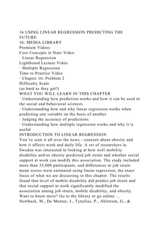
  • 4. Prediction is the computation of future outcomes based on a knowledge of present ones. When we want to predict one variable from another, we need to first compute the correlation between the two variables. Table 16.1 shows the data we will be using in this example. Figure 16.1 shows the scatterplot (see Chapter 5) of the two variables that are being computed. Table 16.1 ⬢ Total High School GPA and First-Year College GPA High School GPA First-Year College GPA 3.50 3.30 2.50 2.20 4.00 3.50 3.80 2.70 2.80 3.50 1.90 2.00 3.20 3.10 3.70 3.40 2.70 1.90 3.30 3.70 Figure 16.1 ⬢ Scatterplot of high school GPA and college GPA To predict college GPA from high school GPA, we have to create a regression equation and use that to plot what is called a regression line. A regression line reflects our best guess as to what score on the Y variable (college GPA) would be predicted
  • 5. by a score on the X variable (high school GPA). For all the data you see in Table 16.1, the regression line is drawn so that it minimizes the distance between itself and each of the points on the predicted (Y′) variable. You’ll learn shortly how to draw that line, shown in Figure 16.2. What does the regression line you see in Figure 16.2 represent? First, it’s the regression of the Y variable on the X variable. In other words, Y (college GPA) is being predicted from X (high school GPA). This regression line is also called the line of best fit. The line fits these data because it minimizes the distance between each individual point and the regression line. Those distances are errors because it means the prediction was wrong; it was some distance from the right answer. The line is drawn to minimize those errors. For example, if you take all these points and try to find the line that best fits them all at once, the line you see in Figure 16.2 is the one you would use. Second, it’s the line that allows us our best guess (at estimating what college GPA would be, given each high school GPA). For example, if high school GPA is 3.0, then college GPA should be around (remember, this is only an eyeball prediction) 2.8. Take a look at Figure 16.3 to see how we did this. We located the predictor value (3.0) on the x-axis, drew a perpendicular line from the x-axis to the regression line, then drew a horizontal line to the y-axis, and finally estimated what the predicted value of Y would be. Figure 16.3 ⬢ Estimating college GPA given high school GPA Third, the distance between each individual data point and the regression line is the error in prediction—a direct reflection of the correlation between the two variables. For example, if you look at data point (3.3, 3.7), marked in Figure 16.4, you can see that this (X, Y) data point is above the regression line. The distance between that point and the line is the error in prediction, as marked in Figure 16.4, because if the prediction were perfect, then all the predicted points would fall where? Right on the regression or prediction line.
  • 6. Figure 16.4 ⬢ Prediction is rarely perfect: estimating the error in prediction Fourth, if the correlation were perfect (and the x-axis meets the y-axis at Y ’s mean), all the data points would align themselves along a 45° angle, and the regression line would pass through each point (just as we said earlier in the third point). Given the regression line, we can use it to precisely predict any future score. That’s what we’ll do right now—create the line and then do some prediction work.CORE CONCEPTS IN STATS VIDEOLinear RegressionDRAWING THE WORLD’S BEST LINE (FOR YOUR DATA) The simplest way to think of prediction is that you are determining the score on one variable (which we’ll call Y— the criterion or dependent variable) based on the value of another score (which we’ll call X—the predictor or independent variable). The way that we find out how well X can predict Y is through the creation of the regression line we mentioned earlier in this chapter. This line is created from data that have already been collected. The equations are then used to predict scores using a new value for X, the predictor variable. Formula 16.1 shows the general formula for the regression line, which may look familiar because you may have used something very similar in a high school or college math course. In geometry, it’s the formula for any straight line: (16.1) Y'=bX+a,Y′=bX+a, where · Y ′ is the predicted score of Y based on a known value of X; · b is the slope, or direction, of the line; · X is the score being used as the predictor; and · a is the point at which the line crosses the y-axis. Let’s use the same data shown earlier in Table 16.1, along with a few more calculations that we will need thrown in.
  • 9. From this table, we see that · ∑ X, or the sum of all the X values, is 31.4. · ∑Y, or the sum of all the Y values, is 29.3. · ∑ X 2, or the sum of each X value squared, is 102.5. · ∑ Y 2, or the sum of each Y value squared, is 89.99. · ∑ XY, or the sum of the products of X and Y, is 94.75. Formula 16.2 is used to compute the slope of the regression line (b in the equation for a straight line): (16.2) b=ΣXY−(ΣXΣY/n)ΣX2−[(ΣX)2/n].b=ΣXY−(ΣXΣY/n)ΣX2−[(ΣX) 2/n]. In Formula 16.3, you can see the computed value for b, the slope of the line: (16.3) b=94.75−[(31.4×29.3)/10]102.5−[(31.4)2/10],b=2.7493.904=0.7 04.b=94.75−[(31.4×29.3)/10]102.5−[(31.4)2/10],b=2.7493.904= 0.704. Formula 16.4 is used to compute the point at which the line crosses the y-axis (a in the equation for a straight line): (16.4) a=ΣY−bΣXn.a=ΣY−bΣXn. In Formula 16.5, you can see the computed value for a, the intercept of the line: (16.5) a=29.3−(0.704×31.4)10,a=7.1910=0.719.a=29.3−(0.704×31.4)10 ,a=7.1910=0.719. Now, if we go back and substitute b and a into the equation for a straight line (Y = bX + a), we come up with the final regression line: Y'=0.704X+0.719.Y′=0.704X+0.719. Why the Y ′ and not just a plain Y ? Remember, we are using X to predict Y, so we use Y ′ to mean the predicted and not the actual value of Y. So, now that we have this equation, what can we do with it? Predict Y, of course. For example, let’s say that high school GPA equals 2.8 (or X =
  • 10. 2.8). If we substitute the value of 2.8 into the equation, we get the following formula: Y'=0.704(2.8)+0.719=2.69.Y′=0.704(2.8)+0.719=2.69. So, 2.69 is the predicted value of Y (or Y ′) given X is equal to 2.8. Now, for any X score, we can easily and quickly compute a predicted Y score. You can use this formula and the known values to compute predicted values. That’s most of what we just talked about. But you can also plot a regression line to show how well the scores (what you are trying to predict) actually fit the data from which you are predicting. Take another look at Figure 16.2, the plot of the high school–college GPA data. It includes a regression line, which is also called a trend line. How did we get this line? Easy. We used the same charting skills you learned in Chapter 5 to create a scatterplot; then we selected Add Fit Line in the SPSS Chart Editor. Poof! Done! You can see that the trend is positive (in that the line has a positive slope) and that the correlation is .6835—very positive. And you can see that the data points do not align directly on the line, but they are pretty close, which indicates that there is a relatively small amount of error. Not all lines that fit best between a bunch of data points are straight. Rather, they could be curvilinear, just as you can have a curvilinear relationship between your variables, as we discussed in Chapter 5. For example, the relationship between anxiety and performance is such that when people are not at all anxious or very anxious, they don’t perform very well. But if they’re moderately anxious, then performance can be enhanced. The relationship between these two variables is curvilinear, and the prediction of Y from X takes that into account. Dealing with curvilinear relationships is beyond the scope of this book, but fortunately, most relationships you’ll see in the social sciences are essentially linear. HOW GOOD IS YOUR PREDICTION? How can we measure how good a job we have done predicting one outcome from another? We know that the higher the
  • 11. absolute magnitude of the correlation between two variables, the better the prediction. In theory, that’s great. But being practical, we can also look at the difference between the predicted value (Y ′) and the actual value (Y) when we first compute the formula of the regression line. For example, if the formula for the regression line is Y ′ = 0.704X + 0.719, the predicted Y (or Y ′) for an X value of 2.8 is 0.704(2.8) + 0.719, or 2.69. We know that the actual Y value that corresponds to an X value is 3.5 (from the data set shown in Table 16.1). The difference between 3.5 and 2.69 is 0.81, and that’s the size of the error in prediction. Another measure of error that you could use is the coefficient of determination (see Chapter 5), which is the percentage of error that is reduced in the relationship between variables. For example, if the correlation between two variables is .4 and the coefficient of determination is 16% or .42, the reduction in error is 16% since initially we suspect the relationship between the two variables starts at 0 or 100% error (no predictive value at all). If we take all of these differences, we can compute the average amount that each data point differs from the predicted data point, or the standard error of estimate. This is a kind of standard deviation that reflects average error along the line of regression. The value tells us how much imprecision there is in our estimate. As you might expect, the higher the correlation between the two values (and the better the prediction), the lower this standard error of estimate will be. In fact, if the correlation between the two variables is perfect (either +1 or −1), then the standard error of estimate is zero. Why? Because if prediction is perfect, all of the actual data points fall on the regression line, and there’s no error in estimating Y from X. The predicted Y ′, or dependent variable, need not always be a continuous one, such as height, test score, or problem-solving skills. It can be a categorical variable, such as admit/don’t admit, Level A/Level B, or Social Class 1/Social Class 2. The score that’s used in the prediction is “dummy coded” to be a 0
  • 12. or a 1 (or any two values) and then used in the same equation. Yes, you are right that the level of measurement for this sort of correlational stuff is supposed to be at the interval level, but a variable with just two values works mathematically as if it has equal-sized intervals because there is only one interval. USING SPSS TO COMPUTE THE REGRESSION LINE Let’s use SPSS to compute the regression line that predicts Y′ from X. The data set we are using is Chapter 16 Data Set 1. We will be using the number of hours of training to predict how severe injuries will be if someone is injured playing football. There are two variables in this data set: Variable Definition Training (X) Number of hours per week of strength training Injuries (Y) Severity of injuries on a scale from 1 to 10 Here are the steps to compute the regression line that we discussed in this chapter. Follow along and do it yourself. 1. Open the file named Chapter 16 Data Set 1. 2. Click Analyze → Regression → Linear. You’ll see the Linear Regression dialog box shown in Figure 16.5. 3. Click on the variable named Injuries and then move it to the Dependent: variable box. It’s the dependent variable because its value depends on the value of number of hours of training. In other words, it’s the variable being predicted. 4. Click on the variable named Training and then move it to the Independent(s): variable box. 5. Click OK, and you will see the partial results of the analysis, as shown in Figure 16.6. We’ll get to the interpretation of this output in a moment. First, let’s have SPSS overlay a regression line on the scatterplot for these data like the one you saw earlier in Figure 16.2. 6. Click Graphs → Legacy Dialogs → Scatter/Dot. 7. Click Simple Scatter and then click Define. You’ll see the
  • 13. simple Scatterplot dialog box. 8. Click Injuries and move it to the variable label to the Y Axis: box. Remember, the predicted variable is represented by the y- axis. 9. Click Training and move it to the variable label to the X Axis: box. 10. Click OK, and you will see the scatterplot as shown in Figure 16.7. Now let’s draw the regression line. 11. If you are not in the chart editor, double-click on the chart to select it for editing. 12. Click on the Add Fit Line at Total button (on the second row of buttons, about fifth from the left) that looks a little like this: . 13. Close the Properties box that opened when you selected the Add Fit Line at Total button and then close the chart editor window. The completed scatterplot, with the regression line, is shown in Figure 16.8 along with the multiple regression value R2, which equals 0.21. As you will read more about shortly, the multiple regression correlation coefficient is the regression of all the X values on the predicated value. When you have the Properties dialog box open for drawing the regression line, notice that there is a set of Confidence Intervals options. When clicked, these show you a boundary within which there is a specific probability as to how good the prediction is. For example, if you click Mean and specify 95%, the graph will show you the boundaries surrounding the regression line, within which there is a 95% chance of the predicted scores occurring. This idea of wanting to be within a certain range of error 95% of the time is the same as wanting a .05 significance level for statistical analyses. Figure 16.5 ⬢ Linear Regression dialog box Understanding the SPSS Output The SPSS output tells us several things: 1. The formula for the regression line is taken from the first set of output shown in Figure 16.6 as Y ′ = –0.125X + 6.847. This
  • 14. equation can be used to predict level of injury given any number of hours spent in strength training. 2. As you can see in Figure 16.8, the regression line has a negative slope, reflecting a negative correlation (of –.458, which is what Beta is in Figure 16.6) between hours of training and severity of injuries. So it appears, given the data, that the more one trains, the fewer severe injuries occur. 3. You can also see that the prediction is significant—in other words, predicting Y from X is based on a significant relationship between the two variables such that the test of significance for both the constant (Training) and the predicted variable (Injuries) is significantly different from zero (which it would be if there was no predictive value for X predicting Y). So just how good is the prediction? Well, the SPSS output (which we did not show you) also indicates that the standard error of estimate for Injuries (the predicted variable) is 2.182; double that (4.36) and you’ll see that there is a 95% chance (remember 1.96 or about 2 standard deviations away from the mean creates a 95% confidence interval) the prediction will fall between the mean of all injuries (which is 4.33) and ±4.46. So, based on the correlation coefficient, the prediction is okay but not great. THE MORE PREDICTORS THE BETTER? MAYBE All of the examples that we have used so far in the chapter have been for one criterion or outcome measure and one predictor variable. There is also the case of regression where more than one predictor or independent variable is used to predict a particular outcome. If one variable can predict an outcome with some degree of accuracy, then why couldn’t two do a better job? Maybe so, but there’s a big caveat—read on. For example, if high school GPA is a pretty good indicator of college GPA, then how about high school GPA plus number of hours of extracurricular activities? So, instead of Y'=bX+a,Y′=bX+a, the model for the regression equation becomes Y'=bX1+bX2+a,Y′=bX1+bX2+a,
  • 15. where · X1 is the value of the first independent variable, · X2 is the value of the second independent variable, · b is the regression weight for that particular variable, and · a is the intercept of the regression line, or where the regression line crosses the y-axis. As you may have guessed, this model is called multiple regression (multiple predictors, right?). So, in theory anyway, you are predicting an outcome from two independent variables rather than one. But you want to add additional predictor variables only under certain conditions. Read on. LIGHTBOARD LECTURE VIDEO Multiple Regression Any variable you add has to make a unique contribution to understanding the dependent variable. Otherwise, why use it? What do we mean by unique? The additional variable needs to explain differences in the predicted variable that the first predictor does not. That is, the two variables in combination should predict Y better than any one of the variables would do alone. In our example, level of participation in extracurricular activities could make a unique contribution. But should we add a variable such as the number of hours each student studied in high school as a third independent variable or predictor? Because number of hours of study is probably highly related to high school GPA (another of our predictor variables, remember?), study time probably would not add very much to the overall prediction of college GPA. We might be better off looking for another variable (such as ratings on letters of recommendation) rather than collecting the data on study time. Take a look at Figure 16.9, which is the result of a multiple regression analysis that adds the number of extracurricular activity hours to the data you saw in Table 16.1. You can see how both high school GPA and number of hours of extracurricular activity are significant contributors to first-year college GPA. This is a powerful way of examining what and
  • 16. how more than one independent variable contribute to prediction of another variable. Figure 16.9 ⬢ A multiple regression analysis The Big Rule(s) When It Comes to Using Multiple Predictor Variables If you are using more than one predictor variable, try to keep the following two important guidelines in mind: 1. When selecting a variable to predict an outcome, select a predictor variable (X) that is related to the criterion variable (Y). That way, the two share something in common (remember, they should be correlated). 2. When selecting more than one predictor variable (such as X1 and X2), try to select variables that are independent or uncorrelated with one another but are both related to the outcome or predicted (Y) variable. In effect, you want only independent or predictor variables that are related to the dependent variable and are unrelated to each other. That way, each one makes as distinct a contribution as possible to predicting the dependent or predicted variable. There are whole books on multiple regression, and much of what one needs to learn about this powerful procedure is beyond the scope of this book. Chapter 18 talks more about multiple regression. How many predictor variables are too many? Well, if one variable predicts some outcome, and two are even more accurate, then why not three, four, or five predictor variables? In practical terms, every time you add a variable, an expense is incurred. Someone has to go collect the data, it takes time (which is $$$ when it comes to research budgets), and so on. From a theoretical sense, there is a fixed limit on how many variables can contribute to an understanding of what we are trying to predict. Remember that it is best when the predictor or independent variables are independent or unrelated to each other. The problem is that once you get to three or four variables, fewer things can remain unrelated.
  • 17. Better to be accurate and conservative than to include too many variables and waste money and the power of prediction. Real-World Stats How children feel about what they do is often very closely related to how well they do what they do. The aim of this study was to analyze the consequences of emotion during a writing exercise. In the model this research follows, motivation and affect (the experience of emotion) play an important role during the writing process. Fourth and fifth graders were instructed to write autobiographical narratives with no emotional content, positive emotional content, and negative emotional content. The results showed no effect regarding these instructions on the proportion of spelling errors, but the results did reveal an effect on the length of narrative the children wrote. A simple regression analysis (just like the ones we did and discussed in this chapter) showed a correlation and some predictive value between working memory capacity and the number of spelling errors in the neutral condition only. Since the model on which the researchers based much of their preliminary thought about this topic states that emotions can increase the cognitive load or the amount of “work” necessary in writing, that becomes the focus of the discussion in this research article. Want to know more? Go online or to the library and find … Fartoukh, M., Chanquoy, L., & Piolat, A. (2012). Effects of emotion on writing processes in children. Written Communication, 29, 391–411. Summary Prediction is a useful application of simple correlation, and it is a very powerful tool for examining complex relationships. This chapter might have been a little more difficult than others, but you’ll be well served by what you have learned, especially if you can apply it to the research reports and journal articles that you have to read. We are now at the end of lots of chapters on inference, and we’re about to move on in the next part of this book to using statistics when the sample size is very small or when the assumption that the scores are distributed in a normal
  • 18. way is violated. Time to Practice 1. How does linear regression differ from analysis of variance? 2. Chapter 16 Data Set 2 contains the data for a group of participants who took a timed test. The data are the average amount of time the participants took on each item (Time) and the number of guesses it took to get each item correct (Correct). a. What is the regression equation for predicting response time from number correct? b. What is the predicted response time if the number correct is 8? c. What is the difference between the predicted and the actual number correct for each of the predicted response times? Time to Practice Video Chapter 16: Problem 2 Chapter 16, Problem 2 will show you how to compute a linear regression, so you can answer the question about the regression equation and make some predictions. Doing a regression is pretty straightforward. First, we want to go to our SPSS Data Set, which is Chapter 16, Data Set 2. Once we're here, we want to go to Analyze, then Regression, then Linear, since we're using just two variables. When we click on Linear, you want to think about where you place your dependent and independent variables. The dependent is the outcome, or that thing that is dependent on something else. In this case, the number of correct answers is dependent on the amount of time we think they spent on it. So, correct answers is the dependent and time is the independent. Click OK, and our output pops up. The key thing we're going to look at for making the prediction is under Coefficients. And, for doing this, we're going to look at the Unstandardized Beta Weights. Here you see 7.414 and negative This is the two bits of information. So let's refresh ourselves with what the data set looks like in terms of creating a regression equation. This is the regression equation. And so, what we have already, we figured out the beta and then we figured out the point at which it crosses the
  • 19. y-axis. When we put that information here, here is our regression equation, y equals negative So, that's the equation for Part A. Part B asks us to make a prediction. What is the predicted time if the number of correct answers is 8? In this situation, we take our regression equation, but now we add the x, in this case 8, the number of correct answers, we do the computation, and we come up with 6.262, which is the predicted time. Part C asks you to determine the difference between the predicted and actual time for each of them. And then all you want to do there is, when you look at your data set, is take the predicted and compute that, but instead of putting in 8, put in each of these numbers, and come up and compute the difference. And that's how we answer Chapter 16, Problem 2. Good luck. 1. Betsy is interested in predicting how many 75-year-olds will develop Alzheimer’s disease and is using as predictors level of education and general physical health graded on a scale from 1 to 10. But she is interested in using other predictor variables as well. Answer the following questions: a. What criteria should she use in the selection of other predictors? Why? b. Name two other predictors that you think might be related to the development of Alzheimer’s disease. c. With the four predictor variables—level of education and general physical health and the two new ones that you named in (b)—draw out what the model of the regression equation would look like. 2. Go to the library or online and locate three different research studies in your area of interest that use linear regression. It’s okay if the studies contain more than one predictor variable. Answer the following questions for each study: a. What is one independent variable? What is the dependent variable? b. If there is more than one independent variable, what argument does the researcher make that these variables are independent of one another?
  • 20. c. Which of the three studies seems to present the least convincing evidence that the dependent variable is predicted by the independent variable, and why? 3. Here’s where you can apply the information in one of this chapter’s tips and get a chance to predict a Super Bowl winner! Joe Coach was curious to know whether the average number of games won in a year predicts Super Bowl performance (win or lose). The X variable was the average number of games won during the past 10 seasons. The Y variable was whether the team ever won the Super Bowl during the past 10 seasons. Here are the data: Team Average Number of Wins Over 10 Years Bowl? (1 = yes and 0 = no) Savannah Sharks 12 1 Pittsburgh Pelicans 11 0 Williamstown Warriors 15 0 Bennington Bruisers 12 1 Atlanta Angels 13 1 Trenton Terrors 16 0 Virginia Vipers 15 1 Charleston Crooners
  • 21. 9 0 Harrisburg Heathens 8 0 Eaton Energizers 12 1 a. How would you assess the usefulness of the average number of wins as a predictor of whether a team ever won a Super Bowl? b. What’s the advantage of being able to use a categorical variable (such as 1 or 0) as a dependent variable? c. What other variables might you use to predict the dependent variable, and why would you choose them? 4. Check your calculation of the correlation coefficient of the relationship between coffee consumption and stress done in Chapter 15, Question 5. If you want to know whether coffee consumption predicts group membership: a. What is the predictor or the independent variable? b. What is the criterion or the dependent variable? c. Do you have an idea what R2 will be? 5. Time to try out multiple predictor variables. Take a look at the data shown here where the outcome is becoming a great chef. We suspect that variables such as number of years of experience cooking, level of formal culinary education, and number of different positions (sous chef, pasta station, etc.) all contribute to rankings or scores on the Great Chef Test. By this time, you should be pretty much used to creating equations from data like these, so let’s get to the real questions: Years of Experience Level of Education # Positions Score on Great Chef Test 5 1
  • 24. 16 88 a. Which are the best predictors of a chef’s score? b. What score can you expect from a person with 12 years of experience and a Level 2 education who has held five positions? 6. Take a look at Chapter 16 Data Set 3, where number of home sales (Number_Homes_Sold) is being predicted by years in the business (Years_In_Business) and level of education in years (Level_Of_Education). Why is level of education such a poor contributor to the overall prediction (using both years in the business and level of education combined) of number of homes sold? What’s the best predictor and how do you know? (Hint: These are sort of trick questions. Before you go ahead and analyze the data, look at the raw data in the file for the characteristics you know are important for one variable to be correlated with another.) 7. For any combinations of predicted and predictor variables, what should be the nature of the relationship between them? Student Study Site Get the tools you need to sharpen your study skills! Visit edge.sagepub.com/salkindfrey7e to access practice quizzes, eFlashcards, original and curated videos, data sets, and more! Chapter 9 Global Inequality and Poverty ONE PHOTO CAPTURES A SHARP CONTRAST BETWEEN RICH AND POOR IN THE DEVELOPING WORLD. The high- rise buildings in the background are apartments for the wealthy. Learning Objectives 1. 9.1Examine how widening gap between rich and poor strengthens inequality-perpetuating institutions 2. 9.2Contrast between the viewpoints of globalists and antiglobalists on the effects of globalization
  • 25. 3. 9.3Examine the causes and the impact of domestic or global inequality between nations 4. 9.4Examine the economic, social, and educational inequality that exists within rich countries 5. 9.5Examine the inequalities that exist in different aspects of life in poor countries 6. 9.6Review the six dimensions of poverty that can be used to gauge poverty 7. 9.7Evaluate some of the measures for diminishing poverty and reducing inequality The richest eighty people in the world control as much wealth as the poorest half of the world’s population. Thirty-five of those eighty are Americans. The top 1 percent of the world’s richest people control 48 percent of the world’s total wealth. More than one billion people in the world live on less than $1.25 a day.1 Inequality exists within the United States. The richest four hundred Americans own more assets than the poorest 150 million, or almost half the population. The bottom 15 percent, about forty-six million people, live in households earning less than $22,000 per year. The top 5 percent of households in Washington, D.C., make an average of more than $500,000, while the bottom 20 percent make less than $9,500. Conflict between rich and poor is now the greatest source of tension in American society. Economic inequality has emerged as a dominant global issue that has fueled massive protests and popular uprisings. The global financial crisis and economic recession have rekindled debates about inequality and its consequences. Discussions about wealth and poverty and how to achieve greater equality are as old as human society. They demonstrate a perennial concern about the implications of inequality for the security and well-being of communities. Given the persistence of inequality among individuals, groups, and nations over centuries, this debate is interminable. Struggles to achieve equality are also endless. Issues pertaining to global inequality and poverty permeate almost every significant global problem, from trade to the environment, from
  • 26. terrorism and criminal activities to democratization and human rights, and from ethnic conflicts to the proliferation of weapons of mass destruction. As we have seen, popular uprisings in the Middle East and North Africa were strongly influenced by widespread inequality and poverty. Consequently, as our discussion shows, inequality and poverty are closely connected to politics, economics, and culture. A central question addressed in this chapter is whether inequality matters. Human societies are inherently unequal due to variations of abilities, opportunities, geographic location, luck, personal characteristics, and so on. But why is it important to address issues of inequality, something that societies have struggled with historically? Globalization is widely perceived as the major cause of global inequality. Yet, as we have noted, unequal distributions of wealth existed independent of the current wave of globalization and are present in societies little affected by it. This chapter analyzes the globalization and inequality debate as well as the current state of global inequality. In addition to focusing on inequality between rich and poor countries and inequality within both developed and developing societies, we will examine the issue of gender inequality. This chapter discusses the enduring issues of global poverty, hunger and malnutrition, economic development and poverty, and efforts to close the gap between rich and poor and reduce the negative effects of inequality and poverty. The chapter concludes with a case study of food security and rising food prices.9.1: Does Inequality Matter? 1. 9.1 Examine how widening gap between rich and poor strengthens inequality-perpetuating institutions The existence of inequality is not automatically a major problem, especially when the economy is growing and there are many opportunities for upward mobility. As long as the standard of living is improving for those on the bottom of the economic ladder, concerns about inequality tend to diminish. The last two decades of the twentieth century and the first decade of this century were characterized by a widening gap between rich and
  • 27. poor and the proliferation of millionaires and billionaires. While economic disparities remained a serious problem in developing countries, the forces of globalization created conditions that helped widen the gap between rich and poor in industrialized societies. When the economy deteriorates, the gap between rich and poor tends to be narrower, but concerns about inequality are heightened. During the global economic recession, the wealthy lost money, but the poor lost their jobs, houses, and health insurance. In the United States, the poverty rate peaked at 15.1 percent in 2010, its highest level since 1993. In 2013, the poverty rate was still high, at 15.0 percent. Widespread demonstrations in the United States against excessive executive compensation, especially those in companies that received financial assistance from the government, underscores the dangers of economic inequality. The financial and economic crisis increased inequality and heightened awareness of the concentration of wealth held by the top 1 percent of Americans. That awareness led to “We are the 99 percent,” a battle cry of the Occupy Wall Street protests against financial inequality that began in New York City and spread around the world. The perception that economic inequality is essentially transitory when opportunities for economic advancement are widely available mitigates negative effects of actual inequality. However, persistent inequality and enduring poverty challenge beliefs in the equality of opportunity and the possibility of upward mobility. Eventually, the legitimacy of the economic system and political and social institutions are challenged. Extreme inequality is detrimental to sustainable economic growth. The legitimacy of the global economic system is likely to be strengthened if a larger number of countries and individuals are benefiting from it. Extreme inequality perpetuates poverty and the concentration of economic and political power and reduces economic efficiency. It strengthens inequality-perpetuating institutions in three ways:
  • 28. 1. Inequality discourages the political participation of poor people, which, in turn, diminishes their access to education, health care, and other services that contribute to economic growth and development. 2. Inequality often prevents the building and proper functioning of impartial institutions and observance of the rule of law. 3. Inequality enables the wealthy to refuse to compromise politically or economically, which further weakens poor societies in a global society that requires relatively fast responses to economic developments.2 These consequences of inequality combine to ensure that poor societies will remain poor and unequal, trapping most of their inhabitants in a destructive cycle of poverty. Growing inequality among as well as within nations has direct and indirect implications for globalization. Inequality could undermine globalization by influencing countries to adopt protectionist policies and disengage, to the extent possible, from the global economy. But the ramifications extend beyond economic issues to problems such as terrorism, the environment, and the spread of infectious diseases. Inequality influences global perceptions of America and weakens its soft power, or its cultural attraction. As Chapter 4 shows, the democratization process and the effective functioning of consolidated democracy depend largely on a significant degree of economic and social equality. The legitimacy of any democratic system is contingent upon the voters’ belief that they have a vested interest in its preservation. Their allegiance to the democracy is influenced partly by the benefits they derive from the economic system. Inequality undermines democracy by fostering despair and alienation among workers and corruption and the abuse of power among the wealthy. It corrodes trust and civility among citizens. Inequality destroys the people’s will to engage in collective solutions to political, social, and economic problems because it weakens their sense of unity and common interests. Massive protests globally against governments underscore this point.
  • 29. The unequal distribution of wealth is often mitigated by government redistributive policies. Extreme inequality sometimes results in the voters pressuring governments to enact trade protection legislation to safeguard their employment and livelihoods. In this case, voters exercising their democratic rights could inadvertently undermine the economic system that supports democracy. Global and domestic inequalities often directly affect many areas. Terrorism is widely linked to poverty within developing nations. Huge inequalities often fuel resentment, which finds expression in global crime and a general disregard for the rules and norms of global society. Those who are extremely poor are often excluded from participation in decisions that negatively impact their lives. They become vulnerable to being influenced by radical minorities who are committed to violent change. Poverty contributes to global and regional problems by fueling ethnic and regional conflicts, creating large numbers of refugees, and inhibiting access to resources, such as petroleum. Finally, global and domestic inequality is perceived as stimulating the global drug trade. For example, poor farmers in Bolivia regard the cultivation of coca as essential to their survival. More than three-quarters of the heroin sold in Europe is refined from opium grown in Afghanistan by poor farmers. The costs of fighting the war against drugs in poor countries, such as Colombia and Afghanistan, are extremely high.9.2: The Globalization and Inequality Debate 1. 9.2 Contrast between the viewpoints of globalists and antiglobalists on the effects of globalization The impact of globalization on income distribution and living standards is a controversial topic. Preoccupation with globalization to the exclusion of other factors often muddles the debate about globalization and inequality. Would less globalization produce more equality, and would more equality among and within nations result in an improved quality of life for the poor? There are two dominant, but sometimes overlapping, viewpoints on this issue. The globalists argue that
  • 30. globalization has increased economic growth and decreased global inequality and poverty. The antiglobalists generally perceive globalization as a negative and destructive force that is responsible for the increasing global inequality and poverty and the declining levels of human welfare.39.2.1: Globalists Make Their Case From the globalists’ perspective, the basic cause of inequality and poverty is the relatively low level of globalization in some countries. In other words, the poorest societies are the least integrated into the global economy. Openness to foreign trade, investments, and technology—combined with reforms such as the privatization of the domestic economy—will ultimately accelerate economic growth. The Organization for Economic Cooperation and Development (OECD) calculated that countries that are relatively open to trade grew about twice as fast as those that are relatively closed to trade.4 China’s rapid economic growth is an obvious example. On the other hand, North Korea, Myanmar (formerly Burma), and Kenya are on the margins of globalization and remain impoverished. Globalists also argue that globalization has contributed to the decline of inequality. Furthermore, poverty can be reduced even as inequality increases. David Dollar and Aart Kraay found that “a long-term global trend toward greater inequality prevailed for at least 200 years; it peaked around 1975. But since then, it has stabilized and possibly even reversed.”5 The accelerated economic growth of China and India, the world’s two most populous countries, which is seen as directly linked to globalization, is given as the principal reason for the change. Much of the inequality that persists within countries is due less to globalization and more to policies dealing with education, taxation, and social problems. Moreover, more economic growth in China, for example, has been accompanied by a spectacular reduction in poverty.6 Globalists emphasize that the number of people moving out of poverty has increased. More than 800 million people have abandoned the ranks of absolute poverty since 1990. The
  • 31. number of people living in absolute poverty remains high— around 1.2 billion. But given rapid population growth rates in the poorest countries, the decline in global poverty is impressive. The world’s poor are seen as getting to be less poor in both absolute and relative terms.7 The more globalized poor nations become, the better off their populations are in both absolute and relative terms. Globalization has generally helped the poor by contributing to reductions in the cost of numerous consumer products. Less money has higher purchasing power in a globalized economy. Finally, by facilitating migration, establishing small businesses that rely on the Internet, and improving access to jobs in telecommunications and computer technologies in countries such as India and China, globalization improves the quality of life for the poor.9.2.2: Antiglobalists Make Their Case Antiglobalists believe that globalization is widening the gap between the haves and the have-nots. Concerned with making global capitalism more equitable, they view globalization as primarily benefiting the rich while making life more difficult for the poor. Antiglobalists argue that globalization is a zero- sum game, meaning that the rich are winning at the expense of the poor. Antiglobalists also argue that globalization benefits rich countries, such as the United States. China is one of the few developing countries that is generally regarded as profiting from free trade and open markets. The United States, the locomotive of globalization, benefits the most from open markets worldwide. George Soros—a leading financier, philanthropist, and critic of globalization, though not an antiglobalist—believes that globalization drains surplus capital from periphery or developing countries to the United States, thereby allowing Americans to spend more than they save and import more than they export.8 Similarly, Jack Beatty contends that the foundation of inequality resulting from globalization is that rich countries do not play by the rules that they made to govern the global economic system. Basically, the United States and other Western countries require developing countries to
  • 32. open their markets without reciprocating commensurably. To support this argument, Beatty points out that although global rules on trade discourage governments from subsidizing industries, rich countries continue to provide subsidies to agriculture.9 Critics also argue that globalization is like an “economic temptress,” promising riches but not delivering. Global communications have heightened awareness of the vast disparities between rich and poor within the same society and especially between rich and poor countries. Simultaneously, global communications spawn aspirations of escaping poverty and enjoying the good life. Unfortunately, globalization is unable to make these dreams real. Countries integrated into the global economic system are the most severely affected by downturns in the economy. For example, Southeast Asia, which depends on exports of steel, textiles, and electronic components, suffers significantly in global economic crises and is unable to generate enough jobs and sufficient wages for a population with aspirations nurtured by television programs that depict prosperity. Although conceding that globalization is not entirely responsible for global poverty, antiglobalists generally view globalization as a tide that lifts a few boats while leaving the majority mired at the bottom. Even when global companies create jobs within societies, the race to the bottom in labor standards and wages inevitably results in the poor in developing countries being unable to escape poverty while, at the same time, reducing the wages for workers in rich countries or depriving them of employment. This development is intertwined with the precipitous decline of private sector labor unions. Kim Phillips-Fein argues that unions mobilize their members to vote for government policies that help redistribute wealth and reinforce upward mobility, which strengthen the middle class.10 Antiglobalists contend that globalization compounds existing inequalities and creates more inequality. By giving priority to privatization, globalization weakens governments’ commitment to the public sector. Vito Tanzi states that “even as the forces of
  • 33. globalization boost the demand for strong social safety nets to protect the poor, these forces also erode the ability of governments to finance and implement large-scale social welfare policies.”11 The emphasis on integrating poor nations into the global economy diverts resources from more urgent development needs, such as education, public health, industrial capacity, and social cohesion. Many trade agreements impose tight prerequisites on developing countries in exchange for crumbs of enhanced market access. The African Growth and Opportunity Act is an example. It provides increased access to the U.S. market only if African apparel manufacturers use fabric and yarns produced in the United States, instead of using their own or supplies from less expensive sources. In other words, the antiglobalists perceive globalization as perpetuating inequality by impeding development. Furthermore, they argue, countries such as South Korea and Taiwan, that globalists frequently held up as models for the benefits of globalization developed under radically different conditions. These countries were not required to pay the costs that are now an integral component of integration into global markets. During the 1960s and 1970s, when they were rapidly growing, Taiwan and South Korea did not face contemporary globalization’s pressures to privatize their economies and open their borders to capital flows. The demands of globalization undermine efforts essential for a comprehensive development agenda. 9.3: Global Inequality 1. 9.3 Examine the causes and the impact of domestic or global inequality between nations Discussions of global inequality remind us of many of the reasons some societies created powerful and prosperous civilizations while others did not. Western Europe emerged as the most prosperous region of the world. Areas that are now the United States, Canada, Australia, and New Zealand were conquered and settled by Europeans, many of whom embodied the characteristics that contributed to Europe’s rise to global
  • 34. prominence and economic prosperity. The advantages Europeans enjoyed have been consolidated. This, in turn, contributes to global inequality today. Several factors combined to produce Europe’s economic success and profound global economic inequality. A major factor is freedom of expression. Societies that encouraged people to have their own ideas, to be innovative, and to interact with each other eventually surpassed societies that were totalitarian or authoritarian. The latter generally stifled innovation because of their preoccupation with traditions, conformity, and respect for authority. Initiative was often equated with heresy. Another factor encompasses social values. Chief among these is an emphasis on economic opportunity and social equality. In his Wealth and Poverty of Nations, David S. Landes stresses that China’s restrictions on women hampered its growth, whereas women in Europe, who were less confined to the home and were free to find employment in certain occupations, were instrumental in that region’s industrial development and expansion.12 A third factor is the functioning of a free market and institutionalized property rights. Chinese authorities became antagonistic toward free enterprise and eventually regulated it out of existence. Muslim countries failed to develop institutions that would have enabled businesses to expand. Islamic partnership law and inheritance law worked against the growth of large corporations. In Europe, a partner in a business could designate heirs, thereby providing continuity in the business after the partner’s death. Islamic law did not provide mechanisms for partnerships to be easily reconstituted following a partner’s death. Similarly, Islamic law prescribed in rigid detail both immediate and extended family members who had to inherit property. Europe, on the other hand, allowed property to be inherited by one person, thereby minimizing the chances that a business would disintegrate and be prevented from getting larger. Virginia Postrel points out that “the fragmentation produced by inheritance law, combined with the structures of partnership law, kept Middle Eastern enterprises small. That, in turn, limited the pressure to evolve
  • 35. new economic forms.”13 However, increasing wealth from petroleum has significantly strengthened many companies in the Persian Gulf area, especially those involved in finance. A final factor undergirding Europe’s economic success and setting the foundation for global inequality is the separation of the secular from the religious. Whereas Islam became inseparable from the state, the origins of Christianity and its spread to Rome forced it to compromise with secular authority, a compromise encapsulated in the warning that Christians should give to Caesar what belongs to him and give God what is God’s. However, Muslim societies prospered when religion was less restrictive. Muslims, commanded by the Koran to seek knowledge, became leading scientists, physicians, artists, mathematicians, philosophers, architects, and builders. For more than five hundred years, Arabic was the language of scholars and scientists. Muslims transmitted Chinese scientific inventions, Greek and Persian texts, and their own impressive scientific discoveries and inventions to Europe. From the tenth to the thirteenth centuries, Europeans translated Arabic works into Hebrew and Latin, thereby giving impetus to a rebirth of learning that ultimately transformed Western civilization. 9.3.1: Inequality between Developed and Developing Countries Despite rising living standards throughout most of the world, the gap between rich and poor countries has steadily widened. Tables 9.1 and 9.2 show some of those disparities in greater detail. Historic trends suggest that most of the richest countries will maintain their lead over most of the poorest countries. The gap between the richest country and the poorest country was 3 to 1 in 1820, 11 to 1 in 1913, 35 to 1 in 1950, 44 to 1 in 1973, and 72 to 1 in 1992. By the end of the twentieth century, the richest 20 percent of the world’s population had eighty-six times as much income as the poorest 20 percent. At the beginning of the twenty-first century, the average income in the richest twenty Table 9.1 Income Inequality among Countries, 2011 (in terms of GDP per capita)
  • 36. Adapted from UN Development Programme, Human Development Report 2013: The Rise of the South. Human Progress in a Diverse World (New York: UN Development Program, 2013). GDP per capita is given in international dollars using purchasing power parity rates (PPP). Some Rich Countries Qatar 77,987 Luxembourg 68,458 Singapore 53,591 Norway 46,982 Brunei Darussalam 45,507 Hong Kong, China (SAR) 43,844 United States 42,486 United Arab Emirates 42,293 Switzerland 37,979 Netherlands 37,251 Australia 34,548 Japan 30,660 Republic of Korea (South Korea) 27,541 Some Poor Countries Ethiopia 979
  • 37. Mali 964 Togo 914 Mozambique 861 Madagascar 853 Malawi 805 Sierra Leone 769 Central African Republic 716 Niger 642 Burundi 533 Eritrea 516 Liberia 506 Democratic Republic of the Congo 329 countries was thirty-seven times that in the poorest twenty countries.14 As Table 9.1 indicates, income disparities between developed and developing countries are very wide. Economic development, while dramatically improving the standard of living in most countries, has not significantly closed the gap because of differential growth rates between rich and poor countries. Rich countries have experienced higher economic growth rates than poor countries. Furthermore, per capita income actually declined in more than one hundred of the world’s poorest countries, many of them in Africa. Even developing countries that have enjoyed unprecedented economic growth, such as China and India, have failed to close the gap
  • 38. between themselves and rich countries. It is estimated that it would take China and India a hundred years of constant growth rates higher than those now experienced by industrialized countries just to reach current American income levels. However, given the extraordinarily high standard of living in the United States, both China and India would be relatively prosperous if they achieved half the income level of Americans. Furthermore, globalization is profoundly altering many old assumptions. Because the income gap between rich and poor countries has widened historically, it does not necessarily follow that this will always be the case. Singapore and Kuwait, two high-income countries, illustrate that poor countries can become prosperous by implementing astute political, social, and economic policies (in the case of Singapore) or by having valuable natural resources (in the case of Kuwait). Economic disparities between the developed and the developing world have focused on the global digital divide. But access to the Internet and improved telecommunications are not automatic panaceas for solving the problems of developing societies. 9.3.2: Causes of Inequality between Rich and Poor Countries In this section, we will briefly discuss some causes of the widening gap between rich and poor countries. It is important to remember that several factors combine to contribute to inequality: (1) geography, (2) colonialism and its legacies, (3) the structure of the global economy, (4) population growth, (5) government policies, (6) political instability, and (7) natural disasters. Geography Countries that are poor, some argue, have certain geographic characteristics that contribute to their economic problems. For example, they are in tropical regions or face high transportation costs in accessing global markets because of their location. Apart from the prevalence of tropical diseases, which have been controlled to a large extent by modern medicines and practices, countries in the Southern Hemisphere also tend to suffer from being landlocked. Countries with extensive coastlines and good
  • 39. harbors tend to be better off economically than landlocked countries that lack the physical infrastructure (i.e., systems such as roads and railroads) essential for gaining access to navigable rivers and the sea. Landlocked countries or countries located far from global markets are disadvantaged by high transportation costs. Colonialism Many argue that European colonization of Africa, Asia, and Latin America laid the foundation for economic disparities between rich and poor nations. Inequality breeds inequality. Just as wealth tends to perpetuate wealth, poverty tends to perpetuate poverty. Countries that grew rich two hundred years ago, partly because of their colonization of the developing world, are generally still rich today. European groups that migrated to Australia, Canada, the United States, South Africa, New Zealand, and throughout Latin America continue to enjoy significant advantages Table 9.2 Health Inequalities Adapted from UN Development Programme, Human Development Report 2013: The Rise of the South. Human Progress in a Diverse World (New York: UN Development Program, 2013). Physicians, 2005–2010 (per 1,000 people) Life Expectancy at Birth, 2012 (years) Maternal Mortality Ratio, 2010 (deaths per 100,000 live births) Country Rich Countries Norway 4.1
  • 41. 83.6 5 Republic of Korea (South Korea) 2.0 80.7 16 Poor Countries Guinea 0.1 54.5 610 Central African Republic 0.1 49.1 890 Burkina Faso 0.1 55.9 300 Democratic Republic of Congo 0.1 48.7 540 Sierra Leone 0.0 48.1 890 Burundi 0.0 50.9 800 Eritrea 0.0
  • 42. 62 240 Mali 0.0 51.9 540 Chad 0.0 49.9 1,100 Mozambique 0.0 50.7 490 Niger 0.0 55.1 590 over indigenous populations. However, it is also argued that colonization is not the main reason for ongoing global inequality. Some states, such as Singapore, South Korea, and Taiwan, that were colonized are now relatively rich. Structure of the Global Economy Colonialism and historical experiences, as well as contemporary economic practices, are widely perceived as creating an unfair global economy that keeps poor countries poor and rich countries rich. The Scottish economist Adam Smith, who wrote An Inquiry into the Nature and Causes of the Wealth of Nations, believed that governments should not interfere with the functioning of markets and that businesspersons would be led by an invisible hand to do the best for society. However, many leaders of poor countries argue that governments and multinational corporations in rich countries cooperate to maintain an unfair global economy. They generally subscribe to the dependency theory, which holds that poor countries’ reliance on exports of primary commodities, many of
  • 43. which were started during colonization for the benefit of Europeans, puts them at a severe economic disadvantage. The prices obtained from their exports decline relative to the prices of manufactured imports from industrialized countries. Population Growth Rapid population growth in most developing countries plays a central role in perpetuating the economic chasm between rich and poor countries. Population growth decreased in the industrialized countries as the economic gap was widening. Since 1950, the population in rich countries grew by about 50 percent. In sharp contrast, the population in poor countries grew by 250 percent. Large families perpetuate poverty in most cases. Government Policies Discussing causes of poverty in the Arab world, Alan Schwartz observed that many of these countries are poor because of the policies they pursue. For example, Saudi Arabia tolerates monopolies that help sustain an elite clan that all too often opposes technological, economic, and social change. Many Arab countries use import duties to discourage trade and impede the flow of investment by disregarding the rule of law. Furthermore, many of these governments emphasize religion instead of science and technology and therefore do not adequately develop human capital. Perhaps the most serious policy failure is the lack of adequate investment in women’s education and opposition to allowing women to have equal employment opportunities. When Korea was divided in 1948, South Korea adopted capitalist policies that fostered economic success, whereas North Korea isolated itself from the global community and adopted a Communist system of government. Today, South Korea is prosperous, and North Korea routinely faces starvation. China, India, Malaysia, and Singapore, for example, implemented policies that have a positive impact on their economies. Latin America, on the other hand, disproportionately allocates resources to the wealthy. Although several countries, especially Brazil, have made progress toward enlarging the middle class, many of the poor there remain
  • 44. trapped in the cycle of poverty.Political Instability Angola, a country twice the size of Texas, has abundant supplies of petroleum, diamonds, fish, and fresh water. However, life expectancy there is forty-five years, infant mortality is among the highest in the world, and Angolans are extremely poor. For twenty-seven years, the country was devastated by ethnic conflicts. Political instability directly contributes to economic disparities between developed and developing countries. Conflict not only discourages foreign investment, it also influences the best educated, most talented, and most financially successful citizens to flee or to invest their money outside the country.Natural Disasters At the beginning of this section, we discussed how geographic location directly affects the wealth and poverty of countries. Drought, earthquakes, volcanic eruptions, hurricanes, and other natural disasters are closely linked to geography. The earthquake and tsunami in Japan; tsunamis in Asia; Hurricanes Katrina, Rita, and Sandy in the United States; earthquakes in China; flooding in Pakistan; and Typhoon Haiyan in the Philippines are the most obvious examples. These natural disasters routinely destroy important economic sectors, increase severe infrastructure problems, force the relocation of a large number of people, and lead to greater impoverishment.9.4: Inequality Within Rich Countries 1. 9.4 Examine the economic, social, and educational inequality that exists within rich countries History and literature are replete with examples of the difficulties endured by the poverty-stricken citizens of Britain and the United States and how the lives of the poor sharply contrasted with those of the wealthy. Theories of socialism and Communism, articulated by Karl Marx, who was living in Britain, underscore the durability of inequality within rich countries. Great economic disparities have existed in the United States throughout its history, with the Gilded Age of the nineteenth century, the Roaring Twenties, and the Roaring Nineties bringing unprecedented levels of both prosperity and
  • 45. economic inequality. The stock market crash of 1929, the Great Depression of the 1930s, the implementation of the New Deal programs designed to help the poor, and the outbreak of World War II combined to redistribute wealth in the United States. The concentration of income declined dramatically, and the middle class grew rapidly. Income distribution remained relatively equal until the 1970s. In virtually all industrial countries, income inequality grew between the 1970s and the early twenty-first century. Globalization, new technologies, the financial crisis and economic recession, and other factors contributed to this development. Globalization is generally seen as a major cause of the rapid rise in inequality. Integral to globalization is the proliferation of new telecommunications and computer technologies. Individuals with technical skills have outperformed those who have few or no technical skills. The globalization of trade also contributed to shifting employment patterns, with low-wage workers in industrial countries losing out to workers in the developing world. Closely related to globalization and technology is education. The knowledge-based economies of rich countries give educated individuals an advantage over those who are less educated, less skilled, and less entrepreneurial. The interdependence of economies enables educated people to be more mobile and marketable. The new global elites are mainly entrepreneurs. Many of them are inventors in the area of communications technologies. The disparity in income between those with a high school education on the one hand and those with a college education on the other became obvious between 1979 and the early 1990s. In 1979, the average American male college graduate earned 49 percent more than a male high school graduate. By 1993, the gap had grown to 89 percent. The forces of globalization continue to widen this gap. Individuals with doctorates and professional graduate degrees experience significant income growth. The weakening of labor unions, as we discussed in Chapter 8, also contributes to rising inequality.9.4.1: The United States
  • 46. The United States has the greatest degree of income inequality among industrialized countries. The richest country on earth also has pockets of poverty that are similar to many parts of the developing world. In 2013, the poverty line was defined as an annual income below $22,314 for a family of four, and 15 percent of Americans—46.5 million people—lived below this line. The poorest 10 percent of Americans receive 1.8 percent of the total income, whereas the richest 10 percent get almost a third. The average for rich countries is 2.9 percent of the total income going to the poorest 10 percent of the population. Economic statistics support the general perception of unprecedented inequality in the United States, with most of the income concentrated at the very top of society. The top 20 percent of households earned 56 percent of the nation’s income and controlled 83 percent of the nation’s wealth, which includes stocks, bonds, real estate, businesses, savings, insurance, and other assets. Between 1980 and 2006, the top 1 percent of Americans earned ten times more than the rest at the start of the period and twenty times more than the rest at the end. The top 1 percent of earners take more than one-fifth of the income earned by Americans. For the top 0.1 percent, the gain rose from twenty times the earnings of the lower 90 percent to almost eighty times by 2006. The top 10 percent receive more than half of America’s total income and control half the nation’s wealth. The richest 400 Americans own more assets than the poorest 150 million, which is almost half the population. More than 90 percent of all income gains since 2009 have gone to the top 1 percent.15 The top 5 percent of households in Washington, D.C., made an average of more than $500,000, while the bottom 20 percent made around $9,500. The tax cuts passed in 2001 and 2003 were widely regarded as creating an even wider gap between the rich and poor in the United States. Perhaps one of the most overlooked aspects of inequality is the growing income gap between urban areas and rural America. As one drives through the numerous small towns in Illinois, Iowa,
  • 47. North Dakota, Alabama, and elsewhere, these income disparities become obvious. Homes, businesses, barns, and grain elevators have been abandoned and are decaying, creating what are referred to as rural ghettos. Two New York academics, Frank and Debra Popper, have suggested that given the relentless decay of rural towns, the federal government should accelerate the depopulation of the entire Great Plains region and turn it into a vast Buffalo Commons, a refuge for large mammals, hikers, and a reviving Native American population. Similarly, inland California, Native American reservations, the Deep South, Appalachia in general and eastern Kentucky in particular, and many other remote areas of America suffer from extreme poverty and inequality. As we saw in Chapter 7, the global financial and economic crises forced factories to close and people to abandon their homes. Cities dependent on the automobile industry were devastated. Detroit, for example, lost roughly half its population and is in the process of downsizing. Unable to pay its $18 billion debt, Detroit declared bankruptcy.169.4.2: Causes of Inequality in America Causes of growing inequality in America are complex. As we discussed earlier in this chapter, globalization has radically altered economic realities in the United States. Global competition exposed many underlying weaknesses in American society that fuel inequality. The American middle class prospered with the growth of American dominance in manufacturing after World War II. Individuals with little education earned enough money to have a decent standard of living and to further their children’s education. But this changed in the 1980s with increased global competition and the proliferation of new technological innovations. Many workers were replaced by machines that improved productivity. Robotics and computers enabled companies to automate more jobs and diminish the bargaining power of labor unions. Richer Americans who invested in technology got a larger share of the national income, thereby widening the gap between laborers and investors.
  • 48. Another major cause of growing inequality is the education and skills gap. Many poor children are disadvantaged before birth because of the lack of prenatal care and drug and alcohol abuse by their mothers. Most poor children do not receive adequate preschool education, which widens the gap in cognitive and noncognitive skills between them and rich children. Because the quality of education in America is directly linked in most cases to neighborhoods, which are usually exclusive, children from affluent neighborhoods attend better schools. The best teachers often are in the best-performing schools, which reinforces inequality. Rich children start kindergarten much better prepared to learn. Educational inequality has been inextricably tied to broader societal changes since the 1980s, when inequality escalated. High divorce rates and the rapid increase in single-parent households among the poor have profound economic and educational implications. Less than half of poor children grow up in families with both biological parents, compared to 88 percent of children in rich families. Single-parent families often have fewer resources of time and money. Furthermore, many poor parents devalue education, read less to their children, are generally unable or unwilling to help them with homework, and do not motivate their children to succeed in school. The situation in rich households often is radically different. Many parents are intensively involved with their children in school and in a wide range of enrichment activities beyond school. This huge investment in education prepares children to perpetuate advantages enjoyed by the rich. They perform better academically, are more aware of educational opportunities, attend colleges and universities, and marry or cohabit with other rich people they meet in college. This consolidates wealth and broadens the gap between rich and poor.17 Unlike other Western countries, the United States imprisons a large proportion of its population, many of whom are poor. There has been an eightfold growth in the number of Americans incarcerated since 1970, partly because of draconian drug laws.
  • 49. Most prisoners are economically disadvantaged and poorly educated. Many neglect their responsibilities as parents and pass on a prison culture to their children, especially boys, ensuring that the next generation will perpetuate poverty. Prison reinforces inequality by making it extremely difficult for people to find and keep jobs after their release.9.4.3: Other Industrialized Countries Germany, Britain, Japan, South Korea, Ireland, and Canada are also experiencing high levels of income inequality. Like the United States, Germany is a very unequal society. The widening gap between the rich and poor is a major concern. There are more rich people and more poor people. Over the past ten years, the monthly income for persons in the poorest income bracket declined from $912 to $864. Those in upper income brackets saw their incomes rise from $3,216 to $3,618 a month. Britain’s rural areas have higher poverty rates than urban areas, and schools, railroad stations, and post offices are closing, just as they are in rural parts of the United States. The gap between the prosperous southeast and the poorer north has steadily expanded. Londoners enjoy a higher share of the country’s income than people living in the northern parts of England, Wales, and Scotland. Japan’s long economic recession has heightened the problem of inequality. Unlike the United States, which is more tolerant of huge economic gaps among different groups, Japan emphasizes the oneness of its society. Although about 90 percent of Japan’s citizens regard themselves as middle class, the economic recession that began in the early 1990s has weakened the middle class and sharpened distinctions between rich and poor. South Korea is also facing increasing inequality. Similar to London, Seoul dominates South Korea’s economic, financial, political, and cultural life. This contributes to a huge income and wealth gap between Seoul and the rest of the country. Rapid economic growth in Ireland, fueled largely by an influx of investments in technology and the country’s increased globalization, had contributed to significant income inequality.
  • 50. However, the global financial crisis severely eroded Ireland’s economy, thereby diminishing income inequality. Canada, generally regarded as a very egalitarian society, ranks twenty- second of thirty-one rich countries in the area of child poverty. Ten percent of Canadians are poor, including six hundred thousand children. Around three hundred thousand Canadians are homeless. 9.5: Inequality Within Poor Countries 1. 9.5 Examine the inequalities that exist in different aspects of life in poor countries Carlos Slim of Mexico is the world’s richest man. It is estimated that he has $74 billion, compared with Bill Somali Internally Displaced Persons (IDP) children waited for relief food at a feeding center in Somalia’s war-torn capital. A few minutes after this photo was taken a bomb exploded next to the feeding center, killing six people. Famine and frequent bomb attacks are still part of the lives of Somali refugees. Table 9.3 Income Inequality Within Selected Countries, 2000– 2011 Adapted from “World DataBank, World Development Indicators,” retrieved May 12, 2014, databank.worldbank.org/data/views/reports/tableview.asp x. GINI coefficient is an index measuring income inequality within countries, with 0 indicating perfect equality and 100 indicating perfect inequality Greatest Income Inequality GINI Index Number Seychelles 65.77 Comoros 64.3 Namibia 63.9 South Africa
  • 51. 63.14 Micronesia 61.1 Haiti 59.27 Angola 58.64 Honduras 56.95 Central African Republic 56.3 Bolivia 56.29 United States 40.81 Least Income Inequality Ghana 28.31 Bulgaria 28.19 Afghanistan 27.82 Serbia 27.8 Belarus 27.22 Finland 26.88 Ukraine 26.44 Slovakia 26 Norway 25.79 Sweden
  • 52. 25 Gates’s $56 billion and Warren Buffet’s $50 billion. Almost 60 percent of Mexicans make $15 or less a day. Although leaders of the developing world consistently stress the inequality between rich and poor countries, very little emphasis is put on the gulf that separates rich and poor in developing countries. One persistent characteristic of the developing world is the lack of a large enough middle class to bridge the extremes of wealth and poverty. In most poor countries, there are basically two distinct worlds: one inhabited by the middle and upper classes, which comprise a small percentage of the population, and the other by the poor majority. Traveling in the developing world, one observes high walls around the homes of the wealthy people to protect them from the poor. One also notices that the lifestyles of the rich are virtually identical to those of rich individuals in the developed countries. Despite significant progress toward diminishing inequality, Latin America has some of the world’s most unequal societies. Although Mexico has the world’s richest person, almost 60 percent of Mexico’s people are mired in poverty. Despite significant progress made under the North America Free Trade Agreement (NAFTA), inequality in Mexico is extreme. Roughly 10 percent of the population controls half the country’s wealth. Inequality in Brazil remains a significant problem. Globalization and Brazil’s rapid economic growth have contributed to an increase in the wealthy, including a growing number of billionaires. Roughly 31 percent of the population remains below the poverty line, and 43 million people live on less than $2 a day. On the other hand, Brazil is making a concerted effort to reduce poverty and diminish inequality through programs such as Bolsa Familia, or Family Fund. Under Bolsa Familia, which is a model for other countries, more than 11 million families receive financial assistance and medical care and are encouraged to send their children to school. Extreme poverty has declined by more than 50 percent since 2003.18
  • 53. In some developing societies, inequality is institutionalized. During the period that South Africa was ruled by apartheid laws—which rigidly segregated blacks, whites, Asians, and mixed-race people and distributed resources according to a racial hierarchy—whites enjoyed a privileged position, and blacks faced widespread and persistent discrimination. The economic chasm between whites and blacks still exists. However, since apartheid was abolished in 1991, an economic gap within the black group has grown as more opportunities have opened up for blacks. The government’s Black Empowerment Initiative, which uses lucrative government contracts as leverage to encourage the expansion of black- owned businesses, has created black millionaires in a relatively short period of time, further widening inequality among blacks. India’s caste system is the most obvious and pervasive example of structured inequality. The caste system is a rigid hierarchical system of social classes in Hinduism, which determines the status, rights, privileges, occupations, and social interactions of each person from birth. One inherits one’s caste or social standing in the community. Each child is born into one of four main castes: Brahmans, Ksatriyas, Vaisyas, and Sudras. Even though the caste system has been outlawed and is constantly challenged, it is widely adhered to in Indian society. Brahmans (the priests and scholars) stand at the top, Ksatriyas (the military, lawmakers, and rulers) are second, Vaisyas (merchants, landowners, industrialists, and artisans) are third, and Sudras (laborers and farm workers) are at the bottom of the caste system. The lowest group in India is the untouchables, who are literally regarded as outcasts. This means that they do not belong to a caste or class. In contrast to most developing countries, inequality has increased in India. There are more than 400 million poor Indians. More than 43 percent of India’s children under five years of age are malnourished, or roughly one-third of the world’s total. More than 35 percent of Indians are illiterate, and more than 20 million children do not attend school.
  • 54. The same set of factors that have contributed to the widening gap between rich and poor in the developed world are also present in developing countries. China is an example of this phenomenon. Economic benefits of China’s rapid growth are most concentrated in urban coastal areas. Small towns, rural areas, and the interior experience much slower growth rates and are poorer than coastal industrial centers. About 84 percent of foreign investment is in the eastern coastal cities, 9 percent in the central region, and 4.6 percent in the western part of China. Similarly, 57 percent of the country’s income is generated on the east coast, compared with 17 percent in the west. Millions of poor children are not allowed to migrate with their parents to cities, so they remain in inferior rural schools, thereby perpetuating inequality. China’s Hukon Policy, or system of household registration, restricts movements of rural children, officially denies their existence in cities, and makes it extremely difficult to enroll them in urban schools, which have more resources and offer better education. Finding ways to diminish economic disparities became a major priority of the Chinese government. China has roughly 3 percent of the world’s richest people. 9.5.1: Gender Inequality Women worldwide experience various degrees of inequality. In all countries, the poorest of the poor are women, and they are the majority of those at the bottom of society. Perceptions of women and the reality of inequality are mutually reinforcing, creating a vicious cycle of inequality. Clearly, women are not a monolithic group. Some enjoy great wealth, power, and high positions in society. More women, especially in the industrialized countries, are gaining equality with men of similar educational achievement. Based on our previous discussion about the economic advantages college-educated people enjoy over those who do not attend college, women are beginning to surpass men in terms of income. Observing the gender composition of college classes, it is obvious that women outnumber men by a significant margin. The economic recession
  • 55. created higher unemployment rates for men than for women, thereby giving women a relative economic advantage. The jobs of the future—in health care (including nursing), services, and education—will be dominated by women. Women are increasingly the primary breadwinners. Leadership roles in society twenty years from now are likely to be dominated by women. This trend is obvious. For example, Janet Yellen became the U.S. Federal Reserve chairwoman, making her the most powerful banker in the world. Christine Lagarde of France became the first woman to head the International Monetary Fund, the 188-country financial organization. Beliefs, values, perceptions, and ideas about the roles of men and women and power relations between them are referred to as gender ideology. Gender ideology is based on the assumption that women are naturally suited for particular jobs. In Afghanistan, for example, cultural beliefs and practices make family planning very difficult, and many women have ten or more children. Women’s role as child bearers reinforces their unequal status, trapping them and their children, especially girls, in a cycle of poverty. As popular uprisings spread across the Arab world, many women in Saudi Arabia are using social media to organize women and to encourage them to challenge deeply rooted traditional practices that deprive them of basic rights. The 2011 Nobel Peace Prize was awarded to three activist women from Africa and the Arab world in recognition of their non-violent struggle for women’s safety and equal rights. The Nobel Prize recipients were Liberian president Ellen Johnson Sirleaf, Liberian peace activist Leymah Gbowee, and Yemeni prodemocracy campaigner Tawakul Karman. In many parts of the world, women are perceived as being naturally suited for factory jobs that are part of globalization. In Mexico, China, Thailand, and elsewhere, women are concentrated in low-wage employment. But as we discussed in Chapter 8, global companies are helping women get better jobs. Women are demanding higher wages and better working conditions. Countries that are the least globalized tend to have higher levels
  • 56. of inequality. For example, the gender gap in education is concentrated largely in the developing world, particularly in Africa, which is the least globalized continent. In contrast, women in developed countries are experiencing increased equality with men. The United States is an example of that. For decades following World War II in the United States, income inequality remained relatively unchanged. Women received about three-fifths of what men received for similar work. However, as we mentioned previously, the gap is closing as more women attend college and abandon lower-paying professions (such as teaching) for more lucrative employment in business, engineering, and the sciences. Generational change and the enactment of civil rights legislation in the 1960s facilitated women’s access to employment outside the home and equalized pay for men and women to a greater degree than previously. Nevertheless, women’s pay still lags behind men’s in almost every sector of the economy. In 2006, the gap narrowed, with women making 81 percent of what men were paid. Younger women now make 93 percent of men’s wages. Childless women in their twenties earn as much as men. In the United States, these women earn more than men in their twenties. Of all married couples in America, 24 percent include a wife who earns more than her husband. Globalization, particularly the Internet, created new ways of conducting business as well as new opportunities for women, who are increasingly able to integrate family responsibilities and business endeavors. Trends toward gender equality are being consolidated in every field. 9.6: Global Poverty 1. 9.6 Review the six dimensions of poverty that can be used to gauge poverty Poverty, the most obvious indicator of global and domestic inequality, is an enduring reality for more than two-thirds of the world’s population. Although poverty in developing countries is readily apparent, poverty is a growing reality in the richest countries, including the United States. Poverty persists despite
  • 57. improvements in living standards. Many children die of malnutrition because mothers do not know how to breastfeed properly. But improvements—such as increases in per capita income, declining infant mortality rates, increased access to clean water, and decreases in illiteracy—are often counteracted by rapid population growth rates in the developing world. Nonetheless, the percentage of people living in extreme poverty, defined as living on less than $1.25 a day, has declined. Economic growth in China and India contributed to this decrease in extreme poverty. The struggle to further reduce poverty must take into consideration some powerful realities, including the following: 1. Weak political support for foreign assistance in most rich countries, including the United States 2. Uncertainty of commitment from the World Bank, the International Monetary Fund (IMF), the WTO, and other multilateral agencies 3. Ongoing armed conflicts that impede efforts to help the poor in many parts of the developing world These realities are compounded by the diminished role of governments worldwide in efforts to alleviate poverty. Defining poverty is to some extent subjective. There are basically two aspects to poverty: absolute poverty (i.e., the absolute number of poor people below a defined poverty line) and relative poverty (which reflects the distribution of income in society). For example, in relative terms, many Americans are poor. However, a much smaller number of Americans are poor in absolute terms. Although poverty is not always easily defined, an important aspect of poverty is a subjective feeling of being poor either absolutely or relative to others. The concept of the poverty line is not always a reliable indicator of poverty. The poverty line in the United States was developed in 1963–1964 by the Social Security Administration on the basis of a 1955 household food consumption survey by the U.S. Department of Agriculture. The poverty line is adjusted each year to reflect changes in the Consumer Price Index (CPI). The
  • 58. CPI measures changes over time in the cost of purchasing the “market basket” of goods and services used by a typical family. But the poverty line does not adequately reflect higher costs for transportation, child care, health care, and other costs associated with employment. Unlike the 1960s, when many mothers work for pay outside the home, in many families, both parents now work, thereby incurring expenses that were not taken into consideration when the poverty line was developed. Furthermore, the poverty level measurement assumes that costs are the same across the United States, with the exception of Alaska and Hawaii, where the poverty level is higher. Global measurements of poverty are in reality estimates, despite the certainty conveyed by statistics. Regardless of where poor people live, there are at least six dimensions of poverty: 1. Hunger: Poverty throughout the world is about inadequate food supplies. 2. Psychological dimensions: Poverty is usually characterized by a sense of powerlessness, dependency, humiliation, and shame. 3. Inadequate infrastructure: Poor people generally lack access to roads, electricity, clean water, and transportation. 4. Low levels of literacy: Educational opportunities are often unavailable. 5. Health problems: Poor people everywhere generally suffer from illness, which further impoverishes them. 6. Inadequate income: Poor people focus on managing physical, human, social, and environmental assets to cope with their vulnerability. Income receives less emphasis. Table 9.4 shows the percentage of the population in selected countries living on $1.25 or less a day. Hunger and malnutrition are at the foundation of global inequality. Malnutrition causes impaired vision, an inability to concentrate and to learn, greater vulnerability to disease and poor health, and a shorter life expectancy. Hunger and malnutrition plague roughly one billion people globally. The worst drought in sixty years, combined
  • 59. with widespread violence and state failure in Somalia, caused unprecedented famine that affected more than 10 million East Africans, primarily Somalis. Despite India’s economic growth, malnutrition, especially among children, remains extremely high. Both population growth and rising food prices are contributing to increases in hunger and malnutrition. Furthermore, the production of biofuels reduces food supplies. In Guatemala, for example, the U.S. demand for biofuels has influenced farmers to stop growing corn and to produce more profitable crops such as sugarcane and African palm. Food prices have risen, and the average Guatemalan is now hungrier. However, the biofuels industry has experienced severe setbacks and has declined, due mainly to costs involved in producing biofuels and technological breakthroughs such as fracking that have lowered the price of oil and gas and reduced America’s dependence on energy imports. 9.6.1: Economic Growth and Poverty Reduction Extreme global poverty has been cut in half in the past 20 years due primarily to rapid economic growth. Despite the global financial crisis and economic recession that affected many rich countries, the developing world economies continued to grow. Areas with the largest number of poor people experienced significant growth. East Asia grew by 8 percent, South Asia by 7 percent, and Africa by 5 percent. Latin American countries also grew and, as we have seen in this chapter, Brazil allocated resources obtained from its rapidly expanding economy to lessen poverty and inequality. Countries that experience the greatest reductions in poverty are those that promote both growth and equality. China, the fastest-growing economy and most populous country, lifted more than 680 million people out of poverty between 1984 and the present. China’s poverty rate was an astonishing 84 percent before it implemented economic reforms and opened up the country to global trade and investment. Only 10 percent of Chinese now live in poverty. India, with a population almost as large as China’s, made remarkable progress in diminishing poverty, even though more