SlideShare a Scribd company logo
1 of 276
C H A P T E R 13
Industry Analysis*
After you read this chapter, you should be able to answer the
following questions:
• Is there a difference between the returns for alternative
industries during specific time periods? What is the
implication of these results for industry analysis?
• Is there consistency in the returns for individual industries
over time? What do these results imply regarding
industry analysis?
• Is the performance for firms within an industry consistent?
What is the implication of these results for industry and
company analysis?
• Is there a difference in risk among industries? What are the
implications of these results for industry analysis?
• What happens to risk for individual industries over time?
What does this imply for industry analysis?
• What are the stages in the industrial life cycle, and how does
the stage in an industry’s life cycle affect the sales
estimate for an industry?
• What are the five basic competitive forces that determine the
intensity of competition in an industry and, thus, its
rate of return on capital?
• How does an analyst determine the value of an industry using
the DDM, assuming constant growth or two-stage
growth?
• How does an analyst determine the value of an industry using
the free cash flow to equity (FCFE) model, assuming
constant growth or two-stage growth?
• What are the steps involved in estimating earnings per share
for an industry?
• How does the procedure for estimating the operating profit
margin differ for the aggregate market versus an
industry?
• What is involved in a macroanalysis of the industry earnings
multiplier?
• What are the steps in the microanalysis of an industry earnings
multiplier?
• How do you determine if an industry’s estimated multiplier is
relatively high or low?
• How do analysts compare relative valuation ratios such as
P/BV, P/CF, and P/S to comparable market ratios?
• How do industries differ in terms of what dictates their return
on assets?
• What are some of the unique factors that must be considered
in global industry analysis?
When asked about his or her job, a securities analyst typically
will reply that he or she
is an oil analyst, a retail analyst, or a computer analyst. A
widely read trade publica-
tion, The Institutional Investor, selects an All-American analyst
team each year based
on industry groups. Investment managers talk about being in or
out of the metals, the
autos, or the utilities. This constant reference to industry groups
is because most pro-
fessional investors are extremely conscious of differences
among alternative industries
and organize their analyses and portfolio decisions according to
industry groups.
*The authors acknowledge input to the discussions on “The
Business Cycle and Industry Sectors” and “Structural
Economic Changes” provided by Professor Edgar Norton of
Illinois State University.
413
We acknowledge the importance of industry analysis as a
component of the three-
step fundamental analysis procedure initiated in Chapter 11.
Industry analysis is the
second step as we progress toward selecting specific firms and
stocks for our invest-
ment portfolio. In Chapter 12, we did a macroanalysis and
valuation of the stock mar-
ket to decide whether the expected rate of return from investing
in common stocks
was equal to or greater than our required rate of return—that is,
should we over-
weight, market weight, or underweight stocks? In this chapter,
we analyze different
industries to determine if the intrinsic value of an industry is
equal to or greater
than its market price. Based on this relationship, we decide how
to weight the industry
in our stock portfolio. In Chapter 14, we analyze the individual
companies and stocks
within alternative industries.
In the first section, we discuss the results of several studies that
identify the bene-
fits and uses of industry analysis. Similar to the market analysis
that considered both
macroeconomic factors and microvaluation, we consider several
industry macroanaly-
sis topics, such as the differential impact of the business cycle
on alternative industries,
how various structural economic changes affect different
industries, understanding an
industry’s life cycle, and evaluating the competitive
environment in an industry. This
macroanalysis is crucial to an overall understanding of what
factors determine risk
and return in an industry.
Following this, the bulk of the chapter considers the
microvaluation of the retail
industry including a demonstration of both the cash flow models
and the relative val-
uation ratios introduced earlier in Chapter 11. We conclude the
chapter with a discus-
sion of global industry analysis, because many industries
transcend U.S. borders and
compete on a worldwide basis.
13.1 WHY DO INDUSTRY ANALYSIS?
Investment practitioners perform industry analysis because they
believe it helps them isolate
investment opportunities that have favorable return-risk
characteristics. We likewise have re-
commended it as part of our three-step, top-down investment
analysis approach. What exactly
do we learn from an industry analysis? Can we spot trends in
industries that make them good
investments? Are there unique patterns in the rates of return and
risk measures over time in
different industries? In this section, we survey the results of
studies that addressed the follow-
ing set of questions designed to pinpoint the benefits and
limitations of industry analysis:
• Is there a difference between the returns for alternative
industries during specific time
periods?
• Will an industry that performs well in one period continue to
perform well in the future?
That is, can we use past relationships between the market and
an individual industry to
predict future trends for the industry?
• Is the performance of firms within an industry consistent over
time?
Several studies also considered questions related to risk:
• Is there a difference in the risk for alternative industries?
• Does the risk for individual industries vary, or does it remain
relatively constant over time?
Based on the results of these studies, we come to some general
conclusions about the value of
industry analysis. In addition, this assessment helps us interpret
the results of our subsequent
industry valuation.
414 Part 4: Analysis and Management of Common Stocks
13.1.1 Cross-Sectional Industry Performance
To find out if the rates of return among different industries
varied during a given period (e.g., during
the year 2012), researchers compared the performance of
alternative industries during a specific
time period. Similar performance during specific time periods
for different industries would indicate
that industry analysis is not necessary. For example, assume
that during 2012, the aggregate stock
market experienced a rate of return of 10 percent and the returns
for all industries were bunched
between 9 percent and 11 percent. If this similarity in
performance persisted over time, you might
question whether it was worthwhile to do industry analysis to
find an industry that would return 11
percent when random selection would provide a return of about
10 percent (the average return).
Studies of the annual performance by numerous industries found
that different industries
have consistently shown wide dispersion in their rates of return.
A specific example is the year
2010. As shown in Exhibit 13.1, although the aggregate stock
market (the S&P 500) experienced
a percent price change of about 12.78, the industry performance
ranged from 90.51 percent
(Platinum and Precious Metals) to −18.82 percent (Renewable
Energy Equipment). The consis-
tency of these wide-ranging results is confirmed in Exhibit 13.2
for the recent 11 years—the
Exhibit 13.1 How the Dow Jones U.S. Industry Groups Fared
During 2010 (12/31/2009 to 12/31/2010)
Top Ten Performers
Percent
Change Bottom Ten Performers
Percent
Change
1. Platinum and Precious Metals 90.51 1. Renewable Energy
Equipment −18.82
2. Gambling 68.70 2. Farming & Fishing −14.22
3. Automobiles 66.27 3. Alternative Fuels −12.84
4. Commercial Vehicles and Tracks 62.48 4. Mortgage Finance
−11.03
5. Auto Parts 56.08 5. Aluminum −3.39
6. Hotels 52.71 6. Alternative Electricity −2.22
7. General Mining 50.20 7. Defense −1.24
8. Nonferrous Metals 48.47 8. Consumer Finance −1.07
9. Travel and Tourism 47.68 9. Pharmaceuticals −0.93
10. Real Estate Services 44.11 10. Specialized Consumer
Services 1.56
Source: Prepared by authors using data from The Wall Street
Journal.
Exhibit 13.2 Annual Range of Industry Performance Relative to
the Aggregate Market: 2000–2010
Year S&P 500 High Industry
Percent
Change Low Industry
Percent
Change
Total Range
(Percent)
2000 −10.14 Tobacco 85.92 Consumer Services −65.52 151.44
2001 −13.04 Consumer Services 57.12 Gas Utilities −71.60
128.72
2002 −23.37 Precious Metals 40.48 Pipelines −66.04 106.52
2003 26.38 Mining 156.68 Fixed Line Commun. −3.78 160.46
2004 8.99 General Mining 97.15 Semiconductors −21.65 118.80
2005 3.00 Oil & Gas Expl. 64.22 Automobiles −38.97 103.19
2006 13.63 Steel 61.66 Home Construction −20.69 82.35
2007 3.53 Heavy Construction 83.05 Home Construction −55.86
138.91
2008 −38.49 Brewers 37.71 Full Line Insurance −93.50 131.21
2009 23.45 Travel and Tourism 209.81 Renewable Energy Eq.
−14.86 224.67
2010 12.78 Platinum and Prec. Metals 90.51 Renewable Energy
Eq. −18.82 109.33
Average: 89.48 −42.84 132.33
Source: Prepared by authors using data from The Wall Street
Journal.
Chapter 13: Industry Analysis 415
average high industry change is over 89 percent and the average
low change is almost −43 per-
cent. These results imply that industry analysis is important and
necessary to uncover these sub-
stantial performance differences—that is, industry analysis
helps identify both unprofitable and
profitable opportunities.
13.1.2 Industry Performance over Time
Another set of studies questioned whether industries that
perform well in one time period
would perform well in subsequent time periods, or outperform
the aggregate market in the
later time period. Investigators found almost no association in
industry performance year to
year or over sequential rising or falling markets.
These time-series studies imply that past performance alone
does not project future indus-
try performance. The results do not, however, negate the
usefulness of industry analysis. They
simply confirm that variables that affect industry performance
change over time, and each year
you must estimate the current intrinsic value for each industry
based on future estimates of
relevant variables and compare this to its current market price.
13.1.3 Performance of the Companies within an Industry
Other studies examined whether there is consistency in the
performance of companies within
an industry. If all the firms within an industry performed
consistently during a specified time
period, you would not need to do company analysis.
Specifically, industry analysis alone would
be enough because given a profitable industry you would know
that all the stocks in that
industry would do well.
These studies typically have found wide dispersion in the
performance among companies in
most industries. Studies by Meyers (1973) and Livingston
(1977) provided evidence of a stron-
ger industry effect in specific industries, such as oil or autos,
but also showed that the industry
effect has been declining over time.
Implication of Dispersion within Industries Some observers
have contended that industry
analysis is useless because all firms in an industry do not move
together. Obviously, consistent
firm performance in an industry would be ideal, as noted,
because you would not need to do
company analysis. For industries that have a strong, consistent
industry influence, such as oil,
gold, steel, autos, and railroads, company analysis is less
critical than industry analysis.
The fact that there is not a strong industry influence across
firms in most industries means that
a thorough company analysis is necessary. Still, industry
analysis is valuable because it is much eas-
ier to select a superior company from a good industry than to
find a good company in a poor in-
dustry. By selecting the best stocks within a strong industry,
you avoid the risk that your analysis
and selection of the best company in the industry will be offset
by poor industry performance.
13.1.4 Differences in Industry Risk
Although numerous studies have examined industry returns, few
studies have examined indus-
try risk measures. The studies on industry risk investigated two
questions: (1) Does risk differ
among industries during a given time period? (2) Are industry
risk measures stable over time?
The studies of risk dispersion found a wide range of risk among
different industries and the
differences in industry risk typically widened during rising and
falling markets. The results
on risk stability were positive—the risk measures for individual
industries over time were
reasonably stable.
Therefore, although risk measures for different industries
showed substantial dispersion
during a period of time, individual industries’ risk measures are
stable over time. Hence,
the dispersion means that the analysis of industry risk is
necessary, but this analysis of risk is
useful when estimating the future risk for an industry.
416 Part 4: Analysis and Management of Common Stocks
13.1.5 Summary of Research on Industry Analysis
The conclusions of the studies dealing with industry analysis
are:
• During any time period, the returns for different industries
vary within a wide range,
which means that industry analysis is an important part of the
investment process.
• The rates of return for individual industries vary over time, so
we cannot simply extrapo-
late past industry performance into the future.
• The rates of return of firms within industries also vary, so
analysis of individual compa-
nies in an industry is a necessary follow-up to industry analysis.
• During any time period, different industries’ risk levels vary
within wide ranges, so we
must examine and estimate the risk factors for alternative
industries.
• Risk measures for different industries remain fairly constant
over time, so the historical
risk analysis is useful when estimating future risk.
13.1.6 Industry Analysis Process
An important question is: How should you structure your
industry analysis? In our previous
analysis of the economy and the aggregate equity market, we
contended that it is necessary to
examine the macroeconomy for two related reasons. First,
although the security markets tend
to move ahead of the aggregate economy, we know that security
markets reflect the strength or
weakness of the economy. Second, most of the variables that
determine value for the security
markets are macrovariables such as interest rates, GDP growth,
and corporate earnings. There-
fore, our analysis of the aggregate equity market contained two
components—one dealing with
macrovariables such as leading indicators and monetary policy,
and a second facet being mi-
croanalysis of specific variables that affect market valuation.
The point is, the industry analysis process is similar—first is a
macroanalysis of the industry
to determine how this industry relates to the business cycle and
what economic variables drive
this industry. This macroanalysis will make the microvaluation
easier when we use the several
valuation techniques introduced earlier. As noted,
macroanalysis of the industry will make the
estimation of the major valuation inputs (a discount rate and the
expected growth for earnings
and cash flows) easier and more accurate.
The specific macroanalysis topics are:
1. The business cycle and industry sectors
2. Structural economic changes and alternative industries
3. Evaluating an industry’s life cycle
4. Analysis of the competitive environment in an industry
13.2 THE BUSINESS CYCLE AND INDUSTRY SECTORS
Economic trends can and do affect industry performance. Our
objective is to monitor the
economy and gauge how any new information on our economic
outlook will impact the
short-run and long-run valuation of our industry. Recall that in
order to beat the market on
a risk-adjusted basis, our forecasts must differ from the market
consensus and we must be cor-
rect more often than not.
Economic trends can take two basic forms: cyclical changes that
arise from the ups and
downs of the business cycle, and structural changes that occur
when the economy is undergo-
ing a major change in how it functions. For example, excess
labor or capital may exist in some
sectors, whereas shortages of labor and capital exist elsewhere.
The “downsizing” of corporate
America during the 1990s, transitions from socialist to market
economies in Eastern Europe,
and the transition in the United States from a manufacturing to a
service economy are all
Chapter 13: Industry Analysis 417
examples of structural change.
1
Industry analysts must examine structural economic changes
for the implications they have for an industry under review.
While industry performance is related to the stage of the
business cycle, the real challenge is
that every business cycle is different and those who look only at
history miss the evolving
trends that will determine future market and industry
performance.
Switching industry groups over the course of a business cycle is
known as a rotation strategy.
When trying to determine which industry groups will benefit
from the next stage of the business
cycle, investors need to monitor economic trends and changes in
industry characteristics.
Exhibit 13.3 presents a stylized graphic of which industry
groups typically perform well in the
different stages of the business cycle. For example, toward the
end of a recession, financial stocks
rise in value because investors anticipate that banks’ earnings
will rise as both the economy and
loan demand recover. Brokerage houses become attractive
investments because their sales and earn-
ings are expected to rise as investors trade securities, businesses
sell debt and equity, and there are
more mergers during the economic recovery. These industry
expectations assume that when the re-
cession ends there will be an increase in loan demand, housing
construction, and security offerings.
Once the economy begins its recovery, consumer durable firms
that produce items such as
cars, personal computers, refrigerators, lawn tractors, and snow
blowers become attractive in-
vestments because a reviving economy will increase consumer
confidence and disposable
income. Once businesses recognize the economic recovery, they
think about modernizing, ren-
ovating, or purchasing new equipment to satisfy rising demand
and reduce costs. Thus, capital
goods industries such as heavy equipment manufacturers,
machine tool makers, and airplane
manufacturers become attractive.
Cyclical industries whose sales rise and fall along with general
economic activity are attractive
investments during the early stages of an economic recovery
because of their high degree of operat-
ing leverage, which means that they benefit greatly from the
sales increases during an economic
expansion.
2
Industries with high financial leverage likewise benefit from
rising sales volume.
3
Exhibit 13.3 The Stock Market and the Business Cycle
E
C
O
N O
MIC C Y C
L
E
T r o u g h
P e a k
Financial
Stocks Excel
Capital
Goods Excel
Basic
Industries
Excel
Consumer
Staples Excel
Consumer
Durables
Excel
Source: Susan E. Kuhn, “Stocks Are Still Your Best Buy,”
Fortune, March 21, 1994, 140. © 1994 Time
Inc. All rights reserved.
1
An excellent discussion of structural changes in the U.S.
economy and the implications of these changes for the busi-
ness cycle, the stock market, and some specific industries is
contained in Dudley and McKelvey (1997).
2
As discussed in Chapter 1, operating leverage arises from the
existence of fixed costs in a firm’s operating structure.
Industries with large fixed expenses will have high degrees of
operating leverage. This means a small percentage
change in sales can result in a large percentage change in
operating income.
3
As noted in Chapter 10, financial leverage arises from fixed
financial costs (that is, interest expense) in a firm’s
capital structure. Industries that have extensive debt financing
(such as banks or utilities) will have net income that
is sensitive to small changes in operating income.
418 Part 4: Analysis and Management of Common Stocks
Traditionally, toward the business cycle peak, inflation
increases as demand starts to out-
strip supply. Basic materials industries such as oil, metals, and
timber, which transform raw
materials into finished products, become investor favorites.
Because inflation has little influ-
ence on the cost of extracting these products and the firms in
these industries can increase
prices, these industries experience higher profit margins.
During a recession, some industries do better than others.
Consumer staples, such as pharma-
ceuticals, food, and beverages, outperform other sectors during
a recession because, although
overall spending may decline, people still spend money on
necessities so these “defensive” indus-
tries generally maintain their values—that is, they will
experience minimal declines. Similarly, if a
weak domestic economy causes a weak currency, industries that
export to growing economies
benefit because their goods become more cost competitive.
We have identified certain industries that are typically
attractive investments over the busi-
ness cycle. Remember, you should not invest based only upon
the current economic environ-
ment because the efficient market has already incorporated
current economic news into
security prices. Rather, you must forecast important economic
variables and invest accordingly.
The following subsections consider how changes in several
important economic variables may
affect different industries.
13.2.1 Inflation
As noted in several chapters, higher inflation is generally
negative for stocks because it causes
higher market interest rates and more uncertainty about future
prices and costs, and it harms
firms that cannot pass through cost increases. Although these
adverse effects are true for most
industries, there are some industries that benefit from inflation.
Natural resource industries ben-
efit if their production costs do not rise with inflation, because
their output will likely sell at
higher prices. Industries with high operating leverage benefit
because many of their costs are
fixed in nominal (current dollar) terms, whereas revenues
increase with inflation. Industries
with high financial leverage may also gain, because their debts
are repaid in cheaper dollars.
13.2.2 Interest Rates
Financial institutions, including banks, are typically adversely
impacted by higher rates because
they find it difficult to pass on these higher rates to customers
(i.e., lagged adjustment). High
interest rates clearly harm the housing and the construction
industry, but they might benefit
industries that supply the do-it-yourselfer. High interest rates
also benefit retirees whose in-
come is dependent on interest income. A study by Reilly,
Wright, and Johnson (2007) exam-
ines the interest rate sensitivity of a large cross-section of
industries and types of stocks.
13.2.3 International Economics
Both domestic and international events affect the value of the
U.S. dollar. A weaker U.S. dollar
helps U.S. industries because their exports become
comparatively cheaper in overseas markets,
while the goods of foreign competitors become more expensive
in the United States. A stron-
ger dollar has an opposite effect. Economic growth in world
regions or specific countries ben-
efits industries that have a large presence in those areas. The
creation of free trade zones, such
as the European Community and the North American Free Trade
Zone, assist industries that
produce goods and services that previously faced quotas or
tariffs in partner countries.
13.2.4 Consumer Sentiment
Because it comprises about two-thirds of GDP, consumption
spending has a large impact on
the economy. Optimistic consumers are more willing to spend
and borrow money for expen-
sive goods, such as houses, cars, new clothes, and furniture.
Therefore, the performance of
consumer cyclical industries will be affected by changes in
consumer sentiment and by consu-
mers’ willingness and ability to borrow and spend money.
Chapter 13: Industry Analysis 419
13.3 STRUCTURAL ECONOMIC CHANGES AND
ALTERNATIVE INDUSTRIES
Influences other than the economy are part of the business
environment. Demographics,
changes in technology, and political and regulatory
environments also can have a significant
effect on the cash flow and risk prospects of different
industries.
13.3.1 Demographics
In the past 50 years, the United States has had a baby boom and
a baby bust and is now en-
joying a baby boomlet as members of the baby boom generation
(those born between the end
of World War II and the early 1960s) have children. The influx
of the baby boom and the
“graying of the baby boom” have had a large impact on U.S.
consumption, from advertising
strategies to house construction to concerns over social security
and health care. The study of
demographics includes much more than population growth and
age distributions. Demo-
graphics also includes the geographical distribution of people,
the changing ethnic mix in a
society, and changes in income distribution. Therefore, industry
analysts need to carefully
study demographic trends and project their effect on different
industries.
During the period from 1990 to 2011, the fastest-growing age
groups in the United States
were teens, those in their forties and fifties, and those over 70;
among the declining groups
were those between ages 18 and 24. As of the early 2000s, more
than one in eight Americans
are 65 years of age or older. The changing age profile of
Americans has implications for re-
source availability, namely, a possible shortage of entry-level
workers leading to an increase
in labor costs and difficulty in finding qualified persons to
replace the retiring baby boomers.
The aging U.S. population also affects U.S. savings patterns,
because people in the 40 to 60 age
bracket usually save more than younger people. This is good for
the financial services industry,
which offers assistance to those who want to invest their
savings. Alternatively, fewer younger
workers and more “saving seniors” may have a negative impact
on some industries, such as
the retailing industry.
13.3.2 Lifestyles
Lifestyles deal with how people live, work, form households,
consume, enjoy leisure, and edu-
cate themselves. Consumer behavior is affected by trends and
fads. The rise and fall of de-
signer jeans, chinos, and other styles in clothes illustrate the
sensitivity of some markets to
changes in consumer tastes. The increase in divorce rates, dual-
career families, population
shifts away from cities, and computer-based education and
entertainment have influenced nu-
merous industries, including housing, restaurants, automobiles,
catalog shopping, services, and
home entertainment. From an international perspective, some
U.S.-brand goods—from blue
jeans to movies—have a high demand overseas. They are
perceived to be more in style and
perhaps higher quality than items produced domestically.
Several industries have benefited
from this positive brand reputation.
13.3.3 Technology
Technology can affect numerous industry factors, including the
product or service and how it
is produced and delivered. There are numerous examples of
changes due to technological
innovations. For example, demand has fallen for carburetors on
cars because of electronic
fuel-injection technology. The engineering process has changed
because of the advent of
computer-aided design and manufacturing. Perpetual
improvement of designs in the semicon-
ductor and microprocessor industry has made that industry a
difficult one to evaluate.
420 Part 4: Analysis and Management of Common Stocks
Innovations in process technology allowed steel minimills to
grow at the expense of large steel
producers. Advances in technology allow some plant sites and
buildings to generate their own
electricity, bypassing their need for power from the local
electric utility. Trucks have reduced
railroads’ market share in the long-distance carrier industry.
The information superhighway is
becoming a reality and encouraging linkages between
telecommunications and cable television
systems. Changes in technology have spurred capital spending
in technological equipment
as a way for firms to gain competitive advantages. The future
effects of the Internet will be
astronomical.
The retailing industry is a wonderful example of how an
industry can use new technology.
Some forecasters envision relationship merchandising, in which
customer databases will allow
closer links between retail stores and customer needs. Rather
than market research on aggre-
gate consumer trends, specialized retailers offer products that
consumers desire in preferred
locations. Technology allows retailers to become more
organizationally decentralized and geo-
graphically diversified. Major retailers use barcode scanning,
which speeds the checkout pro-
cess and allows the firm to track inventory and customer
preferences. Credit cards allow
firms to track customer purchases and send customized sales
announcements. Electronic data
interchange (EDI) allows the retailer to electronically
communicate with suppliers to order
new inventory and pay accounts payable. Electronic funds
transfer allows retailers to move
funds quickly and easily between local banks and headquarters.
It is essential for an analyst to become aware of how technology
can be a benefit or a threat
to an industry.
13.3.4 Politics and Regulations
Because political change reflects social values, today’s social
trend may be tomorrow’s law, reg-
ulation, or tax. The industry analyst needs to project and assess
political changes relevant to
the industry under study.
Some regulations and laws are based on economic reasoning.
Due to utilities’ positions as
natural monopolies, their rates must be reviewed and approved
by a regulatory body.
4
Some
regulation involves social ends. For example, the Food and
Drug Administration protects con-
sumers by reviewing new drugs. Public and worker safety
concerns spurred creation of the
Consumer Product Safety Commission, the Environmental
Protection Agency, and OSHA.
Notably, heavy regulation of an industry can increase a firm’s
costs but also can restrict entry
into the industry.
Regulatory changes have affected numerous industries. An
example is the numerous regula-
tions and inspections introduced to protect against terrorist
attacks. Changing regulations and
technology are bringing participants in the financial services
industry—banking, insurance, in-
vestment banking, and investment services—together.
Regulations and laws affect international commerce.
International tax laws, tariffs, quotas,
embargoes, and other trade barriers have a significant effect on
some industries and global
commerce.
Again, an interesting example is how the retail industry is
affected by numerous regulatory
factors. First, the minimum-wage law impacts many retail
employees. A second factor is em-
ployer-paid health insurance, which dramatically impacts the
labor costs of service industries,
such as retailing. Third, because goods must first be delivered
to the stores, regulations that
affect the cost of shipping by airplane, ship, or truck will affect
retailers’ costs. Finally, lower
tariffs and quotas will allow retailers to offer imported goods at
lower prices (e.g., Walmart),
which will expand their international production (outsourcing).
4
Technology can change natural monopolies. We mentioned
earlier how some firms are generating their own electri-
cal power. Another example is that, currently, numerous states
are allowing electric utilities to compete for customers.
Chapter 13: Industry Analysis 421
13.4 EVALUATING THE INDUSTRY LIFE CYCLE
An insightful analysis when predicting industry sales and trends
in profitability is to view the
industry over time and divide its development into stages
similar to those that humans prog-
ress through: birth, adolescence, adulthood, middle age, old age.
The number of stages in this
industry life cycle analysis can vary based on how much detail
you want. A five-stage model
would include:
1. Pioneering development
2. Rapid accelerating growth
3. Mature growth
4. Stabilization and market maturity
5. Deceleration of growth and decline
Exhibit 13.4 shows the growth path of sales during each stage.
The vertical scale in logs reflects
rates of growth, whereas the arithmetic horizontal scale has
different widths representing dif-
ferent, unequal time periods. To estimate industry sales, you
must predict the length of time
for each stage. This requires answers to such questions as: How
long will an industry grow at
an accelerating rate (Stage 2)? How long will it be in a mature
growth phase (Stage 3) before
its sales growth stabilizes (Stage 4) and then declines (Stage 5)?
Besides being useful when estimating sales, this industry life
cycle analysis also provides
insights into profit margins and earnings growth, although these
profit measures may not
parallel the sales growth. The profit margin series typically
peaks very early in the total
cycle and then levels off and declines as competition is
attracted by the early success of the
industry.
Exhibit 13.4 Life Cycle of an Industry
Stage 1
Pioneering
Development
Stage 2
Rapid
Accelerating
Growth
Stage 3
Mature
Growth
Stage 4
Stabilization
and Market
Maturity
Stage 5
Deceleration
of Growth and
Decline
Time
Net Sales
Log Scale
32
16
8
4
2
0
422 Part 4: Analysis and Management of Common Stocks
The following is a brief description of how these stages affect
sales growth and profits:
1. Pioneering development. During this start-up stage, the
industry experiences modest sales
growth and very small or negative profits. The market for the
industry’s product or service
during this stage is small, and the firms incur major
development costs.
2. Rapid accelerating growth. During this rapid growth stage, a
market develops for the prod-
uct or service and demand becomes substantial. The limited
number of firms in the indus-
try face little competition, and firms can experience substantial
backlogs and very high
profit margins. The industry builds its productive capacity as
sales grow at an increasing
rate and the industry attempts to meet excess demand. High
sales growth and high profit
margins that increase as firms become more efficient cause
industry and firm profits to
explode (i.e., profits can grow at over 100 percent a year
because of the low earnings base
and the rapid growth of sales and margins).
3. Mature growth. The success in Stage 2 has satisfied most of
the demand for the industry
goods or service. Thus, future sales growth may be above
normal, but it no longer acceler-
ates. For example, if the overall economy is growing at 8
percent, sales for this industry
might grow at an above normal rate of 15 percent to 20 percent
a year. Also, the rapid
growth of sales and the high profit margins attract competitors
to the industry, causing
an increase in supply and lower prices, which means that the
profit margins begin to de-
cline to normal levels.
4. Stabilization and market maturity. During this stage, which is
probably the longest phase,
the industry growth rate declines to the growth rate of the
aggregate economy or its indus-
try segment. During this stage, investors can estimate growth
easily because sales correlate
highly with an economic series. Although sales grow in line
with the economy, profit
growth varies by industry because the competitive structure
varies by industry, and by
individual firms within the industry because the ability to
control costs differs among
companies. Competition produces tight profit margins, and the
rates of return on capital
(e.g., return on assets, return on equity) eventually become
equal to or slightly below the
competitive level.
5. Deceleration of growth and decline. At this stage of maturity,
the industry’s sales growth
declines because of shifts in demand or growth of substitutes.
Profit margins continue to
be squeezed, and some firms experience low profits or even
losses. Firms that remain prof-
itable may show very low rates of return on capital. Finally,
investors begin thinking about
alternative uses for the capital tied up in this industry.
Although these are general descriptions of the alternative life
cycle stages, they should help you
identify the stage your industry is in, which in turn should help
you estimate its potential sales
growth and profit margin. Obviously, everyone is looking for an
industry in the early phases of
Stage 2 and hopes to avoid industries in Stage 4 or Stage 5.
Comparing the sales and earnings
growth of an industry to similar growth in the economy should
help you identify the indus-
try’s stage within the industrial life cycle.
13.5 ANALYSIS OF INDUSTRY COMPETITION
Similar to the sales forecast that can be enhanced by the
analysis of the industrial life cycle, an
industry earnings forecast should be preceded by the analyses of
the competitive structure for
the industry. Specifically, a critical factor affecting the profit
potential of an industry is the in-
tensity of competition in the industry, as Porter (1980a, 1980b,
1985) has discussed.
13.5.1 Competition and Expected Industry Returns
Porter’s concept of competitive strategy is described as the
search by a firm for a favorable
competitive position in an industry. To create a profitable
competitive strategy, a firm must
Chapter 13: Industry Analysis 423
first examine the basic competitive structure of its industry
because the potential profitability
of a firm is heavily influenced by the profitability of its
industry. After determining the com-
petitive structure of the industry, you examine the factors that
determine the relative competi-
tive position of a firm within its industry. In this section, we
consider the competitive forces
that determine the competitive structure of the industry. In the
next chapter, our discussion
of company analysis considers the factors that determine the
relative competitive position of
a firm within its industry.
Basic Competitive Forces Porter believes that the competitive
environment of an industry
(the intensity of competition among the firms in that industry)
determines the ability of the
firms to sustain above-average rates of return on invested
capital. As shown in Exhibit 13.5,
he suggests that five competitive forces determine the intensity
of competition and that the rel-
ative effect of each of these five factors can vary dramatically
among industries.
1. Rivalry among the existing competitors. For each industry
analyzed, you must judge if the
rivalry among firms is currently intense and growing, or polite
and stable. Rivalry increases
when many firms of relatively equal size compete in an
industry. When estimating the num-
ber and size of firms, be sure to include foreign competitors.
Further, slow growth causes
competitors to fight for market share and increases competition.
High fixed costs stimulate
the desire to sell at the full capacity, which can lead to price
cutting and greater competition.
Finally, look for exit barriers, such as specialized facilities or
labor agreements. These can
keep firms in the industry despite below-average or negative
rates of return.
Beyond these general conditions that impact competition, the
following four factors will
likewise affect the competitive environment within an industry:
Exhibit 13.5 Forces Driving Industry Competition
Potential
Entrants
Industry
Competitors
Rivalry among
Existing Firms
Suppliers Buyers
Substitutes
Threat of Substitute Products or Services
Bargaining Power of BuyersBargaining Power of Suppliers
Threat of New Entrants
Source: Reprinted with the permission of The Free Press, an
imprint of Simon & Schuster, Inc., from
Competitive Strategy: Techniques for Analyzing Industries and
Competitors by Michael E. Porter.
Copyright © 1980, 1998 by The Free Press. All rights reserved.
424 Part 4: Analysis and Management of Common Stocks
2. Threat of new entrants. Although an industry may have few
competitors, you must deter-
mine the likelihood of firms entering the industry and
increasing competition. High bar-
riers to entry, such as low current prices relative to costs, keep
the threat of new entrants
low. Other barriers to entry include the need to invest large
financial resources to compete
as well as the availability of capital. Also, substantial
economies of scale give a current in-
dustry member an advantage over a new firm. Further, entrants
might be discouraged if
success in the industry requires extensive distribution channels
that are hard to build be-
cause of exclusive distribution contracts. Similarly, high costs
of switching products or
brands, such as those required to change a computer or
telephone system, keep competi-
tion low. Finally, government policy can restrict entry by
imposing licensing requirements
or limiting access to materials (lumber, coal). Without some of
these barriers, it might be
very easy for competitors to enter an industry, increasing the
competition and driving
down potential profit margins and rates of return.
3. Threat of substitute products. Substitute products limit the
profit potential of an industry
because they limit the prices firms in an industry can charge.
Although almost everything
has a substitute, you must determine how close the substitute is
in price and function to
the product in your industry. As an example, the threat of
substitute glass containers hurt
the metal container industry. Glass containers kept declining in
price, forcing metal con-
tainer prices and profits down. In the food industry, consumers
constantly substitute be-
tween beef, pork, chicken, and fish. The more commodity-like
the product, the greater
the competition and the lower the profit margins.
4. Bargaining power of buyers. Buyers can influence the
profitability of an industry because
they can bid down prices or demand higher quality or more
services by showing a pro-
pensity to switch among competitors. Buyers become powerful
when they purchase a large
volume relative to the sales of a supplier (e.g., Walmart, Home
Depot). The most vulnera-
ble firm is a one-customer firm that supplies a single large
manufacturer, as is common
for auto parts manufacturers or software developers. Buyers will
be more conscious of the
costs of items that represent a significant percentage of the
firm’s total costs. This con-
sciousness increases if the buying firm is feeling cost pressure
from its customers. Also,
buyers who know a lot about the costs of supplying an industry
will bargain more
intensely—for example, when the buying firm supplies some of
its own needs and buys
from the outside.
5. Bargaining power of suppliers. Suppliers can alter future
industry returns if they increase
prices or reduce the quality of the product or the services they
provide. The suppliers are
more powerful if there are few of them and if they are more
concentrated than the indus-
try to which they sell. Their power increases if they supply
critical inputs to several indus-
tries for which few, if any, substitutes exist. In this instance,
the suppliers are free to
change prices and services they supply to the firms in an
industry. When analyzing sup-
plier bargaining power, be sure to consider labor’s power within
each industry.
An investor needs to analyze these competitive forces to
determine the intensity of the
competition in an industry and assess the effect of this
competition on the industry’s long-
run profit potential. You should examine each of these factors
and develop a relative competi-
tive profile for each industry. It is important to consistently
update this analysis of an indus-
try’s competitive environment over time because an industry’s
competitive structure can and
will change over time.
13.6 ESTIMATING INDUSTRY RATES OF RETURN
At this point, we have determined that industry analysis helps
an investor select profitable in-
vestment opportunities, and we have completed a thorough
macroanalysis of the industry. Our
next question is: How do we go about valuing an industry?
Again, we consider the two equity
Chapter 13: Industry Analysis 425
valuation approaches introduced in Chapter 11—the present
value of cash flows and the rela-
tive valuation ratios.
Although our investment decision is always the same, the form
of the comparison depends
on which valuation approach is being used. In the case of the
present value of cash flow tech-
niques, we compare the present value of the specified cash flow
and the prevailing value of the
index and determine if we should underweight, equal weight, or
overweight this global indus-
try in our portfolio.
When we value the industry using the alternative valuation
ratios, an important addition to
the analysis is that we also need to compare our industry ratios
to the market ratios presented
in Chapter 12.
To demonstrate industry analysis, we use Standard and Poor’s
retailing index to represent
industry-wide data. This retailing index (hereinafter referred to
as the RET industry) contains
about 30 individual companies from several retailing sectors
including two drugstores. There-
fore, it should be reasonably familiar to most observers, and it
is consistent with the subse-
quent company analysis of Walgreens.
13.6.1 Valuation Using the Reduced Form DDM
Recall that the reduced form DDM is:
13.1 Pi =
D1
k − g
where:
Pi = the price of Industry i at Time t
D1 = expected dividend for Industry i in Period 1 equal to D0ð1
þ gÞ
k = the required rate of return on the equity for Industry i
g = the expected long-run growth rate of earnings and dividend
for Industry i
As always, the two major estimates for any valuation model are
k and g. We will discuss each
of these at this point and also use these estimates subsequently
when applying the two-step
price/earnings ratio technique for valuation.
Estimating the Required Rate of Return (k) Because the
required rate of return (k) on all
investments is influenced by the risk-free rate and the expected
inflation rate, the differentiat-
ing factor in this case is the risk premium for the retailing
industry versus the market. In turn,
we discussed the risk premium in terms of fundamental factors,
including business risk (BR),
financial risk (FR), liquidity risk (LR), exchange rate risk
(ERR), and country (political) risk
(CR). Alternatively, you can estimate the risk premium based on
the CAPM, which implies
that the risk premium is a function of the systematic risk (beta)
of the asset. Therefore, to de-
rive an estimate of the industry’s risk premium, you should
examine the BR, FR, LR, ERR, and
CR for the industry and compare these industry risk factors to
those of the aggregate market.
Alternatively, you can compute the systematic risk (beta) for
the industry and compare this to
the market beta of 1.0. Prior to calculating an industry beta, we
briefly discuss the industry’s
fundamental risk factors.
Business risk is a function of relative sales volatility and
operating leverage. As we will see
when we examine the sales and earnings for the industry, the
annual percentage changes in
retailing sales were less volatile than aggregate sales as
represented by PCE. Also, the OPM
(operating profit margin) for retail stores was less volatile than
for the S&P Industrials Index.
Therefore, because both the sales and the OPM for the retailing
industry have been less volatile
than the market, operating profits are substantially less volatile.
This implies that the business
risk for the retailing industry is below average.
426 Part 4: Analysis and Management of Common Stocks
The financial risk for this industry is difficult to judge because
of widespread use of operat-
ing leases for stores in the industry that are not included on the
balance sheet. As a result, the
reported data on debt to total capital or interest coverage ratios
indicate that the FR for this
industry is substantially below the market. Assuming substantial
use of long-term lease con-
tracts, when these are capitalized the retailing industry probably
has financial risk about equal
to the market. While data are not available to capitalize leases
for the industry, we showed
how to do this in Chapter 10 and will demonstrate it for a
company in Chapter 14.
To evaluate an industry’s market liquidity risk, you must
estimate the liquidity risk for all
the firms in the industry, and derive a composite view. The fact
is, there is substantial varia-
tion in market liquidity among the firms in this industry,
ranging from Walgreens and
Walmart, which are fairly liquid to small specialty retail chains,
which are relatively illiquid.
A conservative view is that the industry has above-average
liquidity risk.
Exchange rate risk (ERR) is the uncertainty of earnings due to
changes in exchange
rates faced by firms in this industry that sell outside the United
States. The amount of ERR is
determined by what proportion of sales is non-U.S., how these
sales are distributed among
countries, and the exchange rate volatility for these countries.
This risk could range from an
industry with very limited international sales (e.g., a service
industry that is not involved
overseas) to a global industry (e.g., the chemical or
pharmaceutical industry). For a truly global
industry, you need to examine the distribution of sales among
specific countries because the
exchange rate risk varies among countries based on the
volatility of exchange rates with the
U.S. dollar. The ERR for the retailing industry would be
relatively low because sales and
earnings for most retailing firms are attributable to activity
within the United States.
The existence of country risk (CR) is likewise a function of the
proportion of foreign sales,
the specific foreign countries involved, and the stability of the
political/economic system in
these countries. As noted, there is very little CR in the United
Kingdom and Japan, but there
can be substantial CR in China, Russia, and South Africa.
Again, for the retailing industry,
country risk would be relatively low because of limited foreign
sales.
In summary, for the retailing industry business risk is definitely
below average, financial
risk is at best equal to the market, liquidity risk is above
average, and exchange rate risk and
country risk are fairly low for most retail firms. The consensus
is that the fundamental risk for
the RET industry should be slightly lower than for the aggregate
market.
The systematic risk for the retailing industry is computed using
the market model as
follows:
13.2 % Δ RETt = αi + βið% Δ S&P 500tÞ
where:
% Δ RETt = the percentage price change in the
retailing ðRETÞ index during month t
αi = the regression intercept for the RET industry
βi = the systematic risk measure for the RET industry equal
to Covi;m=σ
2
m
To derive an estimate for the RET industry, the model specified
was run with monthly data
for the five-year period of 2006 to 2010. The results for this
regression are as follows:
αi = 0:008 R
2 = 0:69
βi = 1:10 DW = 1:86
t-value = 5:45 F = 68:50
The systematic risk (β = 1.10) for the RET industry is a little
above unity, indicating an above
market risk industry (i.e., risk slightly above the market). These
results suggest that the system-
atic risk for this industry is a little above the prior estimate of
fundamental risk factors (BR,
FR, LR, ERR, CR).
Chapter 13: Industry Analysis 427
Translating this systematic risk into a required rate of return
estimate (k) calls for using the
security market line model as follows:
13.3 ki = RFR + βiðRm − RFRÞ
Recall that in Chapter 12 we derived three estimates for the
required market rate of return
based on alternative risk premiums (0.048 − 0.085 − 0.108). For
our purposes here, it seems
that the midpoint is reasonable—that is, a nominal RFR of 0.032
and an Rm of 0.072. This,
combined with a beta for the industry at 1.10, indicates the
following:
k = 0:032 + 1:10ð0:04Þ
= 0:032 + 0:044
= 0:076 = 7:60%
For ease of computation, we will use a k of 8.0%. The
fundamental risk analysis indicates risk
slightly below the market and the CAPM estimate implies risk
slightly above average. We pre-
fer the 8 percent estimate for k in an environment of historically
low Treasury rates.
Estimating the Expected Growth Rate (g) Recall that earnings
and dividend growth are
determined by the retention rate and the return on equity:
g = f (Retention Rate and Return on Equity)
Again, we employ the three components of ROE:
Net Profit
Equity
=
Net Income
Sales
×
Sales
Total Assets
×
Total Assets
Equity
=
Profit
Margin
×
Total Asset
Turnover
×
Financial
Leverage
We examine each of these variables in Exhibit 13.6 to determine
if they imply a different ex-
pected growth rate for RET versus the aggregate market (S&P
Industrials Index).
Earnings Retention Rate The data in Exhibit 13.6 indicate that
the RET industry has a higher
retention rate than the market (78 percent versus 63 percent),
which implies a potentially
higher growth rate, all else being the same (i.e., equal ROE).
Return on Equity Because the return on equity is a function of
the net profit margin, total
asset turnover, and financial leverage, these three variables are
examined individually.
Historically, the data in Exhibit 13.6 show that the net profit
margin for the S&P Industrials
Index series has been consistently higher than the margin for
the RET industry. This is not
surprising because retail firms typically have lower profit
margins but higher asset turnover.
As expected, the total asset turnover (TAT) for the RET
industry was higher than the average
industrial company. In Exhibit 13.6, the average TAT for the
S&P Industrials Index was 0.86 ver-
sus 1.74 for the RET industry. Beyond the overall difference, as
shown in Exhibits 13.6 and 13.7,
the spread between the two series increased over the period
because the industrials TAT experi-
enced an overall decline, while the TAT for the RET industry
experienced an overall increase.
Multiplying the PM by the TAT indicates the industry’s return
on total assets (ROTA).
5
Net Income
Sales
×
Sales
Total Assets
=
Net Income
Total Assets
The results in Exhibit 13.6 indicate that the return on total
assets (ROTA) for the S&P In-
dustrials Index series went from 3.27 percent in 1993 to 5.12
percent in 2009 and averaged
5
The reader is encouraged to read Appendix 13B to this chapter,
which contains a discussion of an article by Selling and
Stickney (1989), wherein they analyze the components of ROA
and relate this to an industry’s economics and its strategy.
428 Part 4: Analysis and Management of Common Stocks
E
x
h
i
b
i
t
1
3
.
6
E
a
r
n
in
g
s
M
u
lt
ip
li
e
r
f
o
r
t
h
e
S
&
P
In
d
u
s
t
r
ia
ls
In
d
e
x
a
n
d
t
h
e
R
e
t
a
il
In
d
u
s
t
r
y
,
a
n
d
In
fl
u
e
n
t
ia
l
V
a
r
ia
b
le
s
:
1
9
9
3
–
2
0
0
9
P
ri
c
e
/E
a
rn
in
g
s
t
+
1
R
e
te
n
ti
o
n
R
a
te
%
N
e
t
P
ro
fi
t
M
a
rg
in
%
T
o
ta
l
A
ss
e
t
T
u
rn
o
ve
r
R
e
tu
rn
o
n
T
o
ta
l
A
ss
e
ts
T
o
ta
l
A
ss
e
ts
/E
q
u
it
y
R
e
tu
rn
o
n
E
q
u
it
y
Y
e
a
r
In
d
u
st
ri
a
ls
R
e
ta
il
In
d
u
st
ri
a
ls
R
e
ta
il
In
d
u
st
ri
a
ls
R
e
ta
il
In
d
u
st
ri
a
ls
R
e
ta
il
In
d
u
st
ri
a
ls
R
e
ta
il
In
d
u
st
ri
a
ls
R
e
ta
il
In
d
u
st
ri
a
ls
R
e
ta
il
1
9
9
3
1
4
.7
4
1
8
.9
8
5
9
.6
7
7
1
.7
4
4
.9
9
3
.1
9
0
.8
7
1
.3
2
3
.2
7
4
.0
7
3
.5
9
3
.5
4
1
5
.6
5
1
4
.9
2
1
9
9
4
1
2
.6
3
1
9
.0
1
6
4
.4
9
7
1
.1
3
5
.6
0
3
.0
0
0
.8
9
1
.4
4
4
.9
1
4
.3
5
3
.3
7
3
.4
7
1
6
.8
8
1
5
.0
0
1
9
9
5
1
7
.3
0
1
6
.9
1
6
7
.8
0
6
7
.9
1
6
.1
4
2
.5
2
0
.9
4
1
.5
8
5
.1
9
4
.0
8
3
.2
5
2
.8
2
1
8
.6
8
1
1
.2
4
1
9
9
6
1
9
.5
8
1
7
.4
2
6
2
.6
3
7
7
.4
8
5
.7
3
2
.7
6
0
.9
5
1
.8
3
5
.6
2
5
.0
2
3
.1
4
2
.8
1
1
7
.1
7
1
4
.2
0
1
9
9
7
3
0
.3
4
1
9
.1
3
6
2
.3
7
7
8
.2
0
5
.9
2
2
.9
0
0
.9
5
1
.8
5
5
.3
3
5
.3
8
3
.1
4
2
.7
1
1
7
.5
5
1
4
.5
2
1
9
9
8
3
1
.9
6
2
8
.1
6
5
3
.2
5
8
3
.2
4
4
.9
2
3
.4
9
0
.8
8
1
.9
6
4
.9
0
6
.6
6
3
.1
6
2
.6
6
1
3
.6
1
1
8
.2
1
1
9
9
9
3
4
.3
9
4
3
.5
2
6
2
.4
0
8
3
.7
0
5
.7
0
3
.5
2
0
.8
4
2
.0
2
5
.2
2
6
.9
1
3
.1
1
2
.5
9
1
4
.9
6
1
8
.4
3
2
0
0
0
4
0
.8
4
3
2
.3
4
6
9
.0
3
8
2
.4
3
6
.2
7
2
.8
8
0
.8
6
2
.0
2
5
.4
5
5
.6
0
2
.8
9
2
.5
7
1
5
.5
7
1
4
.9
2
2
0
0
1
2
7
.1
4
2
8
.2
4
5
7
.6
3
8
2
.6
8
4
.6
1
2
.7
9
0
.7
9
2
.0
0
1
.7
9
4
.9
2
3
.0
0
2
.6
0
1
0
.9
0
1
4
.4
9
2
0
0
2
2
0
.3
1
1
4
.9
2
7
1
.3
7
8
6
.1
5
7
.2
3
3
.7
1
0
.7
6
1
.8
8
1
.9
2
6
.8
1
3
.2
6
2
.4
9
1
7
.9
8
1
7
.3
5
2
0
0
3
1
9
.4
9
2
0
.0
0
6
5
.2
1
8
5
.1
2
5
.8
4
4
.9
9
0
.7
6
1
.6
7
4
.2
9
7
.2
7
3
.0
2
2
.2
7
1
3
.4
6
1
8
.9
4
2
0
0
4
1
9
.0
6
2
4
.9
7
7
1
.2
5
8
5
.6
5
6
.9
1
4
.6
0
0
.8
0
1
.6
6
5
.0
9
7
.6
1
2
.8
4
2
.1
6
1
5
.6
4
1
6
.5
3
2
0
0
5
1
7
.8
6
1
7
.8
7
7
0
.2
0
8
3
.6
6
6
.9
4
5
.2
4
0
.8
4
1
.7
0
6
.0
6
8
.5
3
2
.7
7
2
.0
7
1
6
.1
2
1
8
.4
8
2
0
0
6
2
0
.9
7
2
0
.4
8
6
9
.3
1
8
3
.4
2
7
.0
4
4
.8
2
0
.8
5
1
.8
3
6
.4
7
8
.1
5
2
.6
4
2
.1
7
1
5
.8
4
1
9
.1
4
2
0
0
7
3
0
.3
6
3
2
.6
2
6
4
.2
1
7
9
.4
4
6
.2
8
4
.4
5
0
.8
5
1
.6
8
5
.4
1
7
.2
2
2
.7
6
2
.4
2
1
4
.7
0
1
8
.1
1
2
0
0
8
1
5
.9
3
1
5
.3
5
4
8
.0
8
5
9
.3
3
4
.3
9
2
.3
4
0
.9
4
1
.6
2
4
.1
8
4
.0
1
2
.9
7
2
.5
2
1
2
.2
2
9
.5
4
2
0
0
9
N
/A
N
/A
6
0
.4
4
7
2
.5
5
6
.2
1
3
.5
7
0
.8
1
1
.5
9
5
.1
2
5
.7
3
2
.6
3
2
.4
5
1
3
.3
0
1
3
.8
9
M
e
a
n
2
3
.3
1
2
3
.1
2
6
3
.4
9
7
8
.4
6
5
.9
3
3
.5
7
0
.8
6
1
.7
4
4
.7
2
6
.0
2
3
.0
3
2
.6
1
1
5
.3
1
1
5
.7
6
S
o
u
rc
e
:
S
ta
n
d
a
rd
a
n
d
P
o
o
r’
s
A
n
a
ly
s
ts
’
H
a
n
d
b
o
o
k
.
Chapter 13: Industry Analysis 429
4.72 percent, whereas the ROTA for the RET industry went
from 4.07 percent to 5.73 percent
and averaged 6.02 percent. Clearly, the industry ROTA results
were superior on average to
S&P Industrial results.
The final component is the financial leverage multiplier (total
assets/equity). As shown in
Exhibits 13.6 and 13.8 both leverage multipliers experienced
declines over the 17-year period—
Exhibit 13.7 Time-Series Plot of Total Asset Turnover for the
S&P Industrials
and Retailing: 1993–2009
0.00
0.50
1.00
1.50
2.00
2.50
0.00
0.50
1.00
1.50
2.00
2.50
1993 1995 1997 1999 2001 2003 2005 2007 2009
Years
A
s
s
e
ts
/E
q
u
it
y
(
F
in
a
n
c
ia
l
L
e
v
e
ra
g
e
)
RetailIndustrials
Source: Standard and Poor’s Analysts’ Handbook.
Exhibit 13.8 Time-Series Plot of Financial Leverage for the
S&P Industrials
and Retailing: 1993–2009
2.00
2.20
2.40
2.60
2.80
3.00
3.20
3.40
3.60
3.80
2.00
2.20
2.40
2.60
2.80
3.00
3.20
3.40
3.60
3.80
1993 1995 1997 1999 2001 2003 2005 2007 2009
Years
A
ss
e
ts
/E
q
u
it
y
(
F
in
a
n
ci
a
l
L
e
v
e
ra
g
e
)
Retai lIndustri al s
Source: Standard and Poor’s Analysts’ Handbook.
430 Part 4: Analysis and Management of Common Stocks
the industrials by 27 percent and the RET industry by 30
percent. Although the higher financial
leverage multiplier implies greater financial risk for the S&P
Industrials Index series, recall that
the financial leverage for the RET industry is understated
because the widely used leases are not
capitalized.
This final value of ROE in Exhibits 13.6 and 13.9 indicate that
the best annual ROE varied
by year until the last seven years when the RET industry was
higher, except for 2008 when its
profit margin experienced a large decline. The average annual
ROEs were quite close—15.31
percent for the industrials, 15.76 percent for the RET industry.
These average percentages are
quite consistent with what would be derived from multiplying
the averages of the components
from Exhibit 13.6 as follows:
ROE ESTIMATE BASED ON TOTAL PERIOD AVERAGES
(1993–2009)
Profit
Margin
Total Asset
Turnover
Total Assets/
Equity ROE
S&P Industrials Index 5.93 × 0.86 × 3.03 = 15.45
RET Industry 3.57 × 1.74 × 2.61 = 16.21
Although examining the long-term historical trends and the
averages for each of the com-
ponents is important, you should not forget that expectations of
future performance will deter-
mine the ROE value for the industry, and these expectations
probably will be heavily
influenced by the recent years. To get more information
regarding recent performance, it is in-
sightful to examine the results for the recent five-year period
(2005–2009) as follows:
ROE ESTIMATE BASED ON RECENT FIVE-YEAR
AVERAGES (2005–2009)
Profit
Margin
Total Asset
Turnover
Total Assets/
Equity ROE
S&P Industrials Index 6.17 × 0.86 × 2.75 = 14.59
RET Industry 4.08 × 1.68 × 2.33 = 15.97
Exhibit 13.9 Time-Series Plot of Return on Equity for the S&P
Industrials
and Retailing: 2005–2009
5.00
7.50
10.00
12.50
15.00
17.50
20.00
5.00
7.50
10.00
12.50
15.00
17.50
20.00
1993 1995 1997 1999 2001 2003 2005 2007 2009
Years
R
e
tu
rn
o
n
E
q
u
it
y
Industri al s Retai l
Source: Standard and Poor’s Analysts’ Handbook.
Chapter 13: Industry Analysis 431
Notably, using the recent results, the ROE results for the RET
industry are still superior to the
industrials with a slightly larger margin. Combining these
recent ROE results with alternative
retention rates provides the following growth estimates:
GROWTH ESTIMATES BASED ON RECENT ROE WITH
HISTORICAL
AND RECENT RETENTION RATES
Recent*
ROE
Hist.**
RR
Est.
g
Recent*
ROE
Recent*
RR
Est.
g
S&P Industrials Index 14.59 0.63 9.19 14.59 0.62 9.05
RET Industry 15.97 0.78 12.46 15.97 0.76 12.14
*Recent five-year average.
**Total period average.
Given the decrease in g for the industry when we consider the
recent results, it is probably
appropriate to use a growth estimate for the RET industry that is
below the long-run historical
estimate—that is, we will assume a near-term growth rate of 11
percent.
Combining the Estimates At this point, we have the following
estimates:
k = 0:080
g = 0:11
D0 = $6:28 ðEstimated 2010 DividendsÞ
D1 = $6:28 × 1:11= $6:97 ðEstimated Dividend for 2011Þ
Because of the inequality between k and g (this g is above k and
above the long-run market
norm of about 7 percent and probably cannot be sustained), we
need to evaluate this industry
using the temporary growth company model discussed in
Chapter 12. We will assume the fol-
lowing growth pattern:
2011–2013 0.11
2014–2016 0.09
2017–2019 0.07
2020–onward 0.06
Using these estimates of k and this growth pattern, the
computation of value for the industry
using the DDM is contained in Exhibit 13.10.
Exhibit 13.10 Dividend Discount Calculations
Year Estimated Dividend Discount Factor @ 8% Present Value
of Dividends
2011 6.97 — —
2012 7.74 0.9259 7.17
2013 8.59 0.8573 7.36
2014 9.36 0.7938 7.43
2015 10.20 0.7350 7.50
2016 11.12 0.6806 7.57
2017 11.90 0.6302 7.50
2018 12.73 0.5835 7.43
2019 13.62 0.5402 7.36
Continuing Valuea 722.00 0.5402 390.02
Total Value $449.34
a
Constant Growth Rate = 7%
Continuing Value:
D1
k − g
=
13:62(1:06)
0:08−0:06
=
14:44
0:02
=722
432 Part 4: Analysis and Management of Common Stocks
These computations imply a value of $449.34, compared to the
stock price for the industry
index of about $430 in early 2011. Therefore, according to this
valuation model and these
k and g estimates, this industry is currently about 4 percent
undervalued. As will be shown,
a fairly small change in the k − g spread can have a large effect
on the estimated value.
If we assumed a constant growth rate of 6 percent from the
beginning and a D1 of $6.97,
the value would be as follows:
P =
6:97
ð0:08 − 0:06Þ
=
6:97
0:02
= $348:50
Notably, this valuation likewise implies the industry is
overvalued, even though it is a low esti-
mate of value since it assumes the base growth rate of 6 percent
from the beginning. The point
is, the industry is undervalued assuming strong growth in the
next few years, but also overva-
lued assuming basic economic growth. Clearly, both valuations
are dependent on the growth
estimate.
13.6.2 Industry Valuation Using the Free Cash Flow to
Equity (FCFE) Model
We initially define the FCFE series and present the series for
the recent 17-year period, along
with an estimate for 2010 in Exhibit 13.11. Given these data, we
consider the historical growth
rates for the components and for the final FCFE series as inputs
to estimating future growth
for the valuation models. You will recall that FCFE is defined
(measured) as follows:
Net Income
+ Depreciation expense
− Capital expenditures
− Change in working capital
− Principal debt repayments
+ New debt issues
As noted, the FCFE data inputs and final annual value of FCFE
for the RET industry for the
period 1993–2010 is contained in Exhibit 13.11, along with 5-
year and 10-year growth rates of
the components. Using this data, we derive an estimate using
the FCFE model under two scenar-
ios: (1) a constant growth rate from the present, and (2) a two-
stage growth rate assumption.
The Constant Growth Rate FCFE Model We know that the
constant growth rate model
requires that the growth rate (g) be lower than the required rate
of return (k), which we have
specified as 8.00 percent. In the current case, this is difficult
because the 10-year growth rate
exceeds this. Still, in order to use the model, we assume a 10
percent growth in 2011 and 6
percent long-run growth in subsequent years. The result is as
follows:
g = 0:06 ðLong-Run Growth Beginning in 2012Þ
k = 0:080
FCFE ð2010Þ = $21:83
FCFE ð2011Þ = $21:83ð1:10Þ = $24:01 = FCFE0
V =
FCFE1
k − g
=
24:01 ð1:06Þ
0:080 − 0:060
=
24:01
0:02
= $1,200
Chapter 13: Industry Analysis 433
This $1,200 value exceeds the industry stock price of $430 that
prevailed in early 2011. This implies
that the industry is substantially undervalued and should be
overweighted in the portfolio.
Notably, even if we assumed the long-run growth rate was only
5 percent, the estimated value
would be $800, which would still imply that the industry is
undervalued.
The Two-Stage Growth FCFE Model As before, we assume a
period of above-average
growth for several years followed by a second period of
constant growth at 6 percent. The
period of above-average growth will be as follows based on an
estimated initial 9 percent growth
rate of FCFE, which is lower than what was used for dividends
because the FCFE series has been
fairly erratic over the past 17 years, including several years
when the FCFE was negative.
2011 9%
2012 9%
2013 8%
2014 8%
2015 7%
2016 7%
2017–onward 6%
If we assume a k of 8.0 percent and an FCFE of $21.83 in 2010,
$23.79 in 2011, and $25.93 in
2012, the value for the industry is as shown in Exhibit 13.12.
These results are very encourag-
ing for the industry because the computed value of $1,368 is
substantially above the recent
market price of about $430. This apparent undervaluation would
indicate that the industry
should be overweighted in the portfolio.
Exhibit 13.11 Components of Free Cash Flow to Equityholders
for the Retail Industry
Year
Net
Income
Depreciation
Expense
Capital
Expenditures
Working
Capital
Change in
Working
Capital
Principal
Repayment
Debt
Issuance
Total
FCFE
1993 5.55 2.76 7.37 23.18 N/A N/A N/A N/A
1994 5.92 3.05 8.51 25.52 2.34 2.11 0.23
1995 5.26 3.77 8.93 30.50 4.98 7.41 2.53
1996 6.43 4.27 8.28 29.54 −0.96 0.36 3.74
1997 7.29 4.80 9.06 29.99 0.45 1.17 3.75
1998 9.66 5.24 10.51 28.02 −1.97 1.64 4.72
1999 10.65 6.01 12.93 24.67 −3.35 3.26 10.34
2000 9.50 6.52 15.60 23.24 −1.43 2.73 4.58
2001 9.83 7.25 15.76 33.66 10.42 4.09 −5.01
2002 13.20 7.00 14.23 33.21 −0.45 3.53 9.95
2003 19.16 9.11 15.70 51.11 17.90 3.57 −1.76
2004 20.47 10.57 17.98 56.02 4.91 10.05 −1.90
2005 20.07 11.38 19.44 45.27 −10.75 2.21 24.97
2006 27.96 13.05 23.83 48.27 3.00 16.29 30.47
2007 26.94 14.46 26.99 48.13 −0.14 23.85 38.40
2008 14.03 15.99 22.17 45.43 −2.70 2.95 13.50
2009 20.65 16.30 13.22 56.83 11.40 13.25 −0.92
2010(e) 24.00 17.00 20.00 60.00 3.17 4.00 21.83
5-year Growth Rate* 0.58% 8.65% −6.40%
10-year Growth Rate 11.74% 15.00% −1.53%
*Growth rates are meaningful for Net Income, Depreciation, and
CapEx and do not include the estimates for 2010.
Source: Adapted from the Standard and Poor’s Analysts’
Handbook.
434 Part 4: Analysis and Management of Common Stocks
Notably, the alternative present value of cash flow models have
generated the following intrinsic
values:
Model Computed Value
Constant growth DDM $348
Two-stage growth DDM $449
Constant growth FCFE $1,200
Two-stage growth FCFE $1,368
While there is a wide range of computed intrinsic values, three
of four of them indicated that
this industry is undervalued given its recent market price of
$430.
13.7 INDUSTRY ANALYSIS USING THE RELATIVE
VALUATION
APPROACH
This section contains a discussion and demonstration of the
relative valuation ratio techniques:
(1) price/earnings ratios (P/E), (2) the price to book value ratios
(P/BV), (3) price to cash flow
ratios (P/CF), and (4) price to sales ratios (P/S). We begin with
the detailed demonstration
of the P/E ratio approach, which provides a specific intrinsic
value that equals an estimate of
future earnings per share and an industry multiple.
The analysis of the other relative valuation ratios is also more
meaningful because we can
compare the industry valuation ratios to the market valuation
ratios while considering what
factors affect the specific valuation ratios.
13.7.1 The Earnings Multiple Technique
Again, the earnings multiple technique involves (1) a detailed
estimation of future earnings per
share, and (2) an estimate of an appropriate earnings multiplier
(P/E ratio) based on a consid-
eration of P/E determinants derived from the DDM.
Estimating Earnings per Share To estimate earnings per share,
you must start by estimat-
ing sales per share. We initially describe three techniques that
provide help and insights for the
sales estimate. Next, we derive an estimate of earnings per
share, which implies a net profit
margin for the industry. As in Chapter 12, we begin the EPS
estimate by estimating the oper-
ating profit margin and operating profits. Then we subtract
estimates of interest expense and
then apply a tax rate to arrive at an estimate of earnings per
share.
Exhibit 13.12 Computation of Retail Industry Equity Value
Using the FCFE
Model and Two-Stage Growth
Year FCFE
Discount
Factor @ 0.080 Present Value
2012 25.93 0.9259 24.01
2013 28.00 0.8573 24.00
2014 30.24 0.7938 24.00
2015 32.36 0.7350 23.78
2016 34.62 0.6806 23.56
Continuing Value 1,835.00 0.6806 01,248.90
Total Present Value $1,368.25
Continuing Value:
34:62(1:06)
0:08−0:06
=
36:70
0:02
=1,835
Chapter 13: Industry Analysis 435
Forecasting Sales per Share Recall that the macroanalysis of the
industry included the follow-
ing: (1) how the industry is impacted by the business cycle, (2)
what structural changes have
occurred within the industry, and (3) where the industry is in its
life cycle, Based on this, the an-
alyst would have a strong start regarding an industry sales
estimate. We consider two general es-
timation techniques (time series and input-output analysis) and
a primary technique that should
be used for almost all industries (i.e., a specific analysis of the
industry-economy relationship).
Time-Series Analysis A simple time-series plot of the sales for
an industry can be very infor-
mative regarding the pattern and the rate of growth for industry
sales. Analyzing this series
with an overlay of business cycle periods (expansions and
recessions) and notations regarding
major events will provide further insights. Finally, for many
industries, you can extrapolate the
time series to derive an estimate of sales. For industries that
have experienced consistent
growth, this can be an important estimate, especially if it is a
new industry that has not yet
developed a history with the economy. If the sales growth has
been at a constant rate, you
should use a semi-log scale where the constant growth shows as
a straight line.
Input-Output Analysis Input-output analysis provides useful
insights regarding the outlook
for an industry by identifying an industry’s suppliers and
customers. This will indicate (1)
the future demand from customers, and (2) the ability of
suppliers to provide the goods and
services required by the industry. The goal is to determine the
long-run sales outlook for the
industry’s suppliers and its major customers. In the case of
global industries, you must include
worldwide suppliers and customers.
Industry-Economy Relationships The most rigorous and useful
analysis involves comparing
sales for an industry with one or several economic series that
are related to the goods and ser-
vices produced by the industry. The specific question is: What
economic variables influence the
demand for this industry? You should think about numerous
factors that impact industry sales,
how these economic variables will impact demand, and how
they might interact. The following
example demonstrates this industry-economy technique for the
retailing industry (RET).
Demonstrating a Sales Forecast The RET industry includes
retailers of basic necessities, in-
cluding pharmaceuticals, medical supplies, and nonmedical
products, such as food and cloth-
ing. Therefore, we want a series that (1) reflects broad
consumption expenditures, and (2)
gives weight to food and clothing. The economic series we
consider are personal consumption
expenditures (PCE) and PCE food, clothing, and shoes. Exhibit
13.13 contains the aggregate
and per-capita values for these two series.
These time-series data indicate that personal consumption
expenditures (PCE) have experi-
enced reasonably steady growth of about 7.7 percent a year
during this period, while PCE
food, clothing, and shoes has grown at a slower rate of about
4.6 percent. As a result, food,
clothing, and shoes as a percentage of all PCE has declined
from 14.1 percent in 1993 to only
11.0 percent in 2009. Obviously, as an analyst, you would be
encouraged because even though
sales of food, clothing, and shoes have grown slower than
overall PCE, retail sales have grown
faster than both of them at about 14.5 percent.
The scatterplot in Exhibit 13.14 indicates a strong linear
relationship between retail sales
per share and sales of food, clothing, and shoes. Although not
shown, there also is a good
relationship with PCE. Therefore, if you can accurately estimate
changes in these economic
series, you should be able to estimate sales for RET.
As the industry being analyzed becomes more specialized, you
need a more unique economic
series that reflects the demand for the industry’s unique
product. The selection of several appro-
priate economic series demonstrates an analyst’s knowledge and
innovation. Also, industry sales
are often dependent on several components of the economy, and
in such a case you should con-
sider a multivariate model that would include two or more
economic series. For example, if you
are analyzing the tire industry, you would need to consider new-
car production, new-truck pro-
duction, and a series that would reflect the replacement tire
demand for both cars and trucks.
436 Part 4: Analysis and Management of Common Stocks
You also should consider per-capita personal consumption
expenditures. Although aggregate
PCE increases each year, there also is an increase in the
aggregate population, so the increase in
PCE per capita (the average PCE for each adult and child) will
be less than for the aggregate series.
For example, during 2007, aggregate PCE increased about 5.2
percent, but per-capita PCE
Exhibit 13.13 S&P Retail Sales and Various Economic Series:
1993–2009
Per Capita
Year
Retail Sales
($/Share)
Personal
Consumption
Expenditures ($ Bn)
PCE Food,
Clothing, and
Shoes ($ Bn) PCE ($)
PCE Food,
Clothing, and
Shoes ($)
Food, Clothing,
and Shoes
as % of PCE
1993 173.89 4483.6 632.6 21904 2430.44 14.11
1994 197.21 4750.8 659.5 22466 2503.27 13.88
1995 208.15 4987.3 674.9 22803 2531.62 13.53
1996 232.82 5273.6 701.4 23325 2600.53 13.30
1997 251.33 5570.6 722.3 23899 2646.19 12.97
1998 276.12 5918.5 744.3 24861 2695.24 12.58
1999 302.62 6342.8 784.7 25923 2809.24 12.37
2000 329.76 6830.4 818.3 26939 2897.48 11.98
2001 352.27 7148.8 837.6 27385 2935.50 11.72
2002 355.62 7439.2 848.4 27841 2944.47 11.40
2003 383.89 7804.0 880.1 28357 3026.01 11.28
2004 444.61 8285.1 928.2 29072 3162.50 11.20
2005 476.54 8819.0 980.5 29771 3309.94 11.12
2006 580.68 9322.7 1028.1 30341 3437.86 11.03
2007 605.18 9806.3 1076.3 30757 3563.61 10.98
2008 598.70 10104.5 1109.3 30394 3639.07 10.98
2009 578.46 10001.3 1100.1 29770 3577.76 11.00
Compound Annual
Growth Rate 14.54% 7.69% 4.62% 2.24% 2.95% −1.38%
Source: Bureau of Economic Analysis.
Exhibit 13.14 Scatterplot of Retail Sales per Share and PCE—
Food, Clothing, and Shoes:
1993–2009
100
200
300
400
500
600
700
100
200
300
400
500
600
700
600 800 1000 1200
PCE—Food, Clothing, and Shoes ($ Bn)
R
e
ta
il
S
a
le
s
p
e
r
S
h
a
re
$
Chapter 13: Industry Analysis 437
increased only 1.0 percent. Finally, an analysis of the
relationship between percent change in an
economic variable and percent changes in industry sales will
indicate how the two series move
together and would be sensitive to any changes in the
relationship. Using annual percentage
changes provides the following regression model:
13.4 %Δ Industry Sales = αi + βi(%Δ in Economic Series)
The size of the βi coefficient should indicate how closely the
two series move together. Assum-
ing the intercept (αi) is close to zero, a slope (βi) value of 1.00
would indicate relatively equal
percent changes (e.g., a 10 percent increase in PCE typically is
associated with a 10 percent
increase in industry sales). A βi larger than unity would imply
that industry sales are more
volatile than the economy is. This analysis and the levels
relationship reflected in Exhibit
13.14 would help you find an economic series that closely
reflects the demand for the indus-
try’s products; it also would indicate the form of the
relationship.
As indicated, there was a good relationship between retail sales
and PCE—Food, Clothing,
and Shoes. The specific regression relationship was:
13.5 % Δ Retail Sales = − 0:05 + 2:52ð%Δ PCE—
Food, Clothing, and ShoesÞ
r2 = 0:37
Given the regression results, the specific sales forecast begins
with an estimate of aggregate
PCE growth for the years in question (i.e., 2010 and 2011).
Because of the importance of
PCE as a component of the economy, several estimates of PCE
are available. The next step is
to estimate the proportion of PCE spent on food, clothing, and
shoes that has declined from
14.11 percent to 11 percent. You apply an estimate of this
proportion to the PCE estimate and
derive an estimate of the percent change in PCE—Food,
Clothing, and Shoes that is used in
the retail store sales regression model.
To demonstrate this process, we examined several economic
sources that indicated that
nominal PCE increased by 5.1 percent in 2010 (to $10,511
billion) and the projection was for
an increase in 2011 of 6.3 percent to $11,173 billion. Regarding
the percent of PCE spent on
food, clothing, and shoes, we expect this proportion to increase
slightly with the slow recovery
of the economy—we estimate 11.02 percent in 2010 and 11.04
percent in 2011. This implies
values for PCE—Food, Clothing, and Shoes of $1,158 billion in
2010 and $1,233 billion in
2011, which implies growth in this series of 5.3 percent in 2010
and 6.5 percent in 2011. Using
these percentages in the Equation 13.5 regression provides an
estimate of retail stores sales
growth of 8.4 percent for 2010 ($627) and 11.38 percent for
2011 ($698). These sales growth
rates are conservative relative to the long-run results in this
industry (which was over 14 per-
cent a year), but reflect the sluggish economic recovery in 2010
and 2011.
Forecasting Earnings per Share After the sales forecast, it is
necessary to estimate the in-
dustry’s profitability based on an analysis of the industry
income statement. An analyst should
also benefit from the prior macroanalysis that considered where
the industry is in its life cycle,
which impacts its profitability. How does this industry relate to
the business cycle, and what
does this imply regarding profit margins at this point in the
cycle? Most important, what did
you conclude regarding the competitive environment in the
industry, and what does this mean
for the profitability of sales?
Industry Profit Margin Forecast Similar to the aggregate market,
the net profit margin is
the most volatile and the hardest margin to estimate directly.
Alternatively, it is suggested that
you begin with the operating profit margin (EBIT/Sales) and
then estimate interest expense
and the tax rate.
The Industry’s Operating Profit Margin Recall that in the
market analysis, we analyzed the fac-
tors that should influence the economy’s operating profit
margin, including capacity utilization,
438 Part 4: Analysis and Management of Common Stocks
unit labor cost, inflation, and net exports. The most important
variables were capacity utilization
and unit labor cost. We cannot do such an analysis for most
industries because these variables
(capacity utilization and unit labor cost) typically are not
available for individual industries. As
an alternative, we can assume that movements in these industry
profit margin variables are re-
lated to movements in similar economic variables. For example,
if we assume an increase in ca-
pacity utilization for the aggregate economies, there is probably
a comparable increase in
utilization for the auto industry or the chemical industry. The
same could be true for unit labor
cost. If there is a stable relationship between these variables for
the industry and the economy,
we would expect a relationship to exist between the profit
margins for the industry and the
economy. Although it is not necessary that the relationship be
completely linear, it is important
for the relationship (whatever it is) to be generally stable.
The operating profit margin (OPM) for the S&P Industrials
Index and the RET industry is
presented in Exhibit 13.15. The time-series plot in Exhibit
13.16 indicates that the S&P Indus-
trials Index OPM experienced a steady increase from 1993
through 2000, followed by a decline
during the recession year 2001. The margins slowly recovered
from 2002 through 2007, but
had small declines during the recession in 2008–2009. The RET
industry OPM likewise experi-
enced a fairly steady increase that peaked in 1999, followed by
small declines in 2000 and
2001, a recovery in 2002 to a peak in 2005, gradual declines
through 2008, and a small recov-
ery in 2009. The regression analysis of the relationship between
the OPM for the market and
industry was not useful, so it is not discussed. Apparently, the
best estimate for the RET indus-
try is the OPM time-series plot using what we know about the
changing competitive environ-
ment and profit trends in the retail business. The point is, any
quantitative analysis should be
a supplement to the macroanalysis of the competitive
environment for the industry.
Regression analysis and the time-series analysis are both useful
tools, but neither technique
should be applied mechanically. You should be aware of any
unique factors affecting the indus-
try, such as price wars, contract negotiations, building plans, or
foreign competition. These
unique events can significantly impact an estimate of the gross
profit margin or a range of
industry profit margins (optimistic, pessimistic, most likely).
Beyond this estimation of the near-term OPM, it is important to
consider the long-term
profitability of the industry based on its competitive structure.
Industry Interest Expense An industry’s interest expense will be
a function of its financial
leverage and interest rates. As shown in Exhibit 13.17, interest
expense for the RET industry
has always been relatively low and stable compared to the S&P
Industrials Index. Because there
is not a relationship between the two interest expense series, an
analyst would need to derive his/
her own estimate based on two separate estimates: (1) changes
in the amount of debt outstand-
ing for this industry, and (2) the trend in interest rates (will
they increase or decline?).
Estimating Interest Expense The historical data needed to
estimate interest expense are in
Exhibit 13.17, and we can use the following steps:
1. Estimate the annual total asset turnover (TAT) for the RET
industry.
2. Use your 2011 sales and TAT forecasts to estimate total
assets.
3. Estimate the long-term (interest-bearing) debt as a percentage
of total assets for the RET
industry.
4. Based on your estimate of total assets and the percent of
long-term debt to total assets,
estimate the dollar value of long-term debt.
5. Estimate the annual interest cost as a percentage of long-term
debt based upon prior esti-
mates of market yields.
6. Estimate interest expense based on the following:
(Estimated Interest Cost of Debt) × (Estimated Long-Term
Debt)
Chapter 13: Industry Analysis 439
E
x
h
i
b
i
t
1
3
.
1
5
P
r
o
fi
t
M
a
r
g
in
s
a
n
d
C
o
m
p
o
n
e
n
t
E
x
p
e
n
s
e
s
f
o
r
t
h
e
S
&
P
In
d
u
s
t
r
ia
ls
a
n
d
R
e
t
a
il
In
d
u
s
t
r
ie
s
E
B
IT
D
A
($
/S
h
a
re
)
E
B
IT
D
A
M
a
rg
in
%
D
e
p
re
c
ia
ti
o
n
E
x
p
e
n
se
In
te
re
st
E
x
p
e
n
se
E
ff
e
c
ti
ve
T
a
x
R
a
te
%
N
e
t
P
ro
fi
t
M
a
rg
in
%
Y
e
a
r
In
d
u
st
ri
a
ls
R
e
ta
il
In
d
u
st
ri
a
ls
R
e
ta
il
In
d
u
st
ri
a
ls
R
e
ta
il
In
d
u
st
ri
a
ls
R
e
ta
il
In
d
u
st
ri
a
ls
R
e
ta
il
In
d
u
st
ri
a
ls
R
e
ta
il
1
9
9
3
8
7
.8
5
1
0
.8
7
1
4
.1
2
6
.2
5
3
4
.1
0
2
.7
6
1
2
.9
6
2
.4
3
3
6
.7
9
3
3
.5
4
4
.9
9
3
.1
9
1
9
9
4
1
0
4
.2
8
1
3
.1
1
1
5
.9
5
6
.6
5
3
5
.7
9
3
.0
5
1
4
.2
4
1
.9
0
3
5
.7
6
3
4
.1
0
5
.6
0
3
.0
0
1
9
9
5
1
1
5
.6
5
1
4
.1
1
1
6
.3
8
6
.7
8
3
9
.5
4
3
.7
7
1
5
.0
7
2
.8
1
3
5
.8
5
3
1
.6
2
6
.1
4
2
.5
2
1
9
9
6
1
1
8
.4
6
1
6
.8
5
1
6
.2
9
7
.2
4
3
9
.5
5
4
.2
7
1
3
.8
7
3
.0
1
3
5
.9
0
3
2
.2
7
5
.7
3
2
.7
6
1
9
9
7
1
2
3
.3
1
1
8
.6
5
1
6
.4
3
7
.4
2
4
0
.6
2
4
.8
0
1
3
.1
6
2
.6
0
3
6
.2
6
3
3
.7
2
5
.9
2
2
.9
0
1
9
9
8
1
2
3
.7
4
2
1
.5
6
1
6
.4
9
7
.8
1
4
4
.8
3
5
.2
4
1
4
.1
8
2
.9
9
3
4
.6
9
3
3
.3
3
4
.9
2
3
.4
9
1
9
9
9
1
3
9
.1
6
2
5
.4
5
1
7
.1
4
8
.4
1
4
7
.5
4
6
.0
1
1
4
.8
6
2
.7
6
3
6
.1
2
3
4
.8
3
5
.7
0
3
.5
2
2
0
0
0
1
5
0
.4
0
2
5
.4
6
1
7
.6
1
7
.7
2
5
0
.1
3
6
.5
2
1
6
.5
9
3
.0
9
3
7
.0
0
3
2
.4
7
6
.2
7
2
.8
8
2
0
0
1
1
2
5
.4
6
2
6
.7
7
1
5
.4
7
7
.6
0
5
0
.2
4
7
.2
5
1
5
.7
0
3
.1
8
3
5
.6
5
3
2
.0
2
4
.6
1
2
.7
9
2
0
0
2
1
2
2
.5
9
2
9
.5
3
1
5
.6
8
8
.3
0
4
1
.6
8
7
.0
0
1
4
.2
1
2
.7
2
3
4
.3
0
3
4
.3
1
7
.2
3
3
.7
1
2
0
0
3
1
3
5
.3
0
4
0
.0
7
1
5
.9
7
1
0
.4
4
4
2
.9
8
9
.1
1
1
5
.4
0
3
.3
3
3
2
.9
7
3
6
.3
0
5
.8
4
4
.9
9
2
0
0
4
1
5
5
.5
7
4
4
.9
3
1
6
.4
7
1
0
.1
1
4
4
.3
5
1
0
.5
7
1
5
.4
2
2
.7
2
3
1
.6
8
3
4
.0
5
6
.9
1
4
.6
0
2
0
0
5
1
7
2
.2
6
5
1
.9
1
1
6
.5
1
1
0
.8
9
4
5
.8
3
1
1
.3
8
1
7
.6
4
2
.6
6
3
2
.2
4
3
3
.5
3
6
.9
4
5
.2
4
2
0
0
6
1
9
0
.2
8
6
1
.3
0
1
6
.9
4
1
0
.5
6
4
8
.8
9
1
3
.0
5
1
9
.9
7
3
.2
6
3
1
.7
4
3
4
.2
4
7
.0
4
4
.8
2
2
0
0
7
2
0
5
.9
1
6
1
.3
8
1
6
.9
9
1
0
.1
4
5
5
.3
9
1
4
.4
6
2
0
.5
6
4
.3
9
3
8
.2
7
3
4
.0
8
6
.2
8
4
.4
5
2
0
0
8
2
1
6
.2
5
5
5
.3
5
1
6
.3
1
9
.2
5
6
3
.0
3
1
5
.9
9
2
1
.1
9
4
.6
0
4
1
.1
4
2
9
.0
9
4
.3
9
2
.3
4
2
0
0
9
1
8
7
.3
9
5
6
.9
8
1
6
.1
1
9
.8
5
5
9
.3
9
1
6
.3
0
2
0
.1
0
4
.7
5
2
9
.8
5
3
0
.6
0
6
.2
1
3
.5
7
S
o
u
rc
e
:
S
ta
n
d
a
rd
a
n
d
P
o
o
r’
s
A
n
a
ly
s
ts
’
H
a
n
d
b
o
o
k
.
440 Part 4: Analysis and Management of Common Stocks
For example, our sales estimate of $698 and a TAT that has
averaged about 1.63 over the recent
years imply total assets of $428 next year. Long-term interest-
bearing debt has averaged about 20
percent of total assets for the RET industry recently, so we will
use that percent for 2011, which
implies debt of $85.60 (0.20 × $428). In turn, interest expense
as a percentage of long-term debt
Exhibit 13.16 Time-Series Plot of the Operating Profit Margin
for the S&P Industrials and
Retail Industries: 1993–2009
4.00
6.00
8.00
10.00
12.00
14.00
16.00
18.00
4.00
6.00
8.00
10.00
12.00
14.00
16.00
18.00
1993 1995 1997 1999 2001 2003 2005 2007 2009
Years
O
p
e
ra
ti
n
g
P
ro
&
t
M
a
rg
in
%
Industri al s Retai l
Exhibit 13.17 Components for Deriving Specific Estimates for
Interest Expense for the
Retail Industry: 1993–2009
Year Sales Total Assets
Total Asset
Turnover LT Debt
LT Debt as % of
Total Assets
Interest
Expense
Interest Exp.
as % of LT Debt
1993 173.89 131.73 1.32 23.59 17.91 2.43 10.30
1994 197.21 136.95 1.44 25.01 18.26 1.90 7.60
1995 208.15 131.74 1.58 32.63 24.77 2.81 8.61
1996 232.82 127.22 1.83 32.62 25.64 3.01 9.23
1997 251.33 135.85 1.85 34.54 25.42 2.60 7.53
1998 276.12 140.88 1.96 34.65 24.60 2.99 8.63
1999 302.62 149.81 2.02 36.15 24.13 2.76 7.63
2000 329.76 163.25 2.02 36.99 22.66 3.09 8.35
2001 352.27 176.14 2.00 43.54 24.72 3.18 7.30
2002 355.62 189.16 1.88 44.96 23.77 2.72 6.05
2003 383.89 229.87 1.67 47.76 20.78 3.33 6.97
2004 444.61 267.84 1.66 41.13 15.36 2.72 6.61
2005 476.54 280.32 1.70 44.08 15.73 2.66 6.03
2006 580.68 317.31 1.83 59.17 18.65 3.26 5.51
2007 605.18 360.23 1.68 78.44 21.78 4.39 5.60
2008 598.70 369.57 1.62 79.06 21.39 4.60 5.82
2009 578.46 363.81 1.59 71.63 19.69 4.75 6.63
Means 1.74x 21.48% 7.32%
Source: Standard and Poor’s Analysts’ Handbook.
Chapter 13: Industry Analysis 441
(the industry’s approximate debt cost) during the recent period
has been between 4 and 5 percent.
Based on the declines in market interest rates during 2010 and
early 2011, we would estimate a debt
rate of 4.50 percent. This interest rate estimate combined with
our long-term debt estimate of
$85.60 implies interest expense of $3.85 (0.045 × $85.60).
Industry Tax Rate As you might expect, tax rates differ between
industries. An extreme exam-
ple would be the oil industry, in which heavy depletion
allowances cause lower taxes. Gener-
ally, you can assume that tax law changes are consistent across
industries. To see if this is
valid, you need to examine the relationship of tax rates over
time for your industry and the
aggregate market to determine if you can use regression
analysis in your estimation process.
Alternatively, a time-series plot could provide a useful estimate.
Exhibit 13.19 indicates that the RET industry tax rate has been
between 31 and 35 percent
and has been at or below the lower boundary in recent years.
Therefore, we would use 32 per-
cent, although you still need to consider pending national
legislation and unique industry tax
factors. Using this estimated tax rate, you multiply the EBT per
share value by (1 − 0.32) to get
your estimate of earnings per share (EPS).
In addition to estimating EPS, you also should examine the
industry’s net profit margin as a
check on your EPS estimate. A time-series plot of the net profit
margin series for the industry
and the S&P Industrials Index is contained in Exhibit 13.20.
Notably, both series experienced
an overall increase of about 2 percent, but the RET industry has
been less volatile.
An Industry Earnings Estimate Example To help you understand
the procedure, the follow-
ing is an estimate of earnings per share for the RET industry. A
practicing analyst would use
this example as an initial estimate that would be modified based
on his or her industry knowl-
edge, current events, and expectations of unique factors.
Given that the best relationship was between RET industry sales
and PCE—Food, Clothing,
and Shoes, we estimated PCE and PCE—Food, Clothing, and
Shoes as a percent of PCE and
derived a RET sales estimate of $698 per share.
Exhibit 13.18 Time-Series Plot of Interest Expense for the
Industrials and
Retail Industry: 1993–2009
0.00
5.00
10.00
15.00
20.00
25.00
0.00
5.00
10.00
15.00
20.00
25.00
1993 1995 1997 1999 2001 2003 2005 2007 2009
Years
In
te
re
st
E
x
p
e
n
se
$
/S
h
a
re
Industri al s Retai l
442 Part 4: Analysis and Management of Common Stocks
As noted earlier, the OPM for the RET industry recovered from
the recession in 2002 and
experienced strong performance during 2003 through 2007.
Following a decline during the
2008 recession, the margin recovered to almost 6 percent in
2009. We estimate a further re-
covery to 6.50 percent in 2010 and 7.00 percent in 2011, which
implies operating profits in
2011of $48.86 (0.07 × $698).
Exhibit 13.19 Time-Series Plot of Effective Tax Rates for the
Industrials
and Retail Industry: 1993–2009
25.00
27.00
29.00
31.00
33.00
35.00
37.00
39.00
41.00
43.00
25.00
27.00
29.00
31.00
33.00
35.00
37.00
39.00
41.00
43.00
1993 1995 1997 1999 2001 2003 2005 2007 2009
Years
E
+
e
ct
iv
e
T
a
x
R
a
te
s
%
Industri al s Retai l
Source: Standard and Poor’s Analysts’ Handbook.
Exhibit 13.20 Time-Series Plot of the Net Profit Margin for the
Industrials
and Retail Industry: 1993–2009
0.00
1.00
2.00
3.00
4.00
5.00
6.00
7.00
8.00
0.00
1.00
2.00
3.00
4.00
5.00
6.00
7.00
8.00
1993 1995 1997 1999 2001 2003 2005 2007 2009
Years
N
e
t
P
ro
&
t
M
a
rg
in
%
Industri al s Retai l
Chapter 13: Industry Analysis 443
Given the declining yields during 2010 and the flat interest
rates envisioned during 2011,
our estimate of interest expense was $3.85 in 2011. Thus, EBT
would be $45.01 (48.86 − 3.85).
As noted earlier, the tax rate for the RET industry has
consistently been in the 31–35 per-
cent range in recent years, and 32 percent seems appropriate for
2011. This implies net income
of $30.61 (45.01 × 0.68) and a net profit margin for the RET
industry of 4.39 percent (30.61/
698), which is similar to the 2007 margin.
Given an estimate of the industry’s net income per share (for
simplicity, we will round the
EPS estimate to $31 per share), the next step is to estimate the
earnings multiplier for this
industry.
Estimating an Industry Earnings Multiplier In this section, we
discuss how to estimate
an industry earnings multiplier using two alternative techniques:
macroanalysis and microanal-
ysis. In macroanalysis, you examine the relationship between
the multiplier for the industry
and the market. In microanalysis, you estimate the multiplier by
examining the specific vari-
ables that influence it: (1) the dividend-payout ratio, (2) the
required rate of return for the in-
dustry (k), and (3) the expected growth rate of earnings and
dividends for the industry (g).
Macroanalysis of an Industry Multiplier: Why a Relationship?
This subsection considers the
relationship between the earnings multiplier (P/E ratio) for an
industry to the P/E for the ag-
gregate market. We expect a relationship based on the variables
that influence the multiplier—
the required rate of return, the expected growth rate of earnings
and dividends, and the divi-
dend-payout ratio. Specifically, as discussed, the required rate
of return (k) is a function of the
nominal risk-free rate (which is the same for all investments)
plus a risk premium, which is
the major reason for differences in k. Also, while the risk
premium may differ between the
market and an industry, any changes in the risk premium for the
market and the industry are
probably related.
Clearly, the rate of growth (g) for an industry may differ from
that of the market and is a
Industry Analysis Reveals Performance and Risk Differences

More Related Content

Similar to Industry Analysis Reveals Performance and Risk Differences

sector investing
sector investingsector investing
sector investingbayberry2
 
Movement of Share Prices and Sectoral Analysis: A Reflection Through Interact...
Movement of Share Prices and Sectoral Analysis: A Reflection Through Interact...Movement of Share Prices and Sectoral Analysis: A Reflection Through Interact...
Movement of Share Prices and Sectoral Analysis: A Reflection Through Interact...Waqas Tariq
 
security fundamental analysis
security fundamental analysissecurity fundamental analysis
security fundamental analysisKumar Dhanwani
 
Impact of the analysis of the microenvironment
Impact of the analysis of the microenvironmentImpact of the analysis of the microenvironment
Impact of the analysis of the microenvironmentAlexander Decker
 
Key Terms3Chapter Outline3-1The Organization’s Indu
Key Terms3Chapter Outline3-1The Organization’s InduKey Terms3Chapter Outline3-1The Organization’s Indu
Key Terms3Chapter Outline3-1The Organization’s InduTatianaMajor22
 
· Complete the Assignment, Personal Application Paper· After r.docx
· Complete the Assignment, Personal Application Paper· After r.docx· Complete the Assignment, Personal Application Paper· After r.docx
· Complete the Assignment, Personal Application Paper· After r.docxLynellBull52
 
GETTING STARTED WITH MERGENTACCESSING MERGENT1 Go to t
GETTING STARTED WITH MERGENTACCESSING MERGENT1 Go to tGETTING STARTED WITH MERGENTACCESSING MERGENT1 Go to t
GETTING STARTED WITH MERGENTACCESSING MERGENT1 Go to tMatthewTennant613
 
WIS in Stress Testing Credit Portfolios_12 2008
WIS in Stress Testing Credit Portfolios_12 2008WIS in Stress Testing Credit Portfolios_12 2008
WIS in Stress Testing Credit Portfolios_12 2008Mark Killion, CFA
 
Fundamental Analysis of securities
Fundamental Analysis of securitiesFundamental Analysis of securities
Fundamental Analysis of securitiesRajat Jain
 
Media Management 2011-Strategy Module - Jan 21_2
Media Management 2011-Strategy Module - Jan 21_2Media Management 2011-Strategy Module - Jan 21_2
Media Management 2011-Strategy Module - Jan 21_2Robin Teigland
 
External Environmental AnalysisLearning ObjectivesAfte.docx
External Environmental AnalysisLearning ObjectivesAfte.docxExternal Environmental AnalysisLearning ObjectivesAfte.docx
External Environmental AnalysisLearning ObjectivesAfte.docxlmelaine
 
Mercer Capital's Value Focus: Medical Technology | Mid-Year 2015
Mercer Capital's Value Focus: Medical Technology | Mid-Year 2015Mercer Capital's Value Focus: Medical Technology | Mid-Year 2015
Mercer Capital's Value Focus: Medical Technology | Mid-Year 2015Mercer Capital
 
The Five Competitive Forces That Shape Strategyby Michael E..docx
The Five Competitive Forces That Shape Strategyby Michael E..docxThe Five Competitive Forces That Shape Strategyby Michael E..docx
The Five Competitive Forces That Shape Strategyby Michael E..docxcherry686017
 
Industry Analysis Basics -MBA.pptx
Industry Analysis Basics -MBA.pptxIndustry Analysis Basics -MBA.pptx
Industry Analysis Basics -MBA.pptxYogesh Dhoke
 
Launch of the Supply Chain Index - 11 JUNE 2013
Launch of the Supply Chain Index - 11 JUNE 2013Launch of the Supply Chain Index - 11 JUNE 2013
Launch of the Supply Chain Index - 11 JUNE 2013Lora Cecere
 
Mf0010 & security analysis and portfolio management
Mf0010 & security analysis and portfolio managementMf0010 & security analysis and portfolio management
Mf0010 & security analysis and portfolio managementsmumbahelp
 

Similar to Industry Analysis Reveals Performance and Risk Differences (20)

sector investing
sector investingsector investing
sector investing
 
Movement of Share Prices and Sectoral Analysis: A Reflection Through Interact...
Movement of Share Prices and Sectoral Analysis: A Reflection Through Interact...Movement of Share Prices and Sectoral Analysis: A Reflection Through Interact...
Movement of Share Prices and Sectoral Analysis: A Reflection Through Interact...
 
Jan 29 2010 Sap
Jan 29 2010 SapJan 29 2010 Sap
Jan 29 2010 Sap
 
Module 3.pptx
Module 3.pptxModule 3.pptx
Module 3.pptx
 
security fundamental analysis
security fundamental analysissecurity fundamental analysis
security fundamental analysis
 
Impact of the analysis of the microenvironment
Impact of the analysis of the microenvironmentImpact of the analysis of the microenvironment
Impact of the analysis of the microenvironment
 
Key Terms3Chapter Outline3-1The Organization’s Indu
Key Terms3Chapter Outline3-1The Organization’s InduKey Terms3Chapter Outline3-1The Organization’s Indu
Key Terms3Chapter Outline3-1The Organization’s Indu
 
· Complete the Assignment, Personal Application Paper· After r.docx
· Complete the Assignment, Personal Application Paper· After r.docx· Complete the Assignment, Personal Application Paper· After r.docx
· Complete the Assignment, Personal Application Paper· After r.docx
 
GETTING STARTED WITH MERGENTACCESSING MERGENT1 Go to t
GETTING STARTED WITH MERGENTACCESSING MERGENT1 Go to tGETTING STARTED WITH MERGENTACCESSING MERGENT1 Go to t
GETTING STARTED WITH MERGENTACCESSING MERGENT1 Go to t
 
WIS in Stress Testing Credit Portfolios_12 2008
WIS in Stress Testing Credit Portfolios_12 2008WIS in Stress Testing Credit Portfolios_12 2008
WIS in Stress Testing Credit Portfolios_12 2008
 
Fundamental Analysis of securities
Fundamental Analysis of securitiesFundamental Analysis of securities
Fundamental Analysis of securities
 
Media Management 2011-Strategy Module - Jan 21_2
Media Management 2011-Strategy Module - Jan 21_2Media Management 2011-Strategy Module - Jan 21_2
Media Management 2011-Strategy Module - Jan 21_2
 
10120140507008
1012014050700810120140507008
10120140507008
 
External Environmental AnalysisLearning ObjectivesAfte.docx
External Environmental AnalysisLearning ObjectivesAfte.docxExternal Environmental AnalysisLearning ObjectivesAfte.docx
External Environmental AnalysisLearning ObjectivesAfte.docx
 
Mercer Capital's Value Focus: Medical Technology | Mid-Year 2015
Mercer Capital's Value Focus: Medical Technology | Mid-Year 2015Mercer Capital's Value Focus: Medical Technology | Mid-Year 2015
Mercer Capital's Value Focus: Medical Technology | Mid-Year 2015
 
The Five Competitive Forces That Shape Strategyby Michael E..docx
The Five Competitive Forces That Shape Strategyby Michael E..docxThe Five Competitive Forces That Shape Strategyby Michael E..docx
The Five Competitive Forces That Shape Strategyby Michael E..docx
 
Industry Analysis Basics -MBA.pptx
Industry Analysis Basics -MBA.pptxIndustry Analysis Basics -MBA.pptx
Industry Analysis Basics -MBA.pptx
 
Launch of the Supply Chain Index - 11 JUNE 2013
Launch of the Supply Chain Index - 11 JUNE 2013Launch of the Supply Chain Index - 11 JUNE 2013
Launch of the Supply Chain Index - 11 JUNE 2013
 
C3.pptx
C3.pptxC3.pptx
C3.pptx
 
Mf0010 & security analysis and portfolio management
Mf0010 & security analysis and portfolio managementMf0010 & security analysis and portfolio management
Mf0010 & security analysis and portfolio management
 

More from humphrieskalyn

Evaluate the role of leadership on organizational behaviorProv.docx
Evaluate the role of leadership on organizational behaviorProv.docxEvaluate the role of leadership on organizational behaviorProv.docx
Evaluate the role of leadership on organizational behaviorProv.docxhumphrieskalyn
 
Evaluate the role that PKI plays in cryptography.Ensure that you.docx
Evaluate the role that PKI plays in cryptography.Ensure that you.docxEvaluate the role that PKI plays in cryptography.Ensure that you.docx
Evaluate the role that PKI plays in cryptography.Ensure that you.docxhumphrieskalyn
 
Evaluate the presence and effects of alteration in the homeostatic s.docx
Evaluate the presence and effects of alteration in the homeostatic s.docxEvaluate the presence and effects of alteration in the homeostatic s.docx
Evaluate the presence and effects of alteration in the homeostatic s.docxhumphrieskalyn
 
Evaluate the role of a digital certificate in cryptography.  How doe.docx
Evaluate the role of a digital certificate in cryptography.  How doe.docxEvaluate the role of a digital certificate in cryptography.  How doe.docx
Evaluate the role of a digital certificate in cryptography.  How doe.docxhumphrieskalyn
 
Evaluate the merits of Piaget’s stage theory for explaining cognitiv.docx
Evaluate the merits of Piaget’s stage theory for explaining cognitiv.docxEvaluate the merits of Piaget’s stage theory for explaining cognitiv.docx
Evaluate the merits of Piaget’s stage theory for explaining cognitiv.docxhumphrieskalyn
 
Evaluate the notion that white collar offenders are intrinsically di.docx
Evaluate the notion that white collar offenders are intrinsically di.docxEvaluate the notion that white collar offenders are intrinsically di.docx
Evaluate the notion that white collar offenders are intrinsically di.docxhumphrieskalyn
 
EV 551 Hazardous Materials Assessment – Summer2020Homework 1 – 4.docx
EV 551 Hazardous Materials Assessment – Summer2020Homework 1 – 4.docxEV 551 Hazardous Materials Assessment – Summer2020Homework 1 – 4.docx
EV 551 Hazardous Materials Assessment – Summer2020Homework 1 – 4.docxhumphrieskalyn
 
Evaluate the history of cryptography from its origins.  Analyze how .docx
Evaluate the history of cryptography from its origins.  Analyze how .docxEvaluate the history of cryptography from its origins.  Analyze how .docx
Evaluate the history of cryptography from its origins.  Analyze how .docxhumphrieskalyn
 
Evaluate the evidence provided by Apollo Shoes.Decide how to s.docx
Evaluate the evidence provided by Apollo Shoes.Decide how to s.docxEvaluate the evidence provided by Apollo Shoes.Decide how to s.docx
Evaluate the evidence provided by Apollo Shoes.Decide how to s.docxhumphrieskalyn
 
Evaluate the Health History and Medical Information for Mrs. J.,.docx
Evaluate the Health History and Medical Information for Mrs. J.,.docxEvaluate the Health History and Medical Information for Mrs. J.,.docx
Evaluate the Health History and Medical Information for Mrs. J.,.docxhumphrieskalyn
 
Evaluate the current state of the health care system in Sacramento. .docx
Evaluate the current state of the health care system in Sacramento. .docxEvaluate the current state of the health care system in Sacramento. .docx
Evaluate the current state of the health care system in Sacramento. .docxhumphrieskalyn
 
Evaluate the advantages and disadvantages of the various decis.docx
Evaluate the advantages and disadvantages of the various decis.docxEvaluate the advantages and disadvantages of the various decis.docx
Evaluate the advantages and disadvantages of the various decis.docxhumphrieskalyn
 
Evaluate some technologies that can help with continuous monitoring..docx
Evaluate some technologies that can help with continuous monitoring..docxEvaluate some technologies that can help with continuous monitoring..docx
Evaluate some technologies that can help with continuous monitoring..docxhumphrieskalyn
 
Evaluate progress on certification plansReport your prog.docx
Evaluate progress on certification plansReport your prog.docxEvaluate progress on certification plansReport your prog.docx
Evaluate progress on certification plansReport your prog.docxhumphrieskalyn
 
Evaluate how you have achieved course competencies and your plans to.docx
Evaluate how you have achieved course competencies and your plans to.docxEvaluate how you have achieved course competencies and your plans to.docx
Evaluate how you have achieved course competencies and your plans to.docxhumphrieskalyn
 
Evaluate how information privacy and security relates to the Interne.docx
Evaluate how information privacy and security relates to the Interne.docxEvaluate how information privacy and security relates to the Interne.docx
Evaluate how information privacy and security relates to the Interne.docxhumphrieskalyn
 
Evaluate assessment of suicide in forensic settings andor cri.docx
Evaluate assessment of suicide in forensic settings andor cri.docxEvaluate assessment of suicide in forensic settings andor cri.docx
Evaluate assessment of suicide in forensic settings andor cri.docxhumphrieskalyn
 
Evaluate different approaches to ethical decision making. Then, choo.docx
Evaluate different approaches to ethical decision making. Then, choo.docxEvaluate different approaches to ethical decision making. Then, choo.docx
Evaluate different approaches to ethical decision making. Then, choo.docxhumphrieskalyn
 
Evaluate and grade websites in terms of their compliance with PL pri.docx
Evaluate and grade websites in terms of their compliance with PL pri.docxEvaluate and grade websites in terms of their compliance with PL pri.docx
Evaluate and grade websites in terms of their compliance with PL pri.docxhumphrieskalyn
 
Evaluate at least (2) factors that make financial statement analys.docx
Evaluate at least (2) factors that make financial statement analys.docxEvaluate at least (2) factors that make financial statement analys.docx
Evaluate at least (2) factors that make financial statement analys.docxhumphrieskalyn
 

More from humphrieskalyn (20)

Evaluate the role of leadership on organizational behaviorProv.docx
Evaluate the role of leadership on organizational behaviorProv.docxEvaluate the role of leadership on organizational behaviorProv.docx
Evaluate the role of leadership on organizational behaviorProv.docx
 
Evaluate the role that PKI plays in cryptography.Ensure that you.docx
Evaluate the role that PKI plays in cryptography.Ensure that you.docxEvaluate the role that PKI plays in cryptography.Ensure that you.docx
Evaluate the role that PKI plays in cryptography.Ensure that you.docx
 
Evaluate the presence and effects of alteration in the homeostatic s.docx
Evaluate the presence and effects of alteration in the homeostatic s.docxEvaluate the presence and effects of alteration in the homeostatic s.docx
Evaluate the presence and effects of alteration in the homeostatic s.docx
 
Evaluate the role of a digital certificate in cryptography.  How doe.docx
Evaluate the role of a digital certificate in cryptography.  How doe.docxEvaluate the role of a digital certificate in cryptography.  How doe.docx
Evaluate the role of a digital certificate in cryptography.  How doe.docx
 
Evaluate the merits of Piaget’s stage theory for explaining cognitiv.docx
Evaluate the merits of Piaget’s stage theory for explaining cognitiv.docxEvaluate the merits of Piaget’s stage theory for explaining cognitiv.docx
Evaluate the merits of Piaget’s stage theory for explaining cognitiv.docx
 
Evaluate the notion that white collar offenders are intrinsically di.docx
Evaluate the notion that white collar offenders are intrinsically di.docxEvaluate the notion that white collar offenders are intrinsically di.docx
Evaluate the notion that white collar offenders are intrinsically di.docx
 
EV 551 Hazardous Materials Assessment – Summer2020Homework 1 – 4.docx
EV 551 Hazardous Materials Assessment – Summer2020Homework 1 – 4.docxEV 551 Hazardous Materials Assessment – Summer2020Homework 1 – 4.docx
EV 551 Hazardous Materials Assessment – Summer2020Homework 1 – 4.docx
 
Evaluate the history of cryptography from its origins.  Analyze how .docx
Evaluate the history of cryptography from its origins.  Analyze how .docxEvaluate the history of cryptography from its origins.  Analyze how .docx
Evaluate the history of cryptography from its origins.  Analyze how .docx
 
Evaluate the evidence provided by Apollo Shoes.Decide how to s.docx
Evaluate the evidence provided by Apollo Shoes.Decide how to s.docxEvaluate the evidence provided by Apollo Shoes.Decide how to s.docx
Evaluate the evidence provided by Apollo Shoes.Decide how to s.docx
 
Evaluate the Health History and Medical Information for Mrs. J.,.docx
Evaluate the Health History and Medical Information for Mrs. J.,.docxEvaluate the Health History and Medical Information for Mrs. J.,.docx
Evaluate the Health History and Medical Information for Mrs. J.,.docx
 
Evaluate the current state of the health care system in Sacramento. .docx
Evaluate the current state of the health care system in Sacramento. .docxEvaluate the current state of the health care system in Sacramento. .docx
Evaluate the current state of the health care system in Sacramento. .docx
 
Evaluate the advantages and disadvantages of the various decis.docx
Evaluate the advantages and disadvantages of the various decis.docxEvaluate the advantages and disadvantages of the various decis.docx
Evaluate the advantages and disadvantages of the various decis.docx
 
Evaluate some technologies that can help with continuous monitoring..docx
Evaluate some technologies that can help with continuous monitoring..docxEvaluate some technologies that can help with continuous monitoring..docx
Evaluate some technologies that can help with continuous monitoring..docx
 
Evaluate progress on certification plansReport your prog.docx
Evaluate progress on certification plansReport your prog.docxEvaluate progress on certification plansReport your prog.docx
Evaluate progress on certification plansReport your prog.docx
 
Evaluate how you have achieved course competencies and your plans to.docx
Evaluate how you have achieved course competencies and your plans to.docxEvaluate how you have achieved course competencies and your plans to.docx
Evaluate how you have achieved course competencies and your plans to.docx
 
Evaluate how information privacy and security relates to the Interne.docx
Evaluate how information privacy and security relates to the Interne.docxEvaluate how information privacy and security relates to the Interne.docx
Evaluate how information privacy and security relates to the Interne.docx
 
Evaluate assessment of suicide in forensic settings andor cri.docx
Evaluate assessment of suicide in forensic settings andor cri.docxEvaluate assessment of suicide in forensic settings andor cri.docx
Evaluate assessment of suicide in forensic settings andor cri.docx
 
Evaluate different approaches to ethical decision making. Then, choo.docx
Evaluate different approaches to ethical decision making. Then, choo.docxEvaluate different approaches to ethical decision making. Then, choo.docx
Evaluate different approaches to ethical decision making. Then, choo.docx
 
Evaluate and grade websites in terms of their compliance with PL pri.docx
Evaluate and grade websites in terms of their compliance with PL pri.docxEvaluate and grade websites in terms of their compliance with PL pri.docx
Evaluate and grade websites in terms of their compliance with PL pri.docx
 
Evaluate at least (2) factors that make financial statement analys.docx
Evaluate at least (2) factors that make financial statement analys.docxEvaluate at least (2) factors that make financial statement analys.docx
Evaluate at least (2) factors that make financial statement analys.docx
 

Recently uploaded

Kisan Call Centre - To harness potential of ICT in Agriculture by answer farm...
Kisan Call Centre - To harness potential of ICT in Agriculture by answer farm...Kisan Call Centre - To harness potential of ICT in Agriculture by answer farm...
Kisan Call Centre - To harness potential of ICT in Agriculture by answer farm...Krashi Coaching
 
_Math 4-Q4 Week 5.pptx Steps in Collecting Data
_Math 4-Q4 Week 5.pptx Steps in Collecting Data_Math 4-Q4 Week 5.pptx Steps in Collecting Data
_Math 4-Q4 Week 5.pptx Steps in Collecting DataJhengPantaleon
 
Mastering the Unannounced Regulatory Inspection
Mastering the Unannounced Regulatory InspectionMastering the Unannounced Regulatory Inspection
Mastering the Unannounced Regulatory InspectionSafetyChain Software
 
POINT- BIOCHEMISTRY SEM 2 ENZYMES UNIT 5.pptx
POINT- BIOCHEMISTRY SEM 2 ENZYMES UNIT 5.pptxPOINT- BIOCHEMISTRY SEM 2 ENZYMES UNIT 5.pptx
POINT- BIOCHEMISTRY SEM 2 ENZYMES UNIT 5.pptxSayali Powar
 
Science lesson Moon for 4th quarter lesson
Science lesson Moon for 4th quarter lessonScience lesson Moon for 4th quarter lesson
Science lesson Moon for 4th quarter lessonJericReyAuditor
 
SOCIAL AND HISTORICAL CONTEXT - LFTVD.pptx
SOCIAL AND HISTORICAL CONTEXT - LFTVD.pptxSOCIAL AND HISTORICAL CONTEXT - LFTVD.pptx
SOCIAL AND HISTORICAL CONTEXT - LFTVD.pptxiammrhaywood
 
Enzyme, Pharmaceutical Aids, Miscellaneous Last Part of Chapter no 5th.pdf
Enzyme, Pharmaceutical Aids, Miscellaneous Last Part of Chapter no 5th.pdfEnzyme, Pharmaceutical Aids, Miscellaneous Last Part of Chapter no 5th.pdf
Enzyme, Pharmaceutical Aids, Miscellaneous Last Part of Chapter no 5th.pdfSumit Tiwari
 
BASLIQ CURRENT LOOKBOOK LOOKBOOK(1) (1).pdf
BASLIQ CURRENT LOOKBOOK  LOOKBOOK(1) (1).pdfBASLIQ CURRENT LOOKBOOK  LOOKBOOK(1) (1).pdf
BASLIQ CURRENT LOOKBOOK LOOKBOOK(1) (1).pdfSoniaTolstoy
 
“Oh GOSH! Reflecting on Hackteria's Collaborative Practices in a Global Do-It...
“Oh GOSH! Reflecting on Hackteria's Collaborative Practices in a Global Do-It...“Oh GOSH! Reflecting on Hackteria's Collaborative Practices in a Global Do-It...
“Oh GOSH! Reflecting on Hackteria's Collaborative Practices in a Global Do-It...Marc Dusseiller Dusjagr
 
Call Girls in Dwarka Mor Delhi Contact Us 9654467111
Call Girls in Dwarka Mor Delhi Contact Us 9654467111Call Girls in Dwarka Mor Delhi Contact Us 9654467111
Call Girls in Dwarka Mor Delhi Contact Us 9654467111Sapana Sha
 
Introduction to ArtificiaI Intelligence in Higher Education
Introduction to ArtificiaI Intelligence in Higher EducationIntroduction to ArtificiaI Intelligence in Higher Education
Introduction to ArtificiaI Intelligence in Higher Educationpboyjonauth
 
internship ppt on smartinternz platform as salesforce developer
internship ppt on smartinternz platform as salesforce developerinternship ppt on smartinternz platform as salesforce developer
internship ppt on smartinternz platform as salesforce developerunnathinaik
 
ENGLISH5 QUARTER4 MODULE1 WEEK1-3 How Visual and Multimedia Elements.pptx
ENGLISH5 QUARTER4 MODULE1 WEEK1-3 How Visual and Multimedia Elements.pptxENGLISH5 QUARTER4 MODULE1 WEEK1-3 How Visual and Multimedia Elements.pptx
ENGLISH5 QUARTER4 MODULE1 WEEK1-3 How Visual and Multimedia Elements.pptxAnaBeatriceAblay2
 
Proudly South Africa powerpoint Thorisha.pptx
Proudly South Africa powerpoint Thorisha.pptxProudly South Africa powerpoint Thorisha.pptx
Proudly South Africa powerpoint Thorisha.pptxthorishapillay1
 
How to Make a Pirate ship Primary Education.pptx
How to Make a Pirate ship Primary Education.pptxHow to Make a Pirate ship Primary Education.pptx
How to Make a Pirate ship Primary Education.pptxmanuelaromero2013
 
Employee wellbeing at the workplace.pptx
Employee wellbeing at the workplace.pptxEmployee wellbeing at the workplace.pptx
Employee wellbeing at the workplace.pptxNirmalaLoungPoorunde1
 

Recently uploaded (20)

Model Call Girl in Tilak Nagar Delhi reach out to us at 🔝9953056974🔝
Model Call Girl in Tilak Nagar Delhi reach out to us at 🔝9953056974🔝Model Call Girl in Tilak Nagar Delhi reach out to us at 🔝9953056974🔝
Model Call Girl in Tilak Nagar Delhi reach out to us at 🔝9953056974🔝
 
Model Call Girl in Bikash Puri Delhi reach out to us at 🔝9953056974🔝
Model Call Girl in Bikash Puri  Delhi reach out to us at 🔝9953056974🔝Model Call Girl in Bikash Puri  Delhi reach out to us at 🔝9953056974🔝
Model Call Girl in Bikash Puri Delhi reach out to us at 🔝9953056974🔝
 
Kisan Call Centre - To harness potential of ICT in Agriculture by answer farm...
Kisan Call Centre - To harness potential of ICT in Agriculture by answer farm...Kisan Call Centre - To harness potential of ICT in Agriculture by answer farm...
Kisan Call Centre - To harness potential of ICT in Agriculture by answer farm...
 
_Math 4-Q4 Week 5.pptx Steps in Collecting Data
_Math 4-Q4 Week 5.pptx Steps in Collecting Data_Math 4-Q4 Week 5.pptx Steps in Collecting Data
_Math 4-Q4 Week 5.pptx Steps in Collecting Data
 
Mastering the Unannounced Regulatory Inspection
Mastering the Unannounced Regulatory InspectionMastering the Unannounced Regulatory Inspection
Mastering the Unannounced Regulatory Inspection
 
POINT- BIOCHEMISTRY SEM 2 ENZYMES UNIT 5.pptx
POINT- BIOCHEMISTRY SEM 2 ENZYMES UNIT 5.pptxPOINT- BIOCHEMISTRY SEM 2 ENZYMES UNIT 5.pptx
POINT- BIOCHEMISTRY SEM 2 ENZYMES UNIT 5.pptx
 
Science lesson Moon for 4th quarter lesson
Science lesson Moon for 4th quarter lessonScience lesson Moon for 4th quarter lesson
Science lesson Moon for 4th quarter lesson
 
SOCIAL AND HISTORICAL CONTEXT - LFTVD.pptx
SOCIAL AND HISTORICAL CONTEXT - LFTVD.pptxSOCIAL AND HISTORICAL CONTEXT - LFTVD.pptx
SOCIAL AND HISTORICAL CONTEXT - LFTVD.pptx
 
TataKelola dan KamSiber Kecerdasan Buatan v022.pdf
TataKelola dan KamSiber Kecerdasan Buatan v022.pdfTataKelola dan KamSiber Kecerdasan Buatan v022.pdf
TataKelola dan KamSiber Kecerdasan Buatan v022.pdf
 
Enzyme, Pharmaceutical Aids, Miscellaneous Last Part of Chapter no 5th.pdf
Enzyme, Pharmaceutical Aids, Miscellaneous Last Part of Chapter no 5th.pdfEnzyme, Pharmaceutical Aids, Miscellaneous Last Part of Chapter no 5th.pdf
Enzyme, Pharmaceutical Aids, Miscellaneous Last Part of Chapter no 5th.pdf
 
BASLIQ CURRENT LOOKBOOK LOOKBOOK(1) (1).pdf
BASLIQ CURRENT LOOKBOOK  LOOKBOOK(1) (1).pdfBASLIQ CURRENT LOOKBOOK  LOOKBOOK(1) (1).pdf
BASLIQ CURRENT LOOKBOOK LOOKBOOK(1) (1).pdf
 
“Oh GOSH! Reflecting on Hackteria's Collaborative Practices in a Global Do-It...
“Oh GOSH! Reflecting on Hackteria's Collaborative Practices in a Global Do-It...“Oh GOSH! Reflecting on Hackteria's Collaborative Practices in a Global Do-It...
“Oh GOSH! Reflecting on Hackteria's Collaborative Practices in a Global Do-It...
 
Call Girls in Dwarka Mor Delhi Contact Us 9654467111
Call Girls in Dwarka Mor Delhi Contact Us 9654467111Call Girls in Dwarka Mor Delhi Contact Us 9654467111
Call Girls in Dwarka Mor Delhi Contact Us 9654467111
 
Introduction to ArtificiaI Intelligence in Higher Education
Introduction to ArtificiaI Intelligence in Higher EducationIntroduction to ArtificiaI Intelligence in Higher Education
Introduction to ArtificiaI Intelligence in Higher Education
 
9953330565 Low Rate Call Girls In Rohini Delhi NCR
9953330565 Low Rate Call Girls In Rohini  Delhi NCR9953330565 Low Rate Call Girls In Rohini  Delhi NCR
9953330565 Low Rate Call Girls In Rohini Delhi NCR
 
internship ppt on smartinternz platform as salesforce developer
internship ppt on smartinternz platform as salesforce developerinternship ppt on smartinternz platform as salesforce developer
internship ppt on smartinternz platform as salesforce developer
 
ENGLISH5 QUARTER4 MODULE1 WEEK1-3 How Visual and Multimedia Elements.pptx
ENGLISH5 QUARTER4 MODULE1 WEEK1-3 How Visual and Multimedia Elements.pptxENGLISH5 QUARTER4 MODULE1 WEEK1-3 How Visual and Multimedia Elements.pptx
ENGLISH5 QUARTER4 MODULE1 WEEK1-3 How Visual and Multimedia Elements.pptx
 
Proudly South Africa powerpoint Thorisha.pptx
Proudly South Africa powerpoint Thorisha.pptxProudly South Africa powerpoint Thorisha.pptx
Proudly South Africa powerpoint Thorisha.pptx
 
How to Make a Pirate ship Primary Education.pptx
How to Make a Pirate ship Primary Education.pptxHow to Make a Pirate ship Primary Education.pptx
How to Make a Pirate ship Primary Education.pptx
 
Employee wellbeing at the workplace.pptx
Employee wellbeing at the workplace.pptxEmployee wellbeing at the workplace.pptx
Employee wellbeing at the workplace.pptx
 

Industry Analysis Reveals Performance and Risk Differences

  • 1. C H A P T E R 13 Industry Analysis* After you read this chapter, you should be able to answer the following questions: • Is there a difference between the returns for alternative industries during specific time periods? What is the implication of these results for industry analysis? • Is there consistency in the returns for individual industries over time? What do these results imply regarding industry analysis? • Is the performance for firms within an industry consistent? What is the implication of these results for industry and company analysis? • Is there a difference in risk among industries? What are the implications of these results for industry analysis? • What happens to risk for individual industries over time? What does this imply for industry analysis? • What are the stages in the industrial life cycle, and how does the stage in an industry’s life cycle affect the sales estimate for an industry?
  • 2. • What are the five basic competitive forces that determine the intensity of competition in an industry and, thus, its rate of return on capital? • How does an analyst determine the value of an industry using the DDM, assuming constant growth or two-stage growth? • How does an analyst determine the value of an industry using the free cash flow to equity (FCFE) model, assuming constant growth or two-stage growth? • What are the steps involved in estimating earnings per share for an industry? • How does the procedure for estimating the operating profit margin differ for the aggregate market versus an industry? • What is involved in a macroanalysis of the industry earnings multiplier? • What are the steps in the microanalysis of an industry earnings multiplier? • How do you determine if an industry’s estimated multiplier is relatively high or low? • How do analysts compare relative valuation ratios such as P/BV, P/CF, and P/S to comparable market ratios? • How do industries differ in terms of what dictates their return
  • 3. on assets? • What are some of the unique factors that must be considered in global industry analysis? When asked about his or her job, a securities analyst typically will reply that he or she is an oil analyst, a retail analyst, or a computer analyst. A widely read trade publica- tion, The Institutional Investor, selects an All-American analyst team each year based on industry groups. Investment managers talk about being in or out of the metals, the autos, or the utilities. This constant reference to industry groups is because most pro- fessional investors are extremely conscious of differences among alternative industries and organize their analyses and portfolio decisions according to industry groups. *The authors acknowledge input to the discussions on “The Business Cycle and Industry Sectors” and “Structural Economic Changes” provided by Professor Edgar Norton of Illinois State University. 413
  • 4. We acknowledge the importance of industry analysis as a component of the three- step fundamental analysis procedure initiated in Chapter 11. Industry analysis is the second step as we progress toward selecting specific firms and stocks for our invest- ment portfolio. In Chapter 12, we did a macroanalysis and valuation of the stock mar- ket to decide whether the expected rate of return from investing in common stocks was equal to or greater than our required rate of return—that is, should we over- weight, market weight, or underweight stocks? In this chapter, we analyze different industries to determine if the intrinsic value of an industry is equal to or greater than its market price. Based on this relationship, we decide how to weight the industry in our stock portfolio. In Chapter 14, we analyze the individual companies and stocks within alternative industries. In the first section, we discuss the results of several studies that identify the bene- fits and uses of industry analysis. Similar to the market analysis
  • 5. that considered both macroeconomic factors and microvaluation, we consider several industry macroanaly- sis topics, such as the differential impact of the business cycle on alternative industries, how various structural economic changes affect different industries, understanding an industry’s life cycle, and evaluating the competitive environment in an industry. This macroanalysis is crucial to an overall understanding of what factors determine risk and return in an industry. Following this, the bulk of the chapter considers the microvaluation of the retail industry including a demonstration of both the cash flow models and the relative val- uation ratios introduced earlier in Chapter 11. We conclude the chapter with a discus- sion of global industry analysis, because many industries transcend U.S. borders and compete on a worldwide basis. 13.1 WHY DO INDUSTRY ANALYSIS? Investment practitioners perform industry analysis because they believe it helps them isolate
  • 6. investment opportunities that have favorable return-risk characteristics. We likewise have re- commended it as part of our three-step, top-down investment analysis approach. What exactly do we learn from an industry analysis? Can we spot trends in industries that make them good investments? Are there unique patterns in the rates of return and risk measures over time in different industries? In this section, we survey the results of studies that addressed the follow- ing set of questions designed to pinpoint the benefits and limitations of industry analysis: • Is there a difference between the returns for alternative industries during specific time periods? • Will an industry that performs well in one period continue to perform well in the future? That is, can we use past relationships between the market and an individual industry to predict future trends for the industry? • Is the performance of firms within an industry consistent over time? Several studies also considered questions related to risk: • Is there a difference in the risk for alternative industries? • Does the risk for individual industries vary, or does it remain relatively constant over time? Based on the results of these studies, we come to some general conclusions about the value of industry analysis. In addition, this assessment helps us interpret the results of our subsequent
  • 7. industry valuation. 414 Part 4: Analysis and Management of Common Stocks 13.1.1 Cross-Sectional Industry Performance To find out if the rates of return among different industries varied during a given period (e.g., during the year 2012), researchers compared the performance of alternative industries during a specific time period. Similar performance during specific time periods for different industries would indicate that industry analysis is not necessary. For example, assume that during 2012, the aggregate stock market experienced a rate of return of 10 percent and the returns for all industries were bunched between 9 percent and 11 percent. If this similarity in performance persisted over time, you might question whether it was worthwhile to do industry analysis to find an industry that would return 11 percent when random selection would provide a return of about 10 percent (the average return). Studies of the annual performance by numerous industries found that different industries have consistently shown wide dispersion in their rates of return. A specific example is the year 2010. As shown in Exhibit 13.1, although the aggregate stock market (the S&P 500) experienced a percent price change of about 12.78, the industry performance ranged from 90.51 percent (Platinum and Precious Metals) to −18.82 percent (Renewable Energy Equipment). The consis- tency of these wide-ranging results is confirmed in Exhibit 13.2 for the recent 11 years—the
  • 8. Exhibit 13.1 How the Dow Jones U.S. Industry Groups Fared During 2010 (12/31/2009 to 12/31/2010) Top Ten Performers Percent Change Bottom Ten Performers Percent Change 1. Platinum and Precious Metals 90.51 1. Renewable Energy Equipment −18.82 2. Gambling 68.70 2. Farming & Fishing −14.22 3. Automobiles 66.27 3. Alternative Fuels −12.84 4. Commercial Vehicles and Tracks 62.48 4. Mortgage Finance −11.03 5. Auto Parts 56.08 5. Aluminum −3.39 6. Hotels 52.71 6. Alternative Electricity −2.22 7. General Mining 50.20 7. Defense −1.24 8. Nonferrous Metals 48.47 8. Consumer Finance −1.07 9. Travel and Tourism 47.68 9. Pharmaceuticals −0.93 10. Real Estate Services 44.11 10. Specialized Consumer Services 1.56 Source: Prepared by authors using data from The Wall Street Journal.
  • 9. Exhibit 13.2 Annual Range of Industry Performance Relative to the Aggregate Market: 2000–2010 Year S&P 500 High Industry Percent Change Low Industry Percent Change Total Range (Percent) 2000 −10.14 Tobacco 85.92 Consumer Services −65.52 151.44 2001 −13.04 Consumer Services 57.12 Gas Utilities −71.60 128.72 2002 −23.37 Precious Metals 40.48 Pipelines −66.04 106.52 2003 26.38 Mining 156.68 Fixed Line Commun. −3.78 160.46 2004 8.99 General Mining 97.15 Semiconductors −21.65 118.80 2005 3.00 Oil & Gas Expl. 64.22 Automobiles −38.97 103.19 2006 13.63 Steel 61.66 Home Construction −20.69 82.35 2007 3.53 Heavy Construction 83.05 Home Construction −55.86 138.91 2008 −38.49 Brewers 37.71 Full Line Insurance −93.50 131.21 2009 23.45 Travel and Tourism 209.81 Renewable Energy Eq. −14.86 224.67
  • 10. 2010 12.78 Platinum and Prec. Metals 90.51 Renewable Energy Eq. −18.82 109.33 Average: 89.48 −42.84 132.33 Source: Prepared by authors using data from The Wall Street Journal. Chapter 13: Industry Analysis 415 average high industry change is over 89 percent and the average low change is almost −43 per- cent. These results imply that industry analysis is important and necessary to uncover these sub- stantial performance differences—that is, industry analysis helps identify both unprofitable and profitable opportunities. 13.1.2 Industry Performance over Time Another set of studies questioned whether industries that perform well in one time period would perform well in subsequent time periods, or outperform the aggregate market in the later time period. Investigators found almost no association in industry performance year to year or over sequential rising or falling markets. These time-series studies imply that past performance alone does not project future indus- try performance. The results do not, however, negate the usefulness of industry analysis. They simply confirm that variables that affect industry performance change over time, and each year
  • 11. you must estimate the current intrinsic value for each industry based on future estimates of relevant variables and compare this to its current market price. 13.1.3 Performance of the Companies within an Industry Other studies examined whether there is consistency in the performance of companies within an industry. If all the firms within an industry performed consistently during a specified time period, you would not need to do company analysis. Specifically, industry analysis alone would be enough because given a profitable industry you would know that all the stocks in that industry would do well. These studies typically have found wide dispersion in the performance among companies in most industries. Studies by Meyers (1973) and Livingston (1977) provided evidence of a stron- ger industry effect in specific industries, such as oil or autos, but also showed that the industry effect has been declining over time. Implication of Dispersion within Industries Some observers have contended that industry analysis is useless because all firms in an industry do not move together. Obviously, consistent firm performance in an industry would be ideal, as noted, because you would not need to do company analysis. For industries that have a strong, consistent industry influence, such as oil, gold, steel, autos, and railroads, company analysis is less critical than industry analysis. The fact that there is not a strong industry influence across firms in most industries means that
  • 12. a thorough company analysis is necessary. Still, industry analysis is valuable because it is much eas- ier to select a superior company from a good industry than to find a good company in a poor in- dustry. By selecting the best stocks within a strong industry, you avoid the risk that your analysis and selection of the best company in the industry will be offset by poor industry performance. 13.1.4 Differences in Industry Risk Although numerous studies have examined industry returns, few studies have examined indus- try risk measures. The studies on industry risk investigated two questions: (1) Does risk differ among industries during a given time period? (2) Are industry risk measures stable over time? The studies of risk dispersion found a wide range of risk among different industries and the differences in industry risk typically widened during rising and falling markets. The results on risk stability were positive—the risk measures for individual industries over time were reasonably stable. Therefore, although risk measures for different industries showed substantial dispersion during a period of time, individual industries’ risk measures are stable over time. Hence, the dispersion means that the analysis of industry risk is necessary, but this analysis of risk is useful when estimating the future risk for an industry. 416 Part 4: Analysis and Management of Common Stocks
  • 13. 13.1.5 Summary of Research on Industry Analysis The conclusions of the studies dealing with industry analysis are: • During any time period, the returns for different industries vary within a wide range, which means that industry analysis is an important part of the investment process. • The rates of return for individual industries vary over time, so we cannot simply extrapo- late past industry performance into the future. • The rates of return of firms within industries also vary, so analysis of individual compa- nies in an industry is a necessary follow-up to industry analysis. • During any time period, different industries’ risk levels vary within wide ranges, so we must examine and estimate the risk factors for alternative industries. • Risk measures for different industries remain fairly constant over time, so the historical risk analysis is useful when estimating future risk. 13.1.6 Industry Analysis Process An important question is: How should you structure your industry analysis? In our previous analysis of the economy and the aggregate equity market, we contended that it is necessary to examine the macroeconomy for two related reasons. First, although the security markets tend to move ahead of the aggregate economy, we know that security markets reflect the strength or weakness of the economy. Second, most of the variables that
  • 14. determine value for the security markets are macrovariables such as interest rates, GDP growth, and corporate earnings. There- fore, our analysis of the aggregate equity market contained two components—one dealing with macrovariables such as leading indicators and monetary policy, and a second facet being mi- croanalysis of specific variables that affect market valuation. The point is, the industry analysis process is similar—first is a macroanalysis of the industry to determine how this industry relates to the business cycle and what economic variables drive this industry. This macroanalysis will make the microvaluation easier when we use the several valuation techniques introduced earlier. As noted, macroanalysis of the industry will make the estimation of the major valuation inputs (a discount rate and the expected growth for earnings and cash flows) easier and more accurate. The specific macroanalysis topics are: 1. The business cycle and industry sectors 2. Structural economic changes and alternative industries 3. Evaluating an industry’s life cycle 4. Analysis of the competitive environment in an industry 13.2 THE BUSINESS CYCLE AND INDUSTRY SECTORS Economic trends can and do affect industry performance. Our objective is to monitor the economy and gauge how any new information on our economic outlook will impact the short-run and long-run valuation of our industry. Recall that in order to beat the market on a risk-adjusted basis, our forecasts must differ from the market
  • 15. consensus and we must be cor- rect more often than not. Economic trends can take two basic forms: cyclical changes that arise from the ups and downs of the business cycle, and structural changes that occur when the economy is undergo- ing a major change in how it functions. For example, excess labor or capital may exist in some sectors, whereas shortages of labor and capital exist elsewhere. The “downsizing” of corporate America during the 1990s, transitions from socialist to market economies in Eastern Europe, and the transition in the United States from a manufacturing to a service economy are all Chapter 13: Industry Analysis 417 examples of structural change. 1 Industry analysts must examine structural economic changes for the implications they have for an industry under review. While industry performance is related to the stage of the business cycle, the real challenge is that every business cycle is different and those who look only at history miss the evolving trends that will determine future market and industry performance. Switching industry groups over the course of a business cycle is known as a rotation strategy. When trying to determine which industry groups will benefit
  • 16. from the next stage of the business cycle, investors need to monitor economic trends and changes in industry characteristics. Exhibit 13.3 presents a stylized graphic of which industry groups typically perform well in the different stages of the business cycle. For example, toward the end of a recession, financial stocks rise in value because investors anticipate that banks’ earnings will rise as both the economy and loan demand recover. Brokerage houses become attractive investments because their sales and earn- ings are expected to rise as investors trade securities, businesses sell debt and equity, and there are more mergers during the economic recovery. These industry expectations assume that when the re- cession ends there will be an increase in loan demand, housing construction, and security offerings. Once the economy begins its recovery, consumer durable firms that produce items such as cars, personal computers, refrigerators, lawn tractors, and snow blowers become attractive in- vestments because a reviving economy will increase consumer confidence and disposable income. Once businesses recognize the economic recovery, they think about modernizing, ren- ovating, or purchasing new equipment to satisfy rising demand and reduce costs. Thus, capital goods industries such as heavy equipment manufacturers, machine tool makers, and airplane manufacturers become attractive. Cyclical industries whose sales rise and fall along with general economic activity are attractive investments during the early stages of an economic recovery
  • 17. because of their high degree of operat- ing leverage, which means that they benefit greatly from the sales increases during an economic expansion. 2 Industries with high financial leverage likewise benefit from rising sales volume. 3 Exhibit 13.3 The Stock Market and the Business Cycle E C O N O MIC C Y C L E T r o u g h P e a k Financial Stocks Excel Capital Goods Excel
  • 18. Basic Industries Excel Consumer Staples Excel Consumer Durables Excel Source: Susan E. Kuhn, “Stocks Are Still Your Best Buy,” Fortune, March 21, 1994, 140. © 1994 Time Inc. All rights reserved. 1 An excellent discussion of structural changes in the U.S. economy and the implications of these changes for the busi- ness cycle, the stock market, and some specific industries is contained in Dudley and McKelvey (1997). 2 As discussed in Chapter 1, operating leverage arises from the existence of fixed costs in a firm’s operating structure. Industries with large fixed expenses will have high degrees of operating leverage. This means a small percentage change in sales can result in a large percentage change in operating income.
  • 19. 3 As noted in Chapter 10, financial leverage arises from fixed financial costs (that is, interest expense) in a firm’s capital structure. Industries that have extensive debt financing (such as banks or utilities) will have net income that is sensitive to small changes in operating income. 418 Part 4: Analysis and Management of Common Stocks Traditionally, toward the business cycle peak, inflation increases as demand starts to out- strip supply. Basic materials industries such as oil, metals, and timber, which transform raw materials into finished products, become investor favorites. Because inflation has little influ- ence on the cost of extracting these products and the firms in these industries can increase prices, these industries experience higher profit margins. During a recession, some industries do better than others. Consumer staples, such as pharma- ceuticals, food, and beverages, outperform other sectors during a recession because, although overall spending may decline, people still spend money on necessities so these “defensive” indus- tries generally maintain their values—that is, they will experience minimal declines. Similarly, if a weak domestic economy causes a weak currency, industries that export to growing economies benefit because their goods become more cost competitive. We have identified certain industries that are typically
  • 20. attractive investments over the busi- ness cycle. Remember, you should not invest based only upon the current economic environ- ment because the efficient market has already incorporated current economic news into security prices. Rather, you must forecast important economic variables and invest accordingly. The following subsections consider how changes in several important economic variables may affect different industries. 13.2.1 Inflation As noted in several chapters, higher inflation is generally negative for stocks because it causes higher market interest rates and more uncertainty about future prices and costs, and it harms firms that cannot pass through cost increases. Although these adverse effects are true for most industries, there are some industries that benefit from inflation. Natural resource industries ben- efit if their production costs do not rise with inflation, because their output will likely sell at higher prices. Industries with high operating leverage benefit because many of their costs are fixed in nominal (current dollar) terms, whereas revenues increase with inflation. Industries with high financial leverage may also gain, because their debts are repaid in cheaper dollars. 13.2.2 Interest Rates Financial institutions, including banks, are typically adversely impacted by higher rates because they find it difficult to pass on these higher rates to customers (i.e., lagged adjustment). High interest rates clearly harm the housing and the construction industry, but they might benefit
  • 21. industries that supply the do-it-yourselfer. High interest rates also benefit retirees whose in- come is dependent on interest income. A study by Reilly, Wright, and Johnson (2007) exam- ines the interest rate sensitivity of a large cross-section of industries and types of stocks. 13.2.3 International Economics Both domestic and international events affect the value of the U.S. dollar. A weaker U.S. dollar helps U.S. industries because their exports become comparatively cheaper in overseas markets, while the goods of foreign competitors become more expensive in the United States. A stron- ger dollar has an opposite effect. Economic growth in world regions or specific countries ben- efits industries that have a large presence in those areas. The creation of free trade zones, such as the European Community and the North American Free Trade Zone, assist industries that produce goods and services that previously faced quotas or tariffs in partner countries. 13.2.4 Consumer Sentiment Because it comprises about two-thirds of GDP, consumption spending has a large impact on the economy. Optimistic consumers are more willing to spend and borrow money for expen- sive goods, such as houses, cars, new clothes, and furniture. Therefore, the performance of consumer cyclical industries will be affected by changes in consumer sentiment and by consu- mers’ willingness and ability to borrow and spend money. Chapter 13: Industry Analysis 419
  • 22. 13.3 STRUCTURAL ECONOMIC CHANGES AND ALTERNATIVE INDUSTRIES Influences other than the economy are part of the business environment. Demographics, changes in technology, and political and regulatory environments also can have a significant effect on the cash flow and risk prospects of different industries. 13.3.1 Demographics In the past 50 years, the United States has had a baby boom and a baby bust and is now en- joying a baby boomlet as members of the baby boom generation (those born between the end of World War II and the early 1960s) have children. The influx of the baby boom and the “graying of the baby boom” have had a large impact on U.S. consumption, from advertising strategies to house construction to concerns over social security and health care. The study of demographics includes much more than population growth and age distributions. Demo- graphics also includes the geographical distribution of people, the changing ethnic mix in a society, and changes in income distribution. Therefore, industry analysts need to carefully study demographic trends and project their effect on different industries. During the period from 1990 to 2011, the fastest-growing age groups in the United States were teens, those in their forties and fifties, and those over 70; among the declining groups
  • 23. were those between ages 18 and 24. As of the early 2000s, more than one in eight Americans are 65 years of age or older. The changing age profile of Americans has implications for re- source availability, namely, a possible shortage of entry-level workers leading to an increase in labor costs and difficulty in finding qualified persons to replace the retiring baby boomers. The aging U.S. population also affects U.S. savings patterns, because people in the 40 to 60 age bracket usually save more than younger people. This is good for the financial services industry, which offers assistance to those who want to invest their savings. Alternatively, fewer younger workers and more “saving seniors” may have a negative impact on some industries, such as the retailing industry. 13.3.2 Lifestyles Lifestyles deal with how people live, work, form households, consume, enjoy leisure, and edu- cate themselves. Consumer behavior is affected by trends and fads. The rise and fall of de- signer jeans, chinos, and other styles in clothes illustrate the sensitivity of some markets to changes in consumer tastes. The increase in divorce rates, dual- career families, population shifts away from cities, and computer-based education and entertainment have influenced nu- merous industries, including housing, restaurants, automobiles, catalog shopping, services, and home entertainment. From an international perspective, some U.S.-brand goods—from blue jeans to movies—have a high demand overseas. They are perceived to be more in style and perhaps higher quality than items produced domestically.
  • 24. Several industries have benefited from this positive brand reputation. 13.3.3 Technology Technology can affect numerous industry factors, including the product or service and how it is produced and delivered. There are numerous examples of changes due to technological innovations. For example, demand has fallen for carburetors on cars because of electronic fuel-injection technology. The engineering process has changed because of the advent of computer-aided design and manufacturing. Perpetual improvement of designs in the semicon- ductor and microprocessor industry has made that industry a difficult one to evaluate. 420 Part 4: Analysis and Management of Common Stocks Innovations in process technology allowed steel minimills to grow at the expense of large steel producers. Advances in technology allow some plant sites and buildings to generate their own electricity, bypassing their need for power from the local electric utility. Trucks have reduced railroads’ market share in the long-distance carrier industry. The information superhighway is becoming a reality and encouraging linkages between telecommunications and cable television systems. Changes in technology have spurred capital spending in technological equipment as a way for firms to gain competitive advantages. The future effects of the Internet will be astronomical.
  • 25. The retailing industry is a wonderful example of how an industry can use new technology. Some forecasters envision relationship merchandising, in which customer databases will allow closer links between retail stores and customer needs. Rather than market research on aggre- gate consumer trends, specialized retailers offer products that consumers desire in preferred locations. Technology allows retailers to become more organizationally decentralized and geo- graphically diversified. Major retailers use barcode scanning, which speeds the checkout pro- cess and allows the firm to track inventory and customer preferences. Credit cards allow firms to track customer purchases and send customized sales announcements. Electronic data interchange (EDI) allows the retailer to electronically communicate with suppliers to order new inventory and pay accounts payable. Electronic funds transfer allows retailers to move funds quickly and easily between local banks and headquarters. It is essential for an analyst to become aware of how technology can be a benefit or a threat to an industry. 13.3.4 Politics and Regulations Because political change reflects social values, today’s social trend may be tomorrow’s law, reg- ulation, or tax. The industry analyst needs to project and assess political changes relevant to the industry under study. Some regulations and laws are based on economic reasoning. Due to utilities’ positions as
  • 26. natural monopolies, their rates must be reviewed and approved by a regulatory body. 4 Some regulation involves social ends. For example, the Food and Drug Administration protects con- sumers by reviewing new drugs. Public and worker safety concerns spurred creation of the Consumer Product Safety Commission, the Environmental Protection Agency, and OSHA. Notably, heavy regulation of an industry can increase a firm’s costs but also can restrict entry into the industry. Regulatory changes have affected numerous industries. An example is the numerous regula- tions and inspections introduced to protect against terrorist attacks. Changing regulations and technology are bringing participants in the financial services industry—banking, insurance, in- vestment banking, and investment services—together. Regulations and laws affect international commerce. International tax laws, tariffs, quotas, embargoes, and other trade barriers have a significant effect on some industries and global commerce. Again, an interesting example is how the retail industry is affected by numerous regulatory factors. First, the minimum-wage law impacts many retail employees. A second factor is em- ployer-paid health insurance, which dramatically impacts the labor costs of service industries,
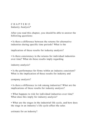
  • 27. such as retailing. Third, because goods must first be delivered to the stores, regulations that affect the cost of shipping by airplane, ship, or truck will affect retailers’ costs. Finally, lower tariffs and quotas will allow retailers to offer imported goods at lower prices (e.g., Walmart), which will expand their international production (outsourcing). 4 Technology can change natural monopolies. We mentioned earlier how some firms are generating their own electri- cal power. Another example is that, currently, numerous states are allowing electric utilities to compete for customers. Chapter 13: Industry Analysis 421 13.4 EVALUATING THE INDUSTRY LIFE CYCLE An insightful analysis when predicting industry sales and trends in profitability is to view the industry over time and divide its development into stages similar to those that humans prog- ress through: birth, adolescence, adulthood, middle age, old age. The number of stages in this industry life cycle analysis can vary based on how much detail you want. A five-stage model would include: 1. Pioneering development 2. Rapid accelerating growth 3. Mature growth 4. Stabilization and market maturity 5. Deceleration of growth and decline
  • 28. Exhibit 13.4 shows the growth path of sales during each stage. The vertical scale in logs reflects rates of growth, whereas the arithmetic horizontal scale has different widths representing dif- ferent, unequal time periods. To estimate industry sales, you must predict the length of time for each stage. This requires answers to such questions as: How long will an industry grow at an accelerating rate (Stage 2)? How long will it be in a mature growth phase (Stage 3) before its sales growth stabilizes (Stage 4) and then declines (Stage 5)? Besides being useful when estimating sales, this industry life cycle analysis also provides insights into profit margins and earnings growth, although these profit measures may not parallel the sales growth. The profit margin series typically peaks very early in the total cycle and then levels off and declines as competition is attracted by the early success of the industry. Exhibit 13.4 Life Cycle of an Industry Stage 1 Pioneering Development Stage 2 Rapid Accelerating
  • 29. Growth Stage 3 Mature Growth Stage 4 Stabilization and Market Maturity Stage 5 Deceleration of Growth and Decline Time Net Sales Log Scale 32 16 8 4
  • 30. 2 0 422 Part 4: Analysis and Management of Common Stocks The following is a brief description of how these stages affect sales growth and profits: 1. Pioneering development. During this start-up stage, the industry experiences modest sales growth and very small or negative profits. The market for the industry’s product or service during this stage is small, and the firms incur major development costs. 2. Rapid accelerating growth. During this rapid growth stage, a market develops for the prod- uct or service and demand becomes substantial. The limited number of firms in the indus- try face little competition, and firms can experience substantial backlogs and very high profit margins. The industry builds its productive capacity as sales grow at an increasing rate and the industry attempts to meet excess demand. High sales growth and high profit margins that increase as firms become more efficient cause industry and firm profits to explode (i.e., profits can grow at over 100 percent a year because of the low earnings base and the rapid growth of sales and margins). 3. Mature growth. The success in Stage 2 has satisfied most of
  • 31. the demand for the industry goods or service. Thus, future sales growth may be above normal, but it no longer acceler- ates. For example, if the overall economy is growing at 8 percent, sales for this industry might grow at an above normal rate of 15 percent to 20 percent a year. Also, the rapid growth of sales and the high profit margins attract competitors to the industry, causing an increase in supply and lower prices, which means that the profit margins begin to de- cline to normal levels. 4. Stabilization and market maturity. During this stage, which is probably the longest phase, the industry growth rate declines to the growth rate of the aggregate economy or its indus- try segment. During this stage, investors can estimate growth easily because sales correlate highly with an economic series. Although sales grow in line with the economy, profit growth varies by industry because the competitive structure varies by industry, and by individual firms within the industry because the ability to control costs differs among companies. Competition produces tight profit margins, and the rates of return on capital (e.g., return on assets, return on equity) eventually become equal to or slightly below the competitive level. 5. Deceleration of growth and decline. At this stage of maturity, the industry’s sales growth declines because of shifts in demand or growth of substitutes. Profit margins continue to be squeezed, and some firms experience low profits or even
  • 32. losses. Firms that remain prof- itable may show very low rates of return on capital. Finally, investors begin thinking about alternative uses for the capital tied up in this industry. Although these are general descriptions of the alternative life cycle stages, they should help you identify the stage your industry is in, which in turn should help you estimate its potential sales growth and profit margin. Obviously, everyone is looking for an industry in the early phases of Stage 2 and hopes to avoid industries in Stage 4 or Stage 5. Comparing the sales and earnings growth of an industry to similar growth in the economy should help you identify the indus- try’s stage within the industrial life cycle. 13.5 ANALYSIS OF INDUSTRY COMPETITION Similar to the sales forecast that can be enhanced by the analysis of the industrial life cycle, an industry earnings forecast should be preceded by the analyses of the competitive structure for the industry. Specifically, a critical factor affecting the profit potential of an industry is the in- tensity of competition in the industry, as Porter (1980a, 1980b, 1985) has discussed. 13.5.1 Competition and Expected Industry Returns Porter’s concept of competitive strategy is described as the search by a firm for a favorable competitive position in an industry. To create a profitable competitive strategy, a firm must Chapter 13: Industry Analysis 423
  • 33. first examine the basic competitive structure of its industry because the potential profitability of a firm is heavily influenced by the profitability of its industry. After determining the com- petitive structure of the industry, you examine the factors that determine the relative competi- tive position of a firm within its industry. In this section, we consider the competitive forces that determine the competitive structure of the industry. In the next chapter, our discussion of company analysis considers the factors that determine the relative competitive position of a firm within its industry. Basic Competitive Forces Porter believes that the competitive environment of an industry (the intensity of competition among the firms in that industry) determines the ability of the firms to sustain above-average rates of return on invested capital. As shown in Exhibit 13.5, he suggests that five competitive forces determine the intensity of competition and that the rel- ative effect of each of these five factors can vary dramatically among industries. 1. Rivalry among the existing competitors. For each industry analyzed, you must judge if the rivalry among firms is currently intense and growing, or polite and stable. Rivalry increases when many firms of relatively equal size compete in an industry. When estimating the num- ber and size of firms, be sure to include foreign competitors. Further, slow growth causes competitors to fight for market share and increases competition. High fixed costs stimulate
  • 34. the desire to sell at the full capacity, which can lead to price cutting and greater competition. Finally, look for exit barriers, such as specialized facilities or labor agreements. These can keep firms in the industry despite below-average or negative rates of return. Beyond these general conditions that impact competition, the following four factors will likewise affect the competitive environment within an industry: Exhibit 13.5 Forces Driving Industry Competition Potential Entrants Industry Competitors Rivalry among Existing Firms Suppliers Buyers Substitutes Threat of Substitute Products or Services Bargaining Power of BuyersBargaining Power of Suppliers Threat of New Entrants Source: Reprinted with the permission of The Free Press, an
  • 35. imprint of Simon & Schuster, Inc., from Competitive Strategy: Techniques for Analyzing Industries and Competitors by Michael E. Porter. Copyright © 1980, 1998 by The Free Press. All rights reserved. 424 Part 4: Analysis and Management of Common Stocks 2. Threat of new entrants. Although an industry may have few competitors, you must deter- mine the likelihood of firms entering the industry and increasing competition. High bar- riers to entry, such as low current prices relative to costs, keep the threat of new entrants low. Other barriers to entry include the need to invest large financial resources to compete as well as the availability of capital. Also, substantial economies of scale give a current in- dustry member an advantage over a new firm. Further, entrants might be discouraged if success in the industry requires extensive distribution channels that are hard to build be- cause of exclusive distribution contracts. Similarly, high costs of switching products or brands, such as those required to change a computer or telephone system, keep competi- tion low. Finally, government policy can restrict entry by imposing licensing requirements or limiting access to materials (lumber, coal). Without some of these barriers, it might be very easy for competitors to enter an industry, increasing the competition and driving down potential profit margins and rates of return.
  • 36. 3. Threat of substitute products. Substitute products limit the profit potential of an industry because they limit the prices firms in an industry can charge. Although almost everything has a substitute, you must determine how close the substitute is in price and function to the product in your industry. As an example, the threat of substitute glass containers hurt the metal container industry. Glass containers kept declining in price, forcing metal con- tainer prices and profits down. In the food industry, consumers constantly substitute be- tween beef, pork, chicken, and fish. The more commodity-like the product, the greater the competition and the lower the profit margins. 4. Bargaining power of buyers. Buyers can influence the profitability of an industry because they can bid down prices or demand higher quality or more services by showing a pro- pensity to switch among competitors. Buyers become powerful when they purchase a large volume relative to the sales of a supplier (e.g., Walmart, Home Depot). The most vulnera- ble firm is a one-customer firm that supplies a single large manufacturer, as is common for auto parts manufacturers or software developers. Buyers will be more conscious of the costs of items that represent a significant percentage of the firm’s total costs. This con- sciousness increases if the buying firm is feeling cost pressure from its customers. Also, buyers who know a lot about the costs of supplying an industry will bargain more intensely—for example, when the buying firm supplies some of
  • 37. its own needs and buys from the outside. 5. Bargaining power of suppliers. Suppliers can alter future industry returns if they increase prices or reduce the quality of the product or the services they provide. The suppliers are more powerful if there are few of them and if they are more concentrated than the indus- try to which they sell. Their power increases if they supply critical inputs to several indus- tries for which few, if any, substitutes exist. In this instance, the suppliers are free to change prices and services they supply to the firms in an industry. When analyzing sup- plier bargaining power, be sure to consider labor’s power within each industry. An investor needs to analyze these competitive forces to determine the intensity of the competition in an industry and assess the effect of this competition on the industry’s long- run profit potential. You should examine each of these factors and develop a relative competi- tive profile for each industry. It is important to consistently update this analysis of an indus- try’s competitive environment over time because an industry’s competitive structure can and will change over time. 13.6 ESTIMATING INDUSTRY RATES OF RETURN At this point, we have determined that industry analysis helps an investor select profitable in- vestment opportunities, and we have completed a thorough macroanalysis of the industry. Our next question is: How do we go about valuing an industry?
  • 38. Again, we consider the two equity Chapter 13: Industry Analysis 425 valuation approaches introduced in Chapter 11—the present value of cash flows and the rela- tive valuation ratios. Although our investment decision is always the same, the form of the comparison depends on which valuation approach is being used. In the case of the present value of cash flow tech- niques, we compare the present value of the specified cash flow and the prevailing value of the index and determine if we should underweight, equal weight, or overweight this global indus- try in our portfolio. When we value the industry using the alternative valuation ratios, an important addition to the analysis is that we also need to compare our industry ratios to the market ratios presented in Chapter 12. To demonstrate industry analysis, we use Standard and Poor’s retailing index to represent industry-wide data. This retailing index (hereinafter referred to as the RET industry) contains about 30 individual companies from several retailing sectors including two drugstores. There- fore, it should be reasonably familiar to most observers, and it is consistent with the subse- quent company analysis of Walgreens.
  • 39. 13.6.1 Valuation Using the Reduced Form DDM Recall that the reduced form DDM is: 13.1 Pi = D1 k − g where: Pi = the price of Industry i at Time t D1 = expected dividend for Industry i in Period 1 equal to D0ð1 þ gÞ k = the required rate of return on the equity for Industry i g = the expected long-run growth rate of earnings and dividend for Industry i As always, the two major estimates for any valuation model are k and g. We will discuss each of these at this point and also use these estimates subsequently when applying the two-step price/earnings ratio technique for valuation. Estimating the Required Rate of Return (k) Because the required rate of return (k) on all investments is influenced by the risk-free rate and the expected inflation rate, the differentiat- ing factor in this case is the risk premium for the retailing industry versus the market. In turn, we discussed the risk premium in terms of fundamental factors, including business risk (BR), financial risk (FR), liquidity risk (LR), exchange rate risk (ERR), and country (political) risk (CR). Alternatively, you can estimate the risk premium based on the CAPM, which implies
  • 40. that the risk premium is a function of the systematic risk (beta) of the asset. Therefore, to de- rive an estimate of the industry’s risk premium, you should examine the BR, FR, LR, ERR, and CR for the industry and compare these industry risk factors to those of the aggregate market. Alternatively, you can compute the systematic risk (beta) for the industry and compare this to the market beta of 1.0. Prior to calculating an industry beta, we briefly discuss the industry’s fundamental risk factors. Business risk is a function of relative sales volatility and operating leverage. As we will see when we examine the sales and earnings for the industry, the annual percentage changes in retailing sales were less volatile than aggregate sales as represented by PCE. Also, the OPM (operating profit margin) for retail stores was less volatile than for the S&P Industrials Index. Therefore, because both the sales and the OPM for the retailing industry have been less volatile than the market, operating profits are substantially less volatile. This implies that the business risk for the retailing industry is below average. 426 Part 4: Analysis and Management of Common Stocks The financial risk for this industry is difficult to judge because of widespread use of operat- ing leases for stores in the industry that are not included on the balance sheet. As a result, the reported data on debt to total capital or interest coverage ratios indicate that the FR for this
  • 41. industry is substantially below the market. Assuming substantial use of long-term lease con- tracts, when these are capitalized the retailing industry probably has financial risk about equal to the market. While data are not available to capitalize leases for the industry, we showed how to do this in Chapter 10 and will demonstrate it for a company in Chapter 14. To evaluate an industry’s market liquidity risk, you must estimate the liquidity risk for all the firms in the industry, and derive a composite view. The fact is, there is substantial varia- tion in market liquidity among the firms in this industry, ranging from Walgreens and Walmart, which are fairly liquid to small specialty retail chains, which are relatively illiquid. A conservative view is that the industry has above-average liquidity risk. Exchange rate risk (ERR) is the uncertainty of earnings due to changes in exchange rates faced by firms in this industry that sell outside the United States. The amount of ERR is determined by what proportion of sales is non-U.S., how these sales are distributed among countries, and the exchange rate volatility for these countries. This risk could range from an industry with very limited international sales (e.g., a service industry that is not involved overseas) to a global industry (e.g., the chemical or pharmaceutical industry). For a truly global industry, you need to examine the distribution of sales among specific countries because the exchange rate risk varies among countries based on the volatility of exchange rates with the
  • 42. U.S. dollar. The ERR for the retailing industry would be relatively low because sales and earnings for most retailing firms are attributable to activity within the United States. The existence of country risk (CR) is likewise a function of the proportion of foreign sales, the specific foreign countries involved, and the stability of the political/economic system in these countries. As noted, there is very little CR in the United Kingdom and Japan, but there can be substantial CR in China, Russia, and South Africa. Again, for the retailing industry, country risk would be relatively low because of limited foreign sales. In summary, for the retailing industry business risk is definitely below average, financial risk is at best equal to the market, liquidity risk is above average, and exchange rate risk and country risk are fairly low for most retail firms. The consensus is that the fundamental risk for the RET industry should be slightly lower than for the aggregate market. The systematic risk for the retailing industry is computed using the market model as follows: 13.2 % Δ RETt = αi + βið% Δ S&P 500tÞ where: % Δ RETt = the percentage price change in the retailing ðRETÞ index during month t αi = the regression intercept for the RET industry
  • 43. βi = the systematic risk measure for the RET industry equal to Covi;m=σ 2 m To derive an estimate for the RET industry, the model specified was run with monthly data for the five-year period of 2006 to 2010. The results for this regression are as follows: αi = 0:008 R 2 = 0:69 βi = 1:10 DW = 1:86 t-value = 5:45 F = 68:50 The systematic risk (β = 1.10) for the RET industry is a little above unity, indicating an above market risk industry (i.e., risk slightly above the market). These results suggest that the system- atic risk for this industry is a little above the prior estimate of fundamental risk factors (BR, FR, LR, ERR, CR). Chapter 13: Industry Analysis 427 Translating this systematic risk into a required rate of return estimate (k) calls for using the security market line model as follows: 13.3 ki = RFR + βiðRm − RFRÞ Recall that in Chapter 12 we derived three estimates for the
  • 44. required market rate of return based on alternative risk premiums (0.048 − 0.085 − 0.108). For our purposes here, it seems that the midpoint is reasonable—that is, a nominal RFR of 0.032 and an Rm of 0.072. This, combined with a beta for the industry at 1.10, indicates the following: k = 0:032 + 1:10ð0:04Þ = 0:032 + 0:044 = 0:076 = 7:60% For ease of computation, we will use a k of 8.0%. The fundamental risk analysis indicates risk slightly below the market and the CAPM estimate implies risk slightly above average. We pre- fer the 8 percent estimate for k in an environment of historically low Treasury rates. Estimating the Expected Growth Rate (g) Recall that earnings and dividend growth are determined by the retention rate and the return on equity: g = f (Retention Rate and Return on Equity) Again, we employ the three components of ROE: Net Profit Equity = Net Income
  • 45. Sales × Sales Total Assets × Total Assets Equity = Profit Margin × Total Asset Turnover × Financial Leverage We examine each of these variables in Exhibit 13.6 to determine if they imply a different ex- pected growth rate for RET versus the aggregate market (S&P Industrials Index). Earnings Retention Rate The data in Exhibit 13.6 indicate that the RET industry has a higher retention rate than the market (78 percent versus 63 percent), which implies a potentially higher growth rate, all else being the same (i.e., equal ROE).
  • 46. Return on Equity Because the return on equity is a function of the net profit margin, total asset turnover, and financial leverage, these three variables are examined individually. Historically, the data in Exhibit 13.6 show that the net profit margin for the S&P Industrials Index series has been consistently higher than the margin for the RET industry. This is not surprising because retail firms typically have lower profit margins but higher asset turnover. As expected, the total asset turnover (TAT) for the RET industry was higher than the average industrial company. In Exhibit 13.6, the average TAT for the S&P Industrials Index was 0.86 ver- sus 1.74 for the RET industry. Beyond the overall difference, as shown in Exhibits 13.6 and 13.7, the spread between the two series increased over the period because the industrials TAT experi- enced an overall decline, while the TAT for the RET industry experienced an overall increase. Multiplying the PM by the TAT indicates the industry’s return on total assets (ROTA). 5 Net Income Sales × Sales Total Assets =
  • 47. Net Income Total Assets The results in Exhibit 13.6 indicate that the return on total assets (ROTA) for the S&P In- dustrials Index series went from 3.27 percent in 1993 to 5.12 percent in 2009 and averaged 5 The reader is encouraged to read Appendix 13B to this chapter, which contains a discussion of an article by Selling and Stickney (1989), wherein they analyze the components of ROA and relate this to an industry’s economics and its strategy. 428 Part 4: Analysis and Management of Common Stocks E x h i b i t 1 3 . 6 E a r
  • 90. ’ H a n d b o o k . Chapter 13: Industry Analysis 429 4.72 percent, whereas the ROTA for the RET industry went from 4.07 percent to 5.73 percent and averaged 6.02 percent. Clearly, the industry ROTA results were superior on average to S&P Industrial results. The final component is the financial leverage multiplier (total assets/equity). As shown in Exhibits 13.6 and 13.8 both leverage multipliers experienced declines over the 17-year period— Exhibit 13.7 Time-Series Plot of Total Asset Turnover for the S&P Industrials and Retailing: 1993–2009 0.00 0.50
  • 91. 1.00 1.50 2.00 2.50 0.00 0.50 1.00 1.50 2.00 2.50 1993 1995 1997 1999 2001 2003 2005 2007 2009 Years A s s e ts /E q u
  • 92. it y ( F in a n c ia l L e v e ra g e ) RetailIndustrials Source: Standard and Poor’s Analysts’ Handbook. Exhibit 13.8 Time-Series Plot of Financial Leverage for the S&P Industrials and Retailing: 1993–2009
  • 94. 3.60 3.80 1993 1995 1997 1999 2001 2003 2005 2007 2009 Years A ss e ts /E q u it y ( F in a n ci a l L e
  • 95. v e ra g e ) Retai lIndustri al s Source: Standard and Poor’s Analysts’ Handbook. 430 Part 4: Analysis and Management of Common Stocks the industrials by 27 percent and the RET industry by 30 percent. Although the higher financial leverage multiplier implies greater financial risk for the S&P Industrials Index series, recall that the financial leverage for the RET industry is understated because the widely used leases are not capitalized. This final value of ROE in Exhibits 13.6 and 13.9 indicate that the best annual ROE varied by year until the last seven years when the RET industry was higher, except for 2008 when its profit margin experienced a large decline. The average annual ROEs were quite close—15.31 percent for the industrials, 15.76 percent for the RET industry. These average percentages are quite consistent with what would be derived from multiplying the averages of the components
  • 96. from Exhibit 13.6 as follows: ROE ESTIMATE BASED ON TOTAL PERIOD AVERAGES (1993–2009) Profit Margin Total Asset Turnover Total Assets/ Equity ROE S&P Industrials Index 5.93 × 0.86 × 3.03 = 15.45 RET Industry 3.57 × 1.74 × 2.61 = 16.21 Although examining the long-term historical trends and the averages for each of the com- ponents is important, you should not forget that expectations of future performance will deter- mine the ROE value for the industry, and these expectations probably will be heavily influenced by the recent years. To get more information regarding recent performance, it is in- sightful to examine the results for the recent five-year period (2005–2009) as follows: ROE ESTIMATE BASED ON RECENT FIVE-YEAR AVERAGES (2005–2009) Profit
  • 97. Margin Total Asset Turnover Total Assets/ Equity ROE S&P Industrials Index 6.17 × 0.86 × 2.75 = 14.59 RET Industry 4.08 × 1.68 × 2.33 = 15.97 Exhibit 13.9 Time-Series Plot of Return on Equity for the S&P Industrials and Retailing: 2005–2009 5.00 7.50 10.00 12.50 15.00 17.50 20.00 5.00
  • 98. 7.50 10.00 12.50 15.00 17.50 20.00 1993 1995 1997 1999 2001 2003 2005 2007 2009 Years R e tu rn o n E q u it y Industri al s Retai l Source: Standard and Poor’s Analysts’ Handbook.
  • 99. Chapter 13: Industry Analysis 431 Notably, using the recent results, the ROE results for the RET industry are still superior to the industrials with a slightly larger margin. Combining these recent ROE results with alternative retention rates provides the following growth estimates: GROWTH ESTIMATES BASED ON RECENT ROE WITH HISTORICAL AND RECENT RETENTION RATES Recent* ROE Hist.** RR Est. g Recent* ROE Recent* RR
  • 100. Est. g S&P Industrials Index 14.59 0.63 9.19 14.59 0.62 9.05 RET Industry 15.97 0.78 12.46 15.97 0.76 12.14 *Recent five-year average. **Total period average. Given the decrease in g for the industry when we consider the recent results, it is probably appropriate to use a growth estimate for the RET industry that is below the long-run historical estimate—that is, we will assume a near-term growth rate of 11 percent. Combining the Estimates At this point, we have the following estimates: k = 0:080 g = 0:11 D0 = $6:28 ðEstimated 2010 DividendsÞ D1 = $6:28 × 1:11= $6:97 ðEstimated Dividend for 2011Þ Because of the inequality between k and g (this g is above k and above the long-run market norm of about 7 percent and probably cannot be sustained), we need to evaluate this industry using the temporary growth company model discussed in Chapter 12. We will assume the fol- lowing growth pattern:
  • 101. 2011–2013 0.11 2014–2016 0.09 2017–2019 0.07 2020–onward 0.06 Using these estimates of k and this growth pattern, the computation of value for the industry using the DDM is contained in Exhibit 13.10. Exhibit 13.10 Dividend Discount Calculations Year Estimated Dividend Discount Factor @ 8% Present Value of Dividends 2011 6.97 — — 2012 7.74 0.9259 7.17 2013 8.59 0.8573 7.36 2014 9.36 0.7938 7.43 2015 10.20 0.7350 7.50 2016 11.12 0.6806 7.57 2017 11.90 0.6302 7.50 2018 12.73 0.5835 7.43 2019 13.62 0.5402 7.36 Continuing Valuea 722.00 0.5402 390.02
  • 102. Total Value $449.34 a Constant Growth Rate = 7% Continuing Value: D1 k − g = 13:62(1:06) 0:08−0:06 = 14:44 0:02 =722 432 Part 4: Analysis and Management of Common Stocks These computations imply a value of $449.34, compared to the stock price for the industry index of about $430 in early 2011. Therefore, according to this valuation model and these k and g estimates, this industry is currently about 4 percent undervalued. As will be shown, a fairly small change in the k − g spread can have a large effect on the estimated value. If we assumed a constant growth rate of 6 percent from the beginning and a D1 of $6.97, the value would be as follows:
  • 103. P = 6:97 ð0:08 − 0:06Þ = 6:97 0:02 = $348:50 Notably, this valuation likewise implies the industry is overvalued, even though it is a low esti- mate of value since it assumes the base growth rate of 6 percent from the beginning. The point is, the industry is undervalued assuming strong growth in the next few years, but also overva- lued assuming basic economic growth. Clearly, both valuations are dependent on the growth estimate. 13.6.2 Industry Valuation Using the Free Cash Flow to Equity (FCFE) Model We initially define the FCFE series and present the series for the recent 17-year period, along with an estimate for 2010 in Exhibit 13.11. Given these data, we consider the historical growth rates for the components and for the final FCFE series as inputs to estimating future growth for the valuation models. You will recall that FCFE is defined (measured) as follows: Net Income + Depreciation expense − Capital expenditures
  • 104. − Change in working capital − Principal debt repayments + New debt issues As noted, the FCFE data inputs and final annual value of FCFE for the RET industry for the period 1993–2010 is contained in Exhibit 13.11, along with 5- year and 10-year growth rates of the components. Using this data, we derive an estimate using the FCFE model under two scenar- ios: (1) a constant growth rate from the present, and (2) a two- stage growth rate assumption. The Constant Growth Rate FCFE Model We know that the constant growth rate model requires that the growth rate (g) be lower than the required rate of return (k), which we have specified as 8.00 percent. In the current case, this is difficult because the 10-year growth rate exceeds this. Still, in order to use the model, we assume a 10 percent growth in 2011 and 6 percent long-run growth in subsequent years. The result is as follows: g = 0:06 ðLong-Run Growth Beginning in 2012Þ k = 0:080 FCFE ð2010Þ = $21:83 FCFE ð2011Þ = $21:83ð1:10Þ = $24:01 = FCFE0 V = FCFE1 k − g
  • 105. = 24:01 ð1:06Þ 0:080 − 0:060 = 24:01 0:02 = $1,200 Chapter 13: Industry Analysis 433 This $1,200 value exceeds the industry stock price of $430 that prevailed in early 2011. This implies that the industry is substantially undervalued and should be overweighted in the portfolio. Notably, even if we assumed the long-run growth rate was only 5 percent, the estimated value would be $800, which would still imply that the industry is undervalued. The Two-Stage Growth FCFE Model As before, we assume a period of above-average growth for several years followed by a second period of constant growth at 6 percent. The period of above-average growth will be as follows based on an estimated initial 9 percent growth rate of FCFE, which is lower than what was used for dividends because the FCFE series has been fairly erratic over the past 17 years, including several years when the FCFE was negative.
  • 106. 2011 9% 2012 9% 2013 8% 2014 8% 2015 7% 2016 7% 2017–onward 6% If we assume a k of 8.0 percent and an FCFE of $21.83 in 2010, $23.79 in 2011, and $25.93 in 2012, the value for the industry is as shown in Exhibit 13.12. These results are very encourag- ing for the industry because the computed value of $1,368 is substantially above the recent market price of about $430. This apparent undervaluation would indicate that the industry should be overweighted in the portfolio. Exhibit 13.11 Components of Free Cash Flow to Equityholders for the Retail Industry Year Net Income Depreciation Expense Capital
  • 107. Expenditures Working Capital Change in Working Capital Principal Repayment Debt Issuance Total FCFE 1993 5.55 2.76 7.37 23.18 N/A N/A N/A N/A 1994 5.92 3.05 8.51 25.52 2.34 2.11 0.23 1995 5.26 3.77 8.93 30.50 4.98 7.41 2.53 1996 6.43 4.27 8.28 29.54 −0.96 0.36 3.74 1997 7.29 4.80 9.06 29.99 0.45 1.17 3.75 1998 9.66 5.24 10.51 28.02 −1.97 1.64 4.72 1999 10.65 6.01 12.93 24.67 −3.35 3.26 10.34 2000 9.50 6.52 15.60 23.24 −1.43 2.73 4.58 2001 9.83 7.25 15.76 33.66 10.42 4.09 −5.01
  • 108. 2002 13.20 7.00 14.23 33.21 −0.45 3.53 9.95 2003 19.16 9.11 15.70 51.11 17.90 3.57 −1.76 2004 20.47 10.57 17.98 56.02 4.91 10.05 −1.90 2005 20.07 11.38 19.44 45.27 −10.75 2.21 24.97 2006 27.96 13.05 23.83 48.27 3.00 16.29 30.47 2007 26.94 14.46 26.99 48.13 −0.14 23.85 38.40 2008 14.03 15.99 22.17 45.43 −2.70 2.95 13.50 2009 20.65 16.30 13.22 56.83 11.40 13.25 −0.92 2010(e) 24.00 17.00 20.00 60.00 3.17 4.00 21.83 5-year Growth Rate* 0.58% 8.65% −6.40% 10-year Growth Rate 11.74% 15.00% −1.53% *Growth rates are meaningful for Net Income, Depreciation, and CapEx and do not include the estimates for 2010. Source: Adapted from the Standard and Poor’s Analysts’ Handbook. 434 Part 4: Analysis and Management of Common Stocks Notably, the alternative present value of cash flow models have generated the following intrinsic values:
  • 109. Model Computed Value Constant growth DDM $348 Two-stage growth DDM $449 Constant growth FCFE $1,200 Two-stage growth FCFE $1,368 While there is a wide range of computed intrinsic values, three of four of them indicated that this industry is undervalued given its recent market price of $430. 13.7 INDUSTRY ANALYSIS USING THE RELATIVE VALUATION APPROACH This section contains a discussion and demonstration of the relative valuation ratio techniques: (1) price/earnings ratios (P/E), (2) the price to book value ratios (P/BV), (3) price to cash flow ratios (P/CF), and (4) price to sales ratios (P/S). We begin with the detailed demonstration of the P/E ratio approach, which provides a specific intrinsic value that equals an estimate of future earnings per share and an industry multiple. The analysis of the other relative valuation ratios is also more meaningful because we can compare the industry valuation ratios to the market valuation ratios while considering what factors affect the specific valuation ratios. 13.7.1 The Earnings Multiple Technique
  • 110. Again, the earnings multiple technique involves (1) a detailed estimation of future earnings per share, and (2) an estimate of an appropriate earnings multiplier (P/E ratio) based on a consid- eration of P/E determinants derived from the DDM. Estimating Earnings per Share To estimate earnings per share, you must start by estimat- ing sales per share. We initially describe three techniques that provide help and insights for the sales estimate. Next, we derive an estimate of earnings per share, which implies a net profit margin for the industry. As in Chapter 12, we begin the EPS estimate by estimating the oper- ating profit margin and operating profits. Then we subtract estimates of interest expense and then apply a tax rate to arrive at an estimate of earnings per share. Exhibit 13.12 Computation of Retail Industry Equity Value Using the FCFE Model and Two-Stage Growth Year FCFE Discount Factor @ 0.080 Present Value 2012 25.93 0.9259 24.01 2013 28.00 0.8573 24.00 2014 30.24 0.7938 24.00 2015 32.36 0.7350 23.78
  • 111. 2016 34.62 0.6806 23.56 Continuing Value 1,835.00 0.6806 01,248.90 Total Present Value $1,368.25 Continuing Value: 34:62(1:06) 0:08−0:06 = 36:70 0:02 =1,835 Chapter 13: Industry Analysis 435 Forecasting Sales per Share Recall that the macroanalysis of the industry included the follow- ing: (1) how the industry is impacted by the business cycle, (2) what structural changes have occurred within the industry, and (3) where the industry is in its life cycle, Based on this, the an- alyst would have a strong start regarding an industry sales estimate. We consider two general es- timation techniques (time series and input-output analysis) and a primary technique that should be used for almost all industries (i.e., a specific analysis of the industry-economy relationship). Time-Series Analysis A simple time-series plot of the sales for an industry can be very infor-
  • 112. mative regarding the pattern and the rate of growth for industry sales. Analyzing this series with an overlay of business cycle periods (expansions and recessions) and notations regarding major events will provide further insights. Finally, for many industries, you can extrapolate the time series to derive an estimate of sales. For industries that have experienced consistent growth, this can be an important estimate, especially if it is a new industry that has not yet developed a history with the economy. If the sales growth has been at a constant rate, you should use a semi-log scale where the constant growth shows as a straight line. Input-Output Analysis Input-output analysis provides useful insights regarding the outlook for an industry by identifying an industry’s suppliers and customers. This will indicate (1) the future demand from customers, and (2) the ability of suppliers to provide the goods and services required by the industry. The goal is to determine the long-run sales outlook for the industry’s suppliers and its major customers. In the case of global industries, you must include worldwide suppliers and customers. Industry-Economy Relationships The most rigorous and useful analysis involves comparing sales for an industry with one or several economic series that are related to the goods and ser- vices produced by the industry. The specific question is: What economic variables influence the demand for this industry? You should think about numerous factors that impact industry sales, how these economic variables will impact demand, and how
  • 113. they might interact. The following example demonstrates this industry-economy technique for the retailing industry (RET). Demonstrating a Sales Forecast The RET industry includes retailers of basic necessities, in- cluding pharmaceuticals, medical supplies, and nonmedical products, such as food and cloth- ing. Therefore, we want a series that (1) reflects broad consumption expenditures, and (2) gives weight to food and clothing. The economic series we consider are personal consumption expenditures (PCE) and PCE food, clothing, and shoes. Exhibit 13.13 contains the aggregate and per-capita values for these two series. These time-series data indicate that personal consumption expenditures (PCE) have experi- enced reasonably steady growth of about 7.7 percent a year during this period, while PCE food, clothing, and shoes has grown at a slower rate of about 4.6 percent. As a result, food, clothing, and shoes as a percentage of all PCE has declined from 14.1 percent in 1993 to only 11.0 percent in 2009. Obviously, as an analyst, you would be encouraged because even though sales of food, clothing, and shoes have grown slower than overall PCE, retail sales have grown faster than both of them at about 14.5 percent. The scatterplot in Exhibit 13.14 indicates a strong linear relationship between retail sales per share and sales of food, clothing, and shoes. Although not shown, there also is a good relationship with PCE. Therefore, if you can accurately estimate changes in these economic
  • 114. series, you should be able to estimate sales for RET. As the industry being analyzed becomes more specialized, you need a more unique economic series that reflects the demand for the industry’s unique product. The selection of several appro- priate economic series demonstrates an analyst’s knowledge and innovation. Also, industry sales are often dependent on several components of the economy, and in such a case you should con- sider a multivariate model that would include two or more economic series. For example, if you are analyzing the tire industry, you would need to consider new- car production, new-truck pro- duction, and a series that would reflect the replacement tire demand for both cars and trucks. 436 Part 4: Analysis and Management of Common Stocks You also should consider per-capita personal consumption expenditures. Although aggregate PCE increases each year, there also is an increase in the aggregate population, so the increase in PCE per capita (the average PCE for each adult and child) will be less than for the aggregate series. For example, during 2007, aggregate PCE increased about 5.2 percent, but per-capita PCE Exhibit 13.13 S&P Retail Sales and Various Economic Series: 1993–2009 Per Capita Year
  • 115. Retail Sales ($/Share) Personal Consumption Expenditures ($ Bn) PCE Food, Clothing, and Shoes ($ Bn) PCE ($) PCE Food, Clothing, and Shoes ($) Food, Clothing, and Shoes as % of PCE 1993 173.89 4483.6 632.6 21904 2430.44 14.11 1994 197.21 4750.8 659.5 22466 2503.27 13.88 1995 208.15 4987.3 674.9 22803 2531.62 13.53 1996 232.82 5273.6 701.4 23325 2600.53 13.30 1997 251.33 5570.6 722.3 23899 2646.19 12.97 1998 276.12 5918.5 744.3 24861 2695.24 12.58 1999 302.62 6342.8 784.7 25923 2809.24 12.37 2000 329.76 6830.4 818.3 26939 2897.48 11.98
  • 116. 2001 352.27 7148.8 837.6 27385 2935.50 11.72 2002 355.62 7439.2 848.4 27841 2944.47 11.40 2003 383.89 7804.0 880.1 28357 3026.01 11.28 2004 444.61 8285.1 928.2 29072 3162.50 11.20 2005 476.54 8819.0 980.5 29771 3309.94 11.12 2006 580.68 9322.7 1028.1 30341 3437.86 11.03 2007 605.18 9806.3 1076.3 30757 3563.61 10.98 2008 598.70 10104.5 1109.3 30394 3639.07 10.98 2009 578.46 10001.3 1100.1 29770 3577.76 11.00 Compound Annual Growth Rate 14.54% 7.69% 4.62% 2.24% 2.95% −1.38% Source: Bureau of Economic Analysis. Exhibit 13.14 Scatterplot of Retail Sales per Share and PCE— Food, Clothing, and Shoes: 1993–2009 100 200 300 400
  • 117. 500 600 700 100 200 300 400 500 600 700 600 800 1000 1200 PCE—Food, Clothing, and Shoes ($ Bn) R e ta il S a le s
  • 118. p e r S h a re $ Chapter 13: Industry Analysis 437 increased only 1.0 percent. Finally, an analysis of the relationship between percent change in an economic variable and percent changes in industry sales will indicate how the two series move together and would be sensitive to any changes in the relationship. Using annual percentage changes provides the following regression model: 13.4 %Δ Industry Sales = αi + βi(%Δ in Economic Series) The size of the βi coefficient should indicate how closely the two series move together. Assum- ing the intercept (αi) is close to zero, a slope (βi) value of 1.00 would indicate relatively equal percent changes (e.g., a 10 percent increase in PCE typically is associated with a 10 percent increase in industry sales). A βi larger than unity would imply that industry sales are more volatile than the economy is. This analysis and the levels
  • 119. relationship reflected in Exhibit 13.14 would help you find an economic series that closely reflects the demand for the indus- try’s products; it also would indicate the form of the relationship. As indicated, there was a good relationship between retail sales and PCE—Food, Clothing, and Shoes. The specific regression relationship was: 13.5 % Δ Retail Sales = − 0:05 + 2:52ð%Δ PCE— Food, Clothing, and ShoesÞ r2 = 0:37 Given the regression results, the specific sales forecast begins with an estimate of aggregate PCE growth for the years in question (i.e., 2010 and 2011). Because of the importance of PCE as a component of the economy, several estimates of PCE are available. The next step is to estimate the proportion of PCE spent on food, clothing, and shoes that has declined from 14.11 percent to 11 percent. You apply an estimate of this proportion to the PCE estimate and derive an estimate of the percent change in PCE—Food, Clothing, and Shoes that is used in the retail store sales regression model. To demonstrate this process, we examined several economic sources that indicated that nominal PCE increased by 5.1 percent in 2010 (to $10,511 billion) and the projection was for an increase in 2011 of 6.3 percent to $11,173 billion. Regarding the percent of PCE spent on food, clothing, and shoes, we expect this proportion to increase slightly with the slow recovery
  • 120. of the economy—we estimate 11.02 percent in 2010 and 11.04 percent in 2011. This implies values for PCE—Food, Clothing, and Shoes of $1,158 billion in 2010 and $1,233 billion in 2011, which implies growth in this series of 5.3 percent in 2010 and 6.5 percent in 2011. Using these percentages in the Equation 13.5 regression provides an estimate of retail stores sales growth of 8.4 percent for 2010 ($627) and 11.38 percent for 2011 ($698). These sales growth rates are conservative relative to the long-run results in this industry (which was over 14 per- cent a year), but reflect the sluggish economic recovery in 2010 and 2011. Forecasting Earnings per Share After the sales forecast, it is necessary to estimate the in- dustry’s profitability based on an analysis of the industry income statement. An analyst should also benefit from the prior macroanalysis that considered where the industry is in its life cycle, which impacts its profitability. How does this industry relate to the business cycle, and what does this imply regarding profit margins at this point in the cycle? Most important, what did you conclude regarding the competitive environment in the industry, and what does this mean for the profitability of sales? Industry Profit Margin Forecast Similar to the aggregate market, the net profit margin is the most volatile and the hardest margin to estimate directly. Alternatively, it is suggested that you begin with the operating profit margin (EBIT/Sales) and then estimate interest expense and the tax rate.
  • 121. The Industry’s Operating Profit Margin Recall that in the market analysis, we analyzed the fac- tors that should influence the economy’s operating profit margin, including capacity utilization, 438 Part 4: Analysis and Management of Common Stocks unit labor cost, inflation, and net exports. The most important variables were capacity utilization and unit labor cost. We cannot do such an analysis for most industries because these variables (capacity utilization and unit labor cost) typically are not available for individual industries. As an alternative, we can assume that movements in these industry profit margin variables are re- lated to movements in similar economic variables. For example, if we assume an increase in ca- pacity utilization for the aggregate economies, there is probably a comparable increase in utilization for the auto industry or the chemical industry. The same could be true for unit labor cost. If there is a stable relationship between these variables for the industry and the economy, we would expect a relationship to exist between the profit margins for the industry and the economy. Although it is not necessary that the relationship be completely linear, it is important for the relationship (whatever it is) to be generally stable. The operating profit margin (OPM) for the S&P Industrials Index and the RET industry is presented in Exhibit 13.15. The time-series plot in Exhibit 13.16 indicates that the S&P Indus-
  • 122. trials Index OPM experienced a steady increase from 1993 through 2000, followed by a decline during the recession year 2001. The margins slowly recovered from 2002 through 2007, but had small declines during the recession in 2008–2009. The RET industry OPM likewise experi- enced a fairly steady increase that peaked in 1999, followed by small declines in 2000 and 2001, a recovery in 2002 to a peak in 2005, gradual declines through 2008, and a small recov- ery in 2009. The regression analysis of the relationship between the OPM for the market and industry was not useful, so it is not discussed. Apparently, the best estimate for the RET indus- try is the OPM time-series plot using what we know about the changing competitive environ- ment and profit trends in the retail business. The point is, any quantitative analysis should be a supplement to the macroanalysis of the competitive environment for the industry. Regression analysis and the time-series analysis are both useful tools, but neither technique should be applied mechanically. You should be aware of any unique factors affecting the indus- try, such as price wars, contract negotiations, building plans, or foreign competition. These unique events can significantly impact an estimate of the gross profit margin or a range of industry profit margins (optimistic, pessimistic, most likely). Beyond this estimation of the near-term OPM, it is important to consider the long-term profitability of the industry based on its competitive structure. Industry Interest Expense An industry’s interest expense will be
  • 123. a function of its financial leverage and interest rates. As shown in Exhibit 13.17, interest expense for the RET industry has always been relatively low and stable compared to the S&P Industrials Index. Because there is not a relationship between the two interest expense series, an analyst would need to derive his/ her own estimate based on two separate estimates: (1) changes in the amount of debt outstand- ing for this industry, and (2) the trend in interest rates (will they increase or decline?). Estimating Interest Expense The historical data needed to estimate interest expense are in Exhibit 13.17, and we can use the following steps: 1. Estimate the annual total asset turnover (TAT) for the RET industry. 2. Use your 2011 sales and TAT forecasts to estimate total assets. 3. Estimate the long-term (interest-bearing) debt as a percentage of total assets for the RET industry. 4. Based on your estimate of total assets and the percent of long-term debt to total assets, estimate the dollar value of long-term debt. 5. Estimate the annual interest cost as a percentage of long-term debt based upon prior esti- mates of market yields. 6. Estimate interest expense based on the following: (Estimated Interest Cost of Debt) × (Estimated Long-Term Debt)
  • 124. Chapter 13: Industry Analysis 439 E x h i b i t 1 3 . 1 5 P r o fi t M a r g in s a n d C
  • 161. n d b o o k . 440 Part 4: Analysis and Management of Common Stocks For example, our sales estimate of $698 and a TAT that has averaged about 1.63 over the recent years imply total assets of $428 next year. Long-term interest- bearing debt has averaged about 20 percent of total assets for the RET industry recently, so we will use that percent for 2011, which implies debt of $85.60 (0.20 × $428). In turn, interest expense as a percentage of long-term debt Exhibit 13.16 Time-Series Plot of the Operating Profit Margin for the S&P Industrials and Retail Industries: 1993–2009 4.00 6.00 8.00 10.00 12.00
  • 162. 14.00 16.00 18.00 4.00 6.00 8.00 10.00 12.00 14.00 16.00 18.00 1993 1995 1997 1999 2001 2003 2005 2007 2009 Years O p e ra ti n g
  • 163. P ro & t M a rg in % Industri al s Retai l Exhibit 13.17 Components for Deriving Specific Estimates for Interest Expense for the Retail Industry: 1993–2009 Year Sales Total Assets Total Asset Turnover LT Debt LT Debt as % of Total Assets Interest Expense Interest Exp. as % of LT Debt 1993 173.89 131.73 1.32 23.59 17.91 2.43 10.30
  • 164. 1994 197.21 136.95 1.44 25.01 18.26 1.90 7.60 1995 208.15 131.74 1.58 32.63 24.77 2.81 8.61 1996 232.82 127.22 1.83 32.62 25.64 3.01 9.23 1997 251.33 135.85 1.85 34.54 25.42 2.60 7.53 1998 276.12 140.88 1.96 34.65 24.60 2.99 8.63 1999 302.62 149.81 2.02 36.15 24.13 2.76 7.63 2000 329.76 163.25 2.02 36.99 22.66 3.09 8.35 2001 352.27 176.14 2.00 43.54 24.72 3.18 7.30 2002 355.62 189.16 1.88 44.96 23.77 2.72 6.05 2003 383.89 229.87 1.67 47.76 20.78 3.33 6.97 2004 444.61 267.84 1.66 41.13 15.36 2.72 6.61 2005 476.54 280.32 1.70 44.08 15.73 2.66 6.03 2006 580.68 317.31 1.83 59.17 18.65 3.26 5.51 2007 605.18 360.23 1.68 78.44 21.78 4.39 5.60 2008 598.70 369.57 1.62 79.06 21.39 4.60 5.82 2009 578.46 363.81 1.59 71.63 19.69 4.75 6.63 Means 1.74x 21.48% 7.32% Source: Standard and Poor’s Analysts’ Handbook.
  • 165. Chapter 13: Industry Analysis 441 (the industry’s approximate debt cost) during the recent period has been between 4 and 5 percent. Based on the declines in market interest rates during 2010 and early 2011, we would estimate a debt rate of 4.50 percent. This interest rate estimate combined with our long-term debt estimate of $85.60 implies interest expense of $3.85 (0.045 × $85.60). Industry Tax Rate As you might expect, tax rates differ between industries. An extreme exam- ple would be the oil industry, in which heavy depletion allowances cause lower taxes. Gener- ally, you can assume that tax law changes are consistent across industries. To see if this is valid, you need to examine the relationship of tax rates over time for your industry and the aggregate market to determine if you can use regression analysis in your estimation process. Alternatively, a time-series plot could provide a useful estimate. Exhibit 13.19 indicates that the RET industry tax rate has been between 31 and 35 percent and has been at or below the lower boundary in recent years. Therefore, we would use 32 per- cent, although you still need to consider pending national legislation and unique industry tax factors. Using this estimated tax rate, you multiply the EBT per share value by (1 − 0.32) to get your estimate of earnings per share (EPS). In addition to estimating EPS, you also should examine the industry’s net profit margin as a
  • 166. check on your EPS estimate. A time-series plot of the net profit margin series for the industry and the S&P Industrials Index is contained in Exhibit 13.20. Notably, both series experienced an overall increase of about 2 percent, but the RET industry has been less volatile. An Industry Earnings Estimate Example To help you understand the procedure, the follow- ing is an estimate of earnings per share for the RET industry. A practicing analyst would use this example as an initial estimate that would be modified based on his or her industry knowl- edge, current events, and expectations of unique factors. Given that the best relationship was between RET industry sales and PCE—Food, Clothing, and Shoes, we estimated PCE and PCE—Food, Clothing, and Shoes as a percent of PCE and derived a RET sales estimate of $698 per share. Exhibit 13.18 Time-Series Plot of Interest Expense for the Industrials and Retail Industry: 1993–2009 0.00 5.00 10.00 15.00 20.00
  • 167. 25.00 0.00 5.00 10.00 15.00 20.00 25.00 1993 1995 1997 1999 2001 2003 2005 2007 2009 Years In te re st E x p e n se $ /S
  • 168. h a re Industri al s Retai l 442 Part 4: Analysis and Management of Common Stocks As noted earlier, the OPM for the RET industry recovered from the recession in 2002 and experienced strong performance during 2003 through 2007. Following a decline during the 2008 recession, the margin recovered to almost 6 percent in 2009. We estimate a further re- covery to 6.50 percent in 2010 and 7.00 percent in 2011, which implies operating profits in 2011of $48.86 (0.07 × $698). Exhibit 13.19 Time-Series Plot of Effective Tax Rates for the Industrials and Retail Industry: 1993–2009 25.00 27.00 29.00 31.00 33.00
  • 170. e ct iv e T a x R a te s % Industri al s Retai l Source: Standard and Poor’s Analysts’ Handbook. Exhibit 13.20 Time-Series Plot of the Net Profit Margin for the Industrials and Retail Industry: 1993–2009 0.00 1.00 2.00 3.00
  • 172. P ro & t M a rg in % Industri al s Retai l Chapter 13: Industry Analysis 443 Given the declining yields during 2010 and the flat interest rates envisioned during 2011, our estimate of interest expense was $3.85 in 2011. Thus, EBT would be $45.01 (48.86 − 3.85). As noted earlier, the tax rate for the RET industry has consistently been in the 31–35 per- cent range in recent years, and 32 percent seems appropriate for 2011. This implies net income of $30.61 (45.01 × 0.68) and a net profit margin for the RET industry of 4.39 percent (30.61/ 698), which is similar to the 2007 margin. Given an estimate of the industry’s net income per share (for simplicity, we will round the EPS estimate to $31 per share), the next step is to estimate the
  • 173. earnings multiplier for this industry. Estimating an Industry Earnings Multiplier In this section, we discuss how to estimate an industry earnings multiplier using two alternative techniques: macroanalysis and microanal- ysis. In macroanalysis, you examine the relationship between the multiplier for the industry and the market. In microanalysis, you estimate the multiplier by examining the specific vari- ables that influence it: (1) the dividend-payout ratio, (2) the required rate of return for the in- dustry (k), and (3) the expected growth rate of earnings and dividends for the industry (g). Macroanalysis of an Industry Multiplier: Why a Relationship? This subsection considers the relationship between the earnings multiplier (P/E ratio) for an industry to the P/E for the ag- gregate market. We expect a relationship based on the variables that influence the multiplier— the required rate of return, the expected growth rate of earnings and dividends, and the divi- dend-payout ratio. Specifically, as discussed, the required rate of return (k) is a function of the nominal risk-free rate (which is the same for all investments) plus a risk premium, which is the major reason for differences in k. Also, while the risk premium may differ between the market and an industry, any changes in the risk premium for the market and the industry are probably related. Clearly, the rate of growth (g) for an industry may differ from that of the market and is a